Credal Bayesian Deep Learning
Abstract.
Uncertainty quantification and robustness to distribution shifts are important goals in machine learning and artificial intelligence. Although Bayesian Neural Networks (BNNs) allow for uncertainty in the predictions to be assessed, different sources of predictive uncertainty cannot be distinguished properly. We present Credal Bayesian Deep Learning (CBDL). Heuristically, CBDL allows to train an (uncountably) infinite ensemble of BNNs, using only finitely many elements. This is possible thanks to prior and likelihood finitely generated credal sets (FGCSs), a concept from the imprecise probability literature. Intuitively, convex combinations of a finite collection of prior-likelihood pairs are able to represent infinitely many such pairs. After training, CBDL outputs a set of posteriors on the parameters of the neural network. At inference time, such posterior set is used to derive a set of predictive distributions that is in turn utilized to distinguish between (predictive) aleatoric and epistemic uncertainties, and to quantify them. The predictive set also produces either (i) a collection of outputs enjoying desirable probabilistic guarantees, or (ii) the single output that is deemed the best, that is, the one having the highest predictive lower probability – another imprecise-probabilistic concept. CBDL is more robust than single BNNs to prior and likelihood misspecification, and to distribution shift. We show that CBDL is better at quantifying and disentangling different types of (predictive) uncertainties than single BNNs and ensemble of BNNs. In addition, we apply CBDL to two case studies to demonstrate its downstream tasks capabilities: one, for motion prediction in autonomous driving scenarios, and two, to model blood glucose and insulin dynamics for artificial pancreas control. We show that CBDL performs better when compared to an ensemble of BNNs baseline.
Key words and phrases:
Bayesian deep learning; imprecise probabilities; credal sets; epistemic and aleatory uncertainties; uncertainty quantification; machine learning robustness2010 Mathematics Subject Classification
Primary: 68T37; Secondary: 68T05, 68W251. Introduction
One of the greatest virtues an individual can have is arguably being aware of their own ignorance, and acting cautiously as a consequence. Similarly, an autonomous system using neural networks (NNs) would greatly benefit from understanding the probabilistic properties of the NN’s output (for example, its robustness to distribution shift), in order to incorporate them into any further decision-making. This paper collocates on the path of giving a machine such a desirable quality.
In the last few years, there has been a proliferation of work on calibrating (classification) NNs, in order to estimate the confidence in their outputs [54] or to produce conformal sets that are guaranteed to contain the true label, in a probably approximately correct (PAC) sense [95]. While such methods are a promising first step, they require a calibration set (in addition to the original training set) and cannot be directly used on Out-Of-Distribution data without further examples.
Bayesian Neural Networks (BNNs) offer one approach to overcome the above limitations. The Bayesian paradigm provides a rigorous framework to analyze and train uncertainty-aware neural networks, and more generally to support the development of learning algorithms [64]. In addition, it overcomes some of the drawbacks of deep learning models, namely that they are prone to overfitting, which adversely affects their generalization capabilities, and that they tend to be overconfident about their predictions when they provide a confidence interval. BNNs, though, are trained using a single prior, which may still suffer from miscalibration and robustness issues [81].
In this work we introduce Credal Bayesian Deep Learning (CBDL), a procedure that draws on concepts from the imprecise probability (IP) literature [4, 109, 113]. Unlike other techniques in the fields of artificial intelligence (AI) and machine learning (ML) involving imprecise probabilities – that typically only focus on classification problems – CBDL can be used for both classification and regression. It captures the ambiguity the designer faces when selecting which prior to choose for the parameters of a neural network, and which likelihood distribution to choose for the training data at hand.
CBDL can be thought of as a NN trained using prior and likelihood finitely generated credal sets (FGCSs), and , respectively.11 1 Intuitively, the larger these credal sets, the higher prior and likelihood ambiguity the user faces. They are convex sets of probability measures having finitely many extreme elements (the elements that cannot be written as a convex combination of one another), and , respectively (see also Remark 2). A very simple example of a prior FGCS is the collection of all the convex combinations of two one-dimensional Normal distributions and , i.e.,
Consequently, in this toy example we have that . FGCSs are further examined in section 2.2.
Given the use of finitely generated credal sets, CBDL can also be seen as a non-condensed (uncountably) infinite ensemble of BNNs – each BNN corresponding to a pair of prior from the prior FGCS and likelihood from the likelihood FGCS . Such infinite ensemble, though, is carried out using only finitely many elements, that is, only pairs of components of the sets of extreme elements and . This because every element of can be obtained from a convex combinations of the elements of , and similarly for the likelihood FGCS. After training, CBDL produces a posterior FGCS on the parameters of the neural network. At inference time, is used to derive a predictive FGCS , that is, given a new input, a set of plausible distributions over the space of outputs.22 2 As we shall see in section 3.1, since computing the posteriors and the predictive distributions is oftentimes an intractable problem, we approximate the elements of and of using Variational Inference (VI). As a consequence, we denote the VI-approximated posterior and predictive credal sets as and , respectively. In turn, generates a set of outputs – or a single output, depending on the user’s needs – that enjoys desirable probabilistic guarantees, even when the elements of credal set are approximated, e.g. using variational inference. CBDL also gives a way of quantifying and disentangling different types of uncertainties within .
We use a credal set approach to overcome some of the drawbacks of single BNNs. In particular, CBDL allows to counter the criticism to the practice in (standard) Bayesian statistics of (i) using a single, arbitrary prior to represent the initial state of ignorance of the agent, (ii) using non-informative priors to model ignorance, and (iii) using a single, arbitrary likelihood to represent the agent’s knowledge about the sampling model.33 3 Criticisms (i) and (iii) are also pointed out in [85, Section 2.2]. As a consequence, credal sets make the analysis more robust to prior and likelihood misspecification. In addition, they make it possible to quantify and distinguish between epistemic and aleatoric uncertainties (EU and AU, respectively). This is desirable in light of several areas of recent ML research, such as Bayesian deep learning [39, 69], adversarial example detection [105], and data augmentation in Bayesian classification [67].
AU refers to the uncertainty that is inherent to the data generating process; as such, it is irreducible. Think, for example, of a coin toss. No matter how many times the coin is tossed, the stochastic variability of the experiment cannot be eliminated. EU, instead, refers to the lack of knowledge about the data generating process; as such, it is reducible. It can be lessened on the basis of additional data. For example, after only a few tosses, we are unable to gauge whether a coin is biased or not, but if we repeat the experiment long enough, this type of uncertainty vanishes. We note in passing that predictive EU cannot be adequately captured using a single BNN [59, 44]. One reason for this is that selecting a unique prior and a unique likelihood implicitly assumes perfect knowledge around the true prior and the true data generating process. Another, more subtle one, is explored in the last paragraph of section 2.1. Methods that disentangle between the two types of (predictive) uncertainties that are based on a single distribution are ad-hoc, but are not theoretically well-justified. EU can be typically reduced by retraining the model using an augmented training set [83] (e.g. via semantic preserving transformations [68], Puzzle Mix [70], etc.). On the other hand, since AU is irreducible, there is an increasing need for ML techniques that are able to detect and flag its excess, so that the user can “proceed with caution”.
Remark 1.
EU should not be confused with the concept of epistemic probability [35, 36, 113]. In the subjective probability literature, epistemic probability can be captured by a single distribution. Its best definition can be found in [113, Sections 1.3.2 and 2.11.2]. There, the author specifies how epistemic probabilities model logical or psychological degrees of partial belief of the agent. We remark, though, how de Finetti and Walley work with finitely additive probabilities, while in this paper we use countably additive probabilities.
The motivation for working with credal sets is threefold: (i) it allows to be robust against prior and likelihood misspecification; (ii) unlike when using a single probability distribution, it permits to represent ignorance in the sense of lack of knowledge; (iii) it allows to quantify and disentangle between EU and AU. A more in-depth discussion can be found in Appendix A. In addition, we point out that despite a hierarchical Bayesian model (HBM) approach seems to be a viable alternative to one based on credal sets, these latter are better justified philosophically, and do not suffer from the same theoretical shortcomings of HBM procedures [9, 59, 63, 113]. A more detailed explanation can be found in Appendix B. Let us mention that we only compare CBDL against Bayesian techniques because a comparison against non-Bayesian ones is either difficult to justify, or unfair. Indeed, the initial knowledge component, captured by the prior distribution (or the set of priors, in our case), has no direct comparisons with other approaches. Take conformal prediction [111, 103, 50, 6] for instance. It is a model-free method, which means that no prior knowledge around the experiment at hand is required. The only choice the user makes is which non-conformity score to use. How would we compare this approach with the choice of different priors, which conveys the idea that the user knows that a true distribution over the space of neural network parameters exists, but it is not fully known? In addition, despite the ubiquitous claim that conformal prediction (CP) is an uncertainty quantification tool, it is actually not. CP is an uncertainty representation tool. Indeed, CP represents uncertainty via the conformal prediction region (on the other hand, in this paper we represent uncertainty via credal sets). It does not quantify it: there is no real value attached to any kind of predictive uncertainty (aleatoric or epistemic). Some claim that the diameter of the conformal prediction region quantifies the uncertainty, but even in that case, it is unable to distinguish between AU and EU. Indeed, the diameter is a positive function of both: it increases as both increase, and hence it cannot be used to distinguish between the two.
We summarize our contributions next: (1) We present CBDL, and develop the theoretical tools and the algorithm required to use it in practice. (2) We show that a CBDL approach is more robust than single BNNs to prior and likelihood misspecification, and to distribution shifts. We also explain how, during inference, the credal set of posteriors on the network parameters obtained during training is used to derive a credal set of predictive distributions , and in turn a set of outcomes -- or a single outcome -- that enjoys probabilistic guarantees.44 4 Once again, as we shall see in section 3.1, we approximate the elements of the posterior and the predictive credal sets using Variational Inference (VI). (3) We show how CBDL is better at quantifying and disentangling predictive AU and EU than single BNNs and ensemble of BNNs.55 5 We note in passing how recently [91] show that (finite) deep ensembles are the current state-of-the-art methods for quantifying and disentangling different types of uncertainties on ImageNet. Our experiments show that CBDL improves on (finite) ensembles of BNNs, both in uncertainty quantification and disentanglement, and in downstream tasks performances. Together with the findings in [91], this is an additional argument in favor of the effectiveness of our methodology. We also apply CBDL to two safety critical systems to demonstrate its downstream tasks capabilities. One, motion prediction for autonomous driving, and two, the human insulin and blood glucose dynamics for artificial pancreas control. We demonstrate improvements in both these settings with respect to ensemble of BNNs methods, the reason being that better uncertainty quantification leads to a positive impact on the decisions made using them.
Before moving on, let us point out that while CBDL pays a computational price coming from the use of credal sets, it is able to quantify both (predictive) EU and AU, and to do so in a principled manner, unlike single and ensembles of BNNs. In addition, it requires less stringent assumptions on the nature of the prior and likelihood ambiguity faced by the agent than other imprecise-probabilities-based techniques, as explained in Appendices B and L. We also stress that if the user prioritizes computational efficiency, they should use non-Bayesian methods, as they are faster to implement than Bayesian techniques. In safety-critical situations instead – where using uncertainty-informed methods is crucial for quantifying the types of uncertainties, but also for the outcome of the analysis at hand – CBDL is a natural choice.
Structure of the Paper. Section 2 presents the needed preliminary concepts, followed by section 3 that introduces and discusses the CBDL algorithm, together with its theoretical properties. We present our experimental results in section 4, and we examine the related work in section 5. Section 6 concludes our work. In the appendices, we give further theoretical and philosophical arguments and we prove our claims.
Notation Summary. In this paper, we make extensive use of different notation and acronyms. We summarize them in Table 1 to help the reader navigate through them.
| Notation and Acronyms | Meaning | ||
|---|---|---|---|
| FGCS | Finitely Generated Credal Set | ||
| CBDL | Credal Bayesian Deep Learning | ||
| Upper case latin letters, such as and | Probability measures, e.g. prior or likelihood | ||
| Lower case latin letters, such as and | The pdf/pmf associated to probability measures | ||
| A finite collection of probability measures | |||
| The convex hull operator | |||
| |||
| A prior FGCS | |||
| A likelihood FGCS | |||
| A posterior FGCS | |||
| VI | Variational Inference | ||
| |||
| A predictive FGCS | |||
| |||
| The extreme elements of an FGCS | |||
| BNN | Bayesian Neural Network | ||
| |||
| EBNN | Ensemble of Bayesian Neural Networks | ||
| Function representing the neural network architecture | |||
| , | Lower and upper probabilities, respectively | ||
| HDR | Highest Density Region | ||
| IHDR | Imprecise Highest Density Region | ||
| |||
| Entropy of probability measure | |||
| , | Upper and lower entropy associated with a credal set | ||
| Epistemic Uncertainty encoded in an FGCS | |||
| Aleatoric Uncertainty encoded in an FGCS | |||
| Total Uncertainty encoded in an FGCS | |||
| Cardinality of a generic set | |||
| , |
| ||
| BMA | Bayesian Model Averaging |
2. Background and Preliminaries
In this section, we present the background notions that are needed to understand our main results. In section 2.1 we introduce Bayesian Neural Networks. Section 2.2 discusses (finitely generated) credal sets, upper and lower probabilities, and imprecise highest density regions. Section 2.3 introduces the concepts of upper and lower entropy, which are used to quantify and disentangle AU and EU. The reader familiar with these concepts can skip to section 3.
2.1. Bayesian Neural Networks
In line with the recent survey on BNNs by [64], Bayes’ theorem can be stated as , where is a hypothesis about which the agent holds some prior beliefs, and is the data the agent uses to update their initial opinion. Probability distribution represents how likely it is to observe data if hypothesis were to be true, and is called likelihood, while probability distribution represents the agent’s initial opinion around the plausibility of hypothesis , and is called prior. The evidence available is encoded in , while posterior probability represents the agent’s updated opinion. Using Bayes’ theorem to train a predictor can be understood as learning from data : the Bayesian paradigm offers an established way of quantifying uncertainty in deep learning models.
BNNs are stochastic artificial neural networks (ANNs) trained using a Bayesian approach [18, 52, 64, 78, 107, 114]. The goal of ANNs is to represent an arbitrary function . Let represent the parameters of the network, and call the space belongs to. Stochastic neural networks are a type of ANN built by introducing stochastic components to the network. This is achieved by giving the network either a stochastic activation or stochastic weights to simulate multiple possible models with their associated probability distribution. This can be summarized as , , where depends on to highlight the stochastic nature of the neural network, is the density of a probability measure on ,66 6 We can write as the Radon-Nikodym derivative of with respect to some -finite dominating measure , that is, . and represents random noise to account for the fact that function is just an approximation. The connection between the BNN notation and the general one of the Bayes’ theorem is explained in the next two paragraphs.
To design a BNN, the first step is to choose a deep neural network architecture, that is, functional model . Then, the agent specifies the stochastic model, that is, a prior distribution over the possible model parametrization , and a prior confidence in the predictive power of the model . Given the usual assumption that multiple data points from the training set are independent, the product represents the likelihood of outputs given inputs and parameter , where (a) is the training set; (b) is the collection of training inputs, which is a subset of the space of inputs; (c) is the collection of training outputs, which is a subset of the space of outputs.
The model parametrization can be considered to be hypothesis . Following [64], we assume independence between model parameters and training inputs , in formulas . Hence, Bayes’ theorem can be rewritten as
Notice that the equality comes from having assumed . Posterior density is typically high dimensional and highly nonconvex [62, 64], so computing it and sampling from it is a difficult task. The first issue is tackled using Variational Inference (VI) procedures, while Markov Chain Monte Carlo (MCMC) methods address the second challenge. Both are reviewed – in the context of machine learning – in [64, Section V], where the authors also inspect their limitations. BNNs can be used for both regression and classification [64, Section II]; besides having a solid theoretical justification, there are practical benefits from using BNNs, as presented in [64, Section III].
Suppose now we collect a new input of interest, and that we want to predict its correct output . Then, the posterior distribution over the network parameters comes to the rescue, as it allows us to compute the so-called posterior predictive distribution,
where is the model distribution we specified before. Posterior predictive tells us “how likely” output is to be the “correct one” for input , given the knowledge encapsulated in the data we collected, which enters the computation via the posterior probability . Let us add a remark here: oftentimes, scholars claim that, in a Bayesian setting, the distribution on the parameters captures the epistemic uncertainty (EU) faced by the agent. This is a somehow agreeable premise, akin to a second-order distribution reasoning. If we accept this assertion, though, we see how EU at the predictive level is not quantifiable any more, since it gets washed away by taking the expectation . As we shall see later, CBDL allows to overcome this conceptual shortcoming.
2.2. Imprecise Probabilities
As CBDL is rooted in the theory of imprecise probabilities (IPs), in this section we give a gentle introduction to the IP concepts we will use throughout the paper.
CBDL is based on the Bayesian sensitivity analysis (BSA) approach to IPs, that in turn is grounded in the dogma of ideal precision (DIP) [8], [113, Section 5.9]. The DIP posits that in any problem there is an ideal probability model which is precise, but which may not be precisely known. We call this condition ambiguity [43, 51].
Facing ambiguity can be represented mathematically by a set of priors and a set of likelihoods that seem “plausible” or “fit” to express the agent’s beliefs on the parameters of interest and their knowledge of the data generating process (DGP). Generally speaking, the farther apart the “boundary elements” of the sets (i.e., their infimum and supremum), the higher the agent’s ambiguity. Of course, if and are singletons we go back to the usual Bayesian paradigm.
A procedure based on sets and yields results that are more robust to prior and likelihood misspecification than a regular Bayesian method. In the presence of prior ignorance and indecisiveness about the sampling model, it is better to give answers in the form of intervals or sets, rather than arbitrarily select a prior and a likelihood, and then update. Sets and allow to represent indecision, thus leading to less informative but more robust and valid conclusions.
Remark 2.
Throughout the paper, we denote by , , a finite set of probabilities on a generic space , such that for all , cannot be written as a convex combination of the other components of . We denote by its convex hull , i.e., the set of probabilities on that can be written as , for all , where the ’s are elements of that sum up to . In the literature, it is referred to as a Finitely Generated Credal Set (FGCS, [82, 32]). Notice then that the extreme elements of correspond to the elements of , in formulas . Simple graphical representations of finitely generated credal sets are given in Figures 1 and 2.

Let us now introduce the concepts of lower and upper probabilities. The lower probability associated with is given by , for all . The upper probability associated with is defined as the conjugate to , that is, ,77 7 Here, . for all . These definitions hold even if is not finite. Then, we have the following important result.
Proposition 3.
is the upper probability for if and only if it is also the upper probability for . That is, , for all . The same holds for the lower probability.
A version of Proposition 3 was proven in [34], while a variant for finitely additive probability measures can be found in [113, Section 3.6]. A simple graphical representation of upper and lower probabilities for a set is given in Figure 2.
We now use lower probability to define the -level Imprecise Highest Density Region (IHDR), for some .
Definition 4.
[29, Section 2] Let be any value in . Then, set is called a -Imprecise Highest Density Region (IHDR) if
- (1)
;
- (2)
is a minimum. If is at most countable, we replace with , where denotes the cardinality operator.

Definition 4 holds also if is not finite. Notice that condition 2 is needed so that is the subset of having the lowest possible cardinality, which still satisfies condition 1. By the definition of lower probability, Definition 4 implies that , for all . Here lies the appeal of the IHDR concept. Let us give a simple example, borrowed from [17]. Suppose , , and . The numerical values for are given in Table 2, for all and all . Then, from Proposition 3 and Definition 4, we have that .
An operative way of building the IHDR is to consider the union of the (precise) Highest Density Regions (HDRs) of the elements of .88 8 Here, by “operative” we mean that this procedure to compute the IHDR is easy to carry out in practice. Let us define them formally.
Definition 5.
[29, Section 1] Pick any , . Let be any value in . Then, set is called a -Highest Density Region (HDR) for if
If is at most countable, we replace with . Equivalently [58],
where is the pdf or the probability mass function (pmf) of , and is a constant value. In particular, it is the largest constant such that .
In dimension , can be interpreted as the smallest collection of elements of (interval or union of intervals) to which distribution assigns probability of at least . As we can see, HDRs are a Bayesian counterpart of confidence intervals.99 9 Hence standard choices for the value of are , , . We give a simple visual example in Figure 3.

As we mentioned earlier, an operative way of obtaining IHDR is by putting . Thanks to Proposition 3, by taking the union of the HDRs, we ensure that all the probability measures in the credal set assign probability of at least to the event . In turn, this implies that . We also have that the difference between the upper and lower probabilities of is bounded by . To see this, notice that , so .
2.3. Quantifying and Disentangling Aleatoric and Epistemic Uncertainties
Recall that, given a probability measure on a generic space , the (Shannon) entropy of is defined as if is uncountable, where denotes the pdf of . If is at most countable, we have that . As pointed out by [40, 59], the entropy primarily captures the shape of the distribution, namely its “peakedness” or non-uniformity, and hence informs about the predictability of the outcome of a random experiment: the higher its value, the lower the predictability. Then, we can define the imprecise versions of the Shannon entropy as proposed by [1, 59], and , called the upper and lower Shannon entropy, respectively.1010 10 In Appendix E, we provide bounds to the values of upper and lower entropy. Notice that these definitions hold for all sets of probabilities, not just for (finitely generated) credal sets. The upper entropy is a measure of total uncertainty since it represents the minimum level of predictability associated with the elements of . In [1, 59], the authors posit that it can be decomposed as a sum of aleatoric and epistemic uncertainties, and that this latter can be specified as the difference between upper and lower entropy, thus obtaining
where denotes the total uncertainty associated with set , is the AU associated with , and represents the EU associated with . As we can see, if is a singleton, then , and . This captures the idea that, in general, a single distribution can only gauge aleatoric uncertainty.1111 11 It can gauge EU, though, if it is a second-order distribution, or if it is the result of an ensemble of probabilities. We have the following proposition.
Proposition 6.
Let be sets of probability measures as the ones considered in Remark 2. Then, and .
Proposition 6 tells us that the upper entropy of the extreme elements in is a lower bound for the upper entropy of the whole credal set , and that the lower entropy of the extreme elements in is equivalent to the lower entropy of the whole credal set . These facts imply that , and that . In addition, as a consequence of [104, Theorem III.1], we have that . In turn, we have that .
We briefly mention that other uncertainty measures based on credal sets are also available (see [11, 56, 59] or Appendix E for a few examples) and they can be used in place of upper and lower entropy1212 12 Which, although easy to compute, can sometimes suffer from shortcomings coming from lacking the monotonicity property. That is, there are credal sets that, although nested into each other, have the same upper and/or lower entropy [59]. to quantify EU and AU within our credal region , as long as the measure chosen for the total uncertainty is bounded.
Let us also add a small remark. Although EU can be reduced with an increasing amount of data, it is very seldom the case that it goes to zero when a finite amount of data is collected. When that happens, it means that the initial uncertainty was very low in the first place. Typically, EU goes to zero only asymptotically, as a finite amount of data is almost never enough to overcome initial uncertainty [113, 116].
3. Our Procedure and Its Properties
This is the main portion of the paper. In section 3.1, we present and discuss the CBDL algorithm. Its theoretical properties are derived in section 3.2.
3.1. CBDL algorithm
Recall that denotes the training set, where is the collection of training inputs, is the collection of training outputs, and and denote the input and output spaces, respectively. We then denote by a generic prior on the parameters of a BNN having pdf , and by a generic likelihood on the space of outputs having pdf . The act of computing the posterior from prior and likelihood using a BNN is designated by , and the act of deriving the posterior predictive from posterior and likelihood is designated by . The CBDL procedure is presented in Algorithm 1, and it is discussed in the following paragraphs.
During training, in Step 1 the user specifies priors on the parameters of the neural network, that constitute the extrema of the prior FGCS . Similarly, in Step 2 they elicit likelihoods capturing the possible architectures of the neural network, that correspond to the extrema of the likelihood FGCS .
Let us give an example. Outlined in [64, Sections IV-B and IV-C1], for classification, the standard process for BNNs involves
- •
A Normal prior with zero mean and diagonal covariance on the coefficients of the network, that is, . In the context of CBDL, we could specify, e.g. . That is, the extreme elements of the prior credal set are five independent Normals having different levels of “fatness” of the tails, and centered at a vector having positive entries, a vector having negative entries, and a vector having entries equal to . They capture the ideas of positive bias, negative bias, and no bias of the coefficients, respectively. This is done to hedge against possible prior misspecification.
- •
A Categorical likelihood, , whose parameter is given by the output of a functional model . In the context of CBDL, we could specify the set of extreme elements of the likelihood credal set as . Specifying set , then, corresponds to eliciting a finite number of possible (parametrized) architectures for the neural network , , and obtain, as a consequence, categorical distributions . This captures the ambiguity around the true data generating process faced by the agent, and allows them to hedge against likelihood misspecification.
More in general, we can use the priors and likelihoods that better fit the type of analysis we are performing.1313 13 Choosing to priors and likelihoods is usually enough to safely hedge against prior and likelihood misspecification. For example, for the choice of the priors we refer to [47], where the authors study the problem of selecting the right type of prior for BNNs.
Step 3 performs an element-wise application of Bayes’ rule for all the elements of and . Each posterior is approximated using the Variational Inference (VI) method [64, Section V]. That is, we project every posterior onto a set of “well-behaved” distributions (e.g. Normals) using the KL divergence. In formulas, . By “well-behaved”, we mean that they have to satisfy the conditions in [119, Sections 2 and 3].1414 14 We assume that the conditions on the priors and the likelihoods given in [119] are satisfied. This ensures that as the sample size goes to infinity, the approximated posteriors converge to the true data generating process. We also point out how despite using a VI approximation for the exact posteriors, as we shall see in the next section, the credal set of approximated posteriors is closer to the “oracle” posterior than any of its elements taken individually. As a consequence, working with credal sets leads to VI posterior approximations that are better than the ones resulting from a single BNN, or an ensemble of BNNs, where several BNNs are combined into one.
Remark 7.
Although highly unlikely in practice, it is theoretically possible that the VI approximation of the (finite) set of posteriors is a singleton, see Figure 4. While the conditions in [119] guarantee that asymptotically the approximated posteriors coincide with the true data generating process, this typically does not happen with finite-dimensional datasets. As a consequence, obtaining a singleton when projecting onto may result in an underestimation of the uncertainties faced by the user. In that case, we either consider a different set – whose elements still satisfy the conditions in
[119, Sections 2 and 3] – on which to project according to the KL divergence, or we use a different “projection operator”, that is, a divergence different from the KL. For example, Rényi and divergences, or Hellinger and total variation metrics are suggested by [119]. Alternatively, we can consider a different approximation strategy altogether, for instance the Laplace approximation [98].
After Step 3, we obtain a finite set of VI approximation of the posteriors on the network parameters, whose cardinality is . Its convex hull constitutes , that is, the VI-approximated posterior FGCS. We assume that . This is an assumption because it may well be that – due to the approximation procedure – some of the elements of are not independent of one another. We defer to future work the design of a procedure that finds the elements of that cannot be written as a convex combination of one another.
Being a combinatorial task, Step 3 is a computational bottleneck of Algorithm 1. We have to calculate VI approximations to as many posteriors, but this allows us to forego any additional assumptions on the nature of the lower and upper probabilities that are oftentimes required by other imprecise-probabilities-based techniques.1515 15 If we are willing to make such assumptions, Theorem 10 in Appendix D shows how to compute the upper posterior using only upper prior and upper likelihood. Clearly, CBDL is simplified if either or are singletons. Notice that in the case that and are both not singletons, for all the interval is wider than the case when one or the other is a singleton. In the limiting case where both are singletons, we retrieve the usual Bayesian updating, so the interval shrinks down to a point.
Before moving to inference time, let us remark a difference between Bayesian Model Averaging (BMA) and CBDL. In BMA, the user specifies a distribution on the models. Translated in the notation we use in this work, this means having a discrete distribution over the prior-likelihood combinations, that is, over the elements of . Such is then used to select an element from the (VI-approximated) posterior FGCS as
| (1) |
where for all and all , and [21]. For example, if is the discrete uniform distribution on , then is the so-called center of gravity of the credal set [89, Section 3.2]. Instead, CBDL does not select a unique distribution from . Rather, distributions are kept separate so to be able to derive a predictive FGCS in Step 4 of Algorithm 1, that is in turn used to quantify and disentangle predictive uncertainties, and to compute the predictive IHDR, that is, a collection of outputs having a high probability of being the correct ones for a new input .
During inference, a new input is provided. In Step 4, every element of is used to derive a predictive distribution on the output space . In particular, for every and every , the pdf of is obtained as
where is the pdf of likelihood , is the pdf of the true posterior , is the pdf of the VI-approximated posterior , and is the output associated to the new input (see Appendix F for more details). Each predictive distribution is approximated to (e.g. using Normals) via Variational Inference. The convex hull of the collection having cardinality constitutes the VI-approximated predictive FGCS . Similarly to what we did for , we assume that .
In Step 5, building on the results in section 2.3, and in particular on Proposition 6, we compute and return and the bounds for . In particular, we have
| (2) |
and
| (3) |
where (i) ; (ii) ; and (iii) is the “true” predictive FGCS, that is, the one we would have obtained had we been able to compute the exact posteriors in Step 3 and the exact predictive distributions in Step 4. Let us point out a salient feature of CBDL. The AU and the (bounds for) the EU associated with the VI-approximated predictive FGCS embed uncertainty comparable to an uncountably infinite ensemble of BNNs, i.e., an ensemble of BNNs of cardinality , despite the simple and intuitive mathematics over the finite set . They are not merely pessimistic results on the uncertainties associated with a finite ensemble of BNNs.
We observe that we compute the AU and EU associated with the (VI-approximated) predictive credal set , rather than those related to the (VI-approximated) posterior credal set . We do so because we are ultimately interested in reporting the uncertainty around the predicted outputs given a new input in the problem at hand, more than the uncertainty on the parameters of the NN.
Before commenting on the next step, let us pause here and add a remark. While a “bad choice” of priors and likelihoods may lead to large values of upper and lower entropy – and , respectively – this is not a risk confined to our procedure. Poor modeling choices are an unavoidable risk in model-based techniques. This gave rise to the famous adage by George Box “essentially, all models are wrong but some are useful” [10].1616 16 Curiously, a similar motivation was brought forward by Pseudo-Dionysius the Areopagite in favor of the use of sacred images in the Christian tradition [88]. While they do not capture the essence of God, these defective approximations help the believer’s thought to elevate. We maintain that our method is indeed useful, since it overcomes some of the shortcomings of traditional Bayesian techniques – as explained in Appendices A and B. As for “regular” Bayesian methods, though, for our approach too the designer will need to make “plausible” choices for priors and likelihoods. A further positive aspect of working with credal sets is that they are able to “self-regulate”. That is, in the case of prior-likelihood conflict – which happens e.g. if the prior set is ill-specified [97] – the posterior credal set, and in turn the predictive credal set too, will be wider. This will be reflected in the uncertainty measures which will register an excess of posterior, and in turn predictive, epistemic uncertainties.
Finally, in Step 6, we compute and return the -level Imprecise Highest Density Region for the VI-approximated predictive FGCS , which approximates the IHDR for the “true” predictive FGCS . It is the smallest subset of such that , for all , and for some . It can be interpreted as the smallest collection of outputs that have a high probability of being the correct ones for the new input , according to all the distributions in . Or equivalently, we can say that the correct output for the new input belongs to IHDR with lower probability of at least , a probabilistic guarantee for the set of outputs generated by our procedure. Notice also that the size of is an increasing function of both (predictive) AU and EU. As a consequence, it is related, but it is not equal, to the (predictive) AU the agent faces. If we want to avoid to perform the procedure only to discover that is “too large”, then we can add an “AU check” after Step 5. This, together with computing in a classification setting, is explored in Appendices G and H.
As we have seen in section 2.2, we find by taking the union of the HDRs of the extreme elements of . The HDR of a well-known distribution (for instance, a Normal) can be routinely obtained in , e.g. using package [65].
We conclude this section with two remarks. First, we point out how CBDL does not depend on the method used to approximate the posterior and the predictive distributions: Variational Inference can be substituted by other approaches. CBDL can also be easily adapted to other TU, AU, and EU measures, as long as the measure chosen for the total uncertainty is bounded. Second, Step 6 can be effortlessly modified so that CBDL produces the collection of outputs having the highest lower density. This is in line with the Naive Credal Classifier theory [31, 118]. In this case, we forego control on the accuracy level of the output region produced by CBDL. It is implemented as follows. In the modified version of Step 6, we compute
where is the pdf of the VI-approximated predictive distribution . If such is not a singleton, and the user is set on CBDL outputting a unique value for the new input , they can select one element uniformly at random from the .
3.2. Theoretical Properties of CBDL
Working with credal sets makes CBDL more robust to distribution misspecification and shifts than single BNNs. To see this, we present the following general result, and then we apply it to our case.
Let be an FGCS as in Remark 2, and consider a probability measure such that .
Proposition 8.
Call any metric and div any divergence on the space of probability measures of interest. Let and . Then, for all , and .
Proposition 8 holds if is any set of probabilities, not just an FGCS.1717 17 More in general, Proposition 8 holds for any type of function , not just metrics or divergences, because Proposition 8 essentially only applies the definition of the infimum. In Appendix I, we show that the above result still holds if the elements of and are defined on Euclidean spaces having different dimensions [12, 13].
Let us now apply Proposition 8 to CBDL. Suppose that, when designing a single BNN, an agent chooses likelihood , while when implementing CBDL, they specify in Step 2 a finite set of likelihoods , , and then let the induced credal set represent their uncertainty around the sampling model. Assume that . This means that when designing the single BNN, the agent chooses arbitrarily which of the elements of to use. Suppose also that the “oracle” data generating process is different from , , so that we are actually in the presence of likelihood misspecification. Then, we have two cases. (1) If the true sampling model belongs to , then the distance – measured via a metric or a divergence – between and is , while that between and is positive. (2) If , then the distance between and is no larger than the distance between and , no matter (i) which metric or distance we use (Proposition 8), (ii) whether or not and the elements of are defined on the same Euclidean space (Appendix I, Lemma 17). A visual representation is given in Figure 5. A similar argument holds if part of the training dataset is generated by one distribution , and the remaining part is generated by , a situation that we can categorize as distribution shift. Even if – in the case of a single BNN – the user were able to elicit exactly , the likelihood would still be misspecified for the data that come from . This shortcoming is overcome by a credal set approach, in which either both oracle distributions and belong to the credal set , or the distance between and either of them is no larger than that between the single chosen one , and and .
Let us add a remark here. Assume that the “oracle” prior is in the prior credal set and that the “oracle” likelihood is in the likelihood credal set . Then, it is immediate to see that the “oracle” posterior belongs to the posterior credal set . Naturally, this does not imply that the posterior credal set collapses to . In general, it is unlikely that a finite amount of data is able to completely annihilate all the epistemic uncertainty faced by the agent. What may happen is that if the training set is large enough, may be inscribed in a ball of small radius around . This does not mean that we suffer from under-confidence due to larger-than-necessary epistemic uncertainty. Rather, the relative epistemic uncertainty (measured by the difference between prior and posterior uncertainty, divided by the prior uncertainty) drops significantly. In addition, working with sets of prior and likelihoods allows us to hedge against prior and likelihood misspecification, a consequence of Proposition 8.
4. Experiments
From the previous sections, it is clear that CBDL improves on the uncertainty quantification capabilities of single BNNs.1818 18 This includes empirical Bayes methodologies [73]. CBDL allows a better quantification of predictive AU because of its robustness to misspecification stemming from Proposition 8. In a sense, the predictive AU quantified by a single BNN is a function of the choices of prior and likelihood made by the user. In addition, as we pointed out before (e.g. in the last paragraph of section 2.1), predictive EU cannot be obtained in a theoretically principled manner from a single BNN [59, 44].
Here, we show that these theoretical arguments are also backed by empirical evidence. In particular, in section 4.1 we compare CBDL to the method proposed in [74], in which a single Bayesian Neural Network’s output is utilized to estimate both predictive epistemic and aleatoric uncertainties. We also show that CBDL improves on the ensemble of BNNs (EBNN) proposed in [28], that we treat as an ablation that is a naive extension of [74] to multiple BNNs. In section 4.2, we analyze the downstream task performance of CBDL. We show that it performs better than an ensemble of BNNs (EBNN) [28]. To demonstrate the utility of our method, we study the behavior of certain safety-critical settings under distribution shifts and its ramifications. One, for motion prediction in autonomous driving scenarios, and two, to model blood glucose and insulin dynamics for artificial pancreas control.
4.1. (Predictive) Uncertainty Quantification
Distribution shifts can introduce uncertainties in a system, which in turn can render the predictions meaningless. This can be due to naturally occurring corruptions, as introduced in [55] for image datasets. The authors introduced different noise types, which can be varied across different severity levels, ranging from low (severity = 1), to medium (severity = 2, 3), and high (severity = 4, 5). The intuition is that in the current context, increasing the noise severity should generally result in higher uncertainty. We evaluate our CBDL method on 4 standard image datasets, CIFAR-10 [75], SVHN [92], Fashion-MNIST [117], and MNIST [80]. We use a slightly different set of perturbations than those introduced in [90] for gray-scale images like MNIST and Fashion-MNIST. Additionally, we perform cross domain testing for each dataset, where we expect the predictive uncertainties to be higher. We implement and train a Resnet-20 Bayesian Neural Network model inside the library Bayesian-torch [72]. For each dataset, we train different networks initialized with different seeds on the prior and with the same architecture. This corresponds to eliciting a prior FGCS such that , so that in Step 1 of Algorithm 1 is equal to , and a likelihood FGCS that is a singleton, , so that in Step 2 of Algorithm 1 is equal to . We use a learning-rate of , batch-size of , and train the networks using Mean-Field Variational Inference for epochs. The inference is carried out by performing multiple forward passes through parameters drawn from the posterior distribution. We used Monte-Carlo samples in the experiments.
Baselines. In [74], for a single BNN output, the predictive distribution is obtained through multiple stochastic forward passes on the network while sampling from the weight posteriors using Monte Carlo estimators. In their work, they define the overall entropy and the entropy of the predictive distribution as the predictive entropy [74, (C.2)]. This quantity captures a combination of predictive aleatoric and epistemic uncertainties. Additionally, they define the mutual information between weight posterior and predictive distribution as the predictive epistemic uncertainty. Finally, the predictive aleatoric uncertainty is defined as the expected entropy. The predictive epistemic and aleatoric uncertainties sum to the predictive entropy. In our experiments, we use these definitions to compute the respective quantities.
In [28], the authors consider different BNNs, but instead of keeping them separate and use them to build a predictive credal set, they average them out. Similar to theirs, we elicit the following procedure, that we call ensemble of BNNs (EBNN).
Consider different BNNs, and compute the posterior distribution on the parameters. They induce predictive distributions on the output space , each having mean and variance , . We call EBNN distribution a Normal having mean and covariance matrix , where . In section 4.2, we use the -level HDR associated with as a baseline for the IHDR computed at Step 6 of Algorithm 1.
Following [28], for EBNN we posit that captures the (predictive) aleatoric uncertainty associated with , and captures the (predictive) epistemic uncertainty associated with .1919 19 Notice that in this case we retain the assumption that the EBNN distribution on has mean and covariance matrix , but we do not require that it is a Normal. That is because in the four image datasets that we consider, the output space is finite. For CBDL, we look at the value of from (2), and at the lower bound for from (3). It is enough to focus on the lower bound because the upper bound is given by , and is a fixed value. Hence, the trend of both lower and upper bounds for as the severity of corruption changes is the same.
Summary of our Results. Two scenarios are evaluated: an In-Distribution (ID) scenario with corruption by noises of increasing severity, and an Out-Of-Distribution (OOD) assessment. The following main points summarize our findings:
- (1)
(ID Evaluation) For both our proposed method and that of [74], for increasing severities of noise corruption, predictive epistemic and aleatoric uncertainties increase. In comparison, the baseline EBNN method demonstrates a counterintuitive result, where the predictive aleatoric uncertainty decreases as the severity of corruption increases. The table of values can be found in Appendix N.
- (2)
(ID Evaluation) To assess the utility of our proposed method in downstream tasks, we analyze the accuracy versus rejection rate for all methods. Table 3 summarizes the results. Across MNIST-C and Fashion-MNIST-C, CBDL exhibits a higher average accuracy across the range of rejection rates. For the remaining datasets, it demonstrates results comparable to the baseline (see section 4.1.1 for evaluation details)
- (3)
(OOD Evaluation) To evaluate OOD detection, models trained on a particular dataset are tested on the other three datasets with the goal of analyzing the behavior of the predictive uncertainties. Tables 4 and 5 summarize the results. Across all the evaluated datasets, CBDL had the most consistent behavior of exhibiting a large increase in predictive AU, relative to the increase in predictive EU when tested on an OOD dataset. In comparison, EBNN shows a decrease in predictive AU, and the single BNN shows inconsistent behavior depending on the dataset.
| CIFAR-10C | MNIST-C | Fashion MNIST-C | SVHN | |||||||||
| Severity | BNN | Ensemble | CBDL | BNN | Ensemble | CBDL | BNN | Ensemble | CBDL | BNN | Ensemble | CBDL |
| 1 | 0.754 | 0.983 | 0.982 | 0.645 | 0.919 | 0.929 | 0.525 | 0.730 | 0.748 | 0.698 | 0.913 | 0.909 |
| 2 | 0.761 | 0.947 | 0.946 | 0.680 | 0.879 | 0.896 | 0.537 | 0.655 | 0.641 | 0.703 | 0.843 | 0.835 |
| 3 | 0.749 | 0.906 | 0.907 | 0.617 | 0.804 | 0.841 | 0.442 | 0.498 | 0.529 | 0.669 | 0.764 | 0.758 |
| 4 | 0.733 | 0.838 | 0.836 | 0.639 | 0.713 | 0.737 | 0.332 | 0.421 | 0.489 | 0.608 | 0.586 | 0.588 |
| 5 | 0.661 | 0.734 | 0.734 | 0.404 | 0.495 | 0.539 | 0.300 | 0.351 | 0.391 | 0.455 | 0.378 | 0.385 |
| Mean | 0.732 | 0.882 | 0.881 | 0.597 | 0.762 | 0.788 | 0.433 | 0.531 | 0.560 | 0.627 | 0.697 | 0.695 |
| CBDL | Ensemble | BNN | |||||
| Epistemic | Aleatoric | Epistemic | Aleatoric | Epistemic | Aleatoric | ||
| CIFAR | In Dist-Clean | 0.102 | 0.031 | 0.008 | 0.076 | 0.151 | 0.179 |
| MNIST | 0.184 (1.801) | 0.142 (4.626) | 0.021 (2.723) | 0.044 (0.572) | 0.445 (2.95) | 0.772 (4.312) | |
| Fashion MNIST | 0.183 (1.791) | 0.147 (4.808) | 0.022 (2.822) | 0.042 (0.557) | 0.431 (2.861) | 0.811 (4.53) | |
| SVHN | 0.183 (1.789) | 0.141 (4.606) | 0.019 (2.421) | 0.046 (0.608) | 0.394 (2.612) | 0.647 (3.616) | |
| Epistemic | Aleatoric | Epistemic | Aleatoric | Epistemic | Aleatoric | ||
| In Dist-Clean | 0.188 | 0.057 | 0.012 | 0.063 | 0.198 | 0.071 | |
| MNIST | CIFAR | 0.185 (0.986) | 0.167 (2.94) | 0.023 (1.948) | 0.042 (0.67) | 0.821 (4.155) | 0.372 (5.124) |
| Fashion MNIST | 0.162 (0.866) | 0.187 (3.287) | 0.019 (1.618) | 0.035 (0.564) | 0.919 (4.654) | 0.461 (6.496) | |
| SVHN | 0.190 (1.015) | 0.168 (2.963) | 0.022 (1.847) | 0.043 (0.69) | 0.923 (4.674) | 0.297 (4.183) | |
| Epistemic | Aleatoric | Epistemic | Aleatoric | Epistemic | Aleatoric | ||
| Fashion MNIST | In Dist-Clean | 0.121 | 0.029 | 0.007 | 0.075 | 0.197 | 0.351 |
| CIFAR | 0.205 (1.705) | 0.104 (3.561) | 0.022 (3.178) | 0.050 (0.667) | 0.408 (2.073) | 0.221 (0.629) | |
| MNIST | 0.165 (1.367) | 0.182 (6.192) | 0.021 (3.069) | 0.033 (0.443) | 0.909 (4.618) | 0.328 (0.932) | |
| SVHN | 0.218 (1.81) | 0.109 (3.742) | 0.026 (3.827) | 0.046 (0.618) | 0.598 (3.036) | 0.305 (0.867) | |
| Epistemic | Aleatoric | Epistemic | Aleatoric | Epistemic | Aleatoric | ||
| SVHN | In Dist-Clean | 0.061 | 0.01 | 0.004 | 0.083 | 0.097 | 0.107 |
| CIFAR | 0.181 (2.992) | 0.121 (11.778) | 0.026 (6.029) | 0.040 (0.479) | 0.655 (6.765) | 0.716(6.69) | |
| MNIST | 0.198 (3.272) | 0.063 (6.154) | 0.024 (5.495) | 0.056 (0.675) | 0.329 (3.393) | 0.336 (3.139) | |
| Fashion MNIST | 0.199 (3.288) | 0.113 (10.984) | 0.026 (6.002) | 0.041 (0.491) | 0.103 (6.375) | 0.125 (6.178) | |
| CBDL | Ensemble | BNN | |||||
| Epi. AUROC | Alea. AUROC | Epi. AUROC | Alea. AUROC | Epi. AUROC | Alea. AUROC | ||
| CIFAR | MNIST | 0.905 | 0.826 | 0.805 | 0.104 | 0.860 | 0.929 |
| Fashion MNIST | 0.920 | 0.836 | 0.816 | 0.093 | 0.808 | 0.937 | |
| SVHN | 0.851 | 0.823 | 0.789 | 0.117 | 0.826 | 0.909 | |
| CBDL | Ensemble | BNN | |||||
| Epi. AUROC | Alea. AUROC | Epi. AUROC | Alea. AUROC | Epi. AUROC | Alea. AUROC | ||
| MNIST | CIFAR | 0.930 | 0.912 | 0.827 | 0.040 | 0.835 | 0.882 |
| Fashion MNIST | 0.956 | 0.935 | 0.804 | 0.030 | 0.929 | 0.960 | |
| SVHN | 0.971 | 0.926 | 0.808 | 0.033 | 0.874 | 0.898 | |
| CBDL | Ensemble | BNN | |||||
| Epi. AUROC | Alea. AUROC | Epi. AUROC | Alea. AUROC | Epi. AUROC | Alea. AUROC | ||
| Fashion MNIST | CIFAR | 0.933 | 0.724 | 0.862 | 0.121 | 0.703 | 0.770 |
| MNIST | 0.925 | 0.881 | 0.770 | 0.085 | 0.962 | 0.933 | |
| SVHN | 0.972 | 0.830 | 0.865 | 0.066 | 0.855 | 0.904 | |
| CBDL | Ensemble | BNN | |||||
| Epi. AUROC | Alea. AUROC | Epi. AUROC | Alea. AUROC | Epi. AUROC | Alea. AUROC | ||
| SVHN | CIFAR | 0.979 | 0.941 | 0.890 | 0.014 | 0.964 | 0.952 |
| MNIST | 0.781 | 0.679 | 0.777 | 0.205 | 0.728 | 0.709 | |
| Fashion MNIST | 0.967 | 0.881 | 0.899 | 0.030 | 0.921 | 0.917 | |
4.1.1. In-distribution Evaluation
Overall, CBDL demonstrates the most consistent behavior in terms of increasing levels of predictive epistemic and aleatoric uncertainties as the severity of noise corruption increases. The full table of results can be found in Appendix N. In our experiments, for CIFAR-10 the single BNN also exhibits similarly consistent behavior. In MNIST and Fashion-MNIST, the BNN seems to be more consistent than CBDL, whereas for SVHN it seems to show a more inconsistent behavior. These results allow us to conclude that CBDL is comparable if not better than BNN in terms of In-Distribution behavior.
Accuracy vs Rejection Rate. As the quantities pertaining to different approaches are not comparable, we perform an additional evaluation comparing the accuracy vs the rejection rate of a given method. In this task, for a given uncertainty threshold, if the uncertainty quantity exceeds such a threshold, then the prediction is rejected. Of those not rejected, the accuracy is computed. A range of uncertainty thresholds is tested for each method and plotted. Figure 6 depicts an example of the plot. There, for lower severities (e.g. 1-2) of Gaussian blur noise, CBDL exhibits better performance and converges to accuracy at a lower rejection rate. Intuitively, for the same range of rejection rates, a higher curve signifies better performance, as less samples are rejected while achieving a higher accuracy. However, for higher severities (above 3), the single BNN seems to show better performance. Even so, the overall rejection rate is high to achieve such accuracy. The entirety of the results can be found in Appendix P. To quantify the differences, the areas under the curve are computed and averaged for a given noise severity level. Finally, this quantity is averaged across all severity levels. The results are shown in Table 3. As we can see, when EBNN outperforms CBDL in specific instances, the difference is minor, and when the opposite happens, the difference is significant. Over all datasets, CBDL outperforms a single BNN.

4.1.2. Out-of-distribution Evaluation
In this final evaluation, we analyze the behavior of the three approaches (CBDL, EBNN, and BNN) when tested on an OOD dataset. For a given dataset, for example CIFAR, a model is trained on the dataset, and evaluated on the remaining datasets, i.e. MNIST, SVHN, and Fashion-MNIST. The relative increase in the average predictive EU and AU is computed compared to when an approach is tested on the In-Distribution testing set. The In-Distribution uncertainty quantities for each dataset are shown in Table 4. The relative magnitude of the increase in each quantity is shown in the parenthesis for each respective OOD dataset.
The baseline EBNN exhibits a counterintuitive behavior, viz. a decrease in predictive AU. Although this behavior is consistent across the different dataset combinations, this would be an undesirable quality for OOD detection scenarios.
The single BNN exhibits inconsistent behavior in terms of the relative increase or decrease in magnitude. For CIFAR-10, the predictive AU increases by a magnitude larger than the predictive EU, while for SVHN the increase is smaller. Moreover, for Fashion-MNIST the predictive AU decreases, and for MNIST the behavior is inconsistent.
Only our proposed CBDL method demonstrates a stable, consistent increase in predictive AU, which is greater in magnitude relative to the increase in predictive EU. These results demonstrate a clear improvement in performance by our proposed approach.
We also give results pertaining AUROCs for the OOD detection performance, presented in Table 5. Each group of results shows which dataset the models are trained on, and which they are tested on. We report AUROC when using both the predictive EU and AU of each approach. In general, the baseline EBNN method performs the worst in all cases. When using predictive AU, a single BNN performs relatively better than CBDL for OOD detection, though CBDL is still comparable and outperforms it when trained on Fashion-MNIST. When using predictive EU, CBDL clearly outperforms the other approaches on most datasets. This is in line with other works where predictive EU is considered important for OOD detection [69].
We conjecture that this may be due to the fact that a single BNN is not able to gauge predictive EU properly. Hence, the single BNN flags an instance as OOD when it comes from the “tail” of the distribution; this is well-captured by (predictive) aleatoric uncertainty. On the contrary, CBDL is able to gauge predictive EU properly, and hence it is able to capture when OOD happens by looking at the “disagreement” between the elements of the predictive credal set, captured by the difference between upper and lower entropy.
4.2. Downstream Tasks Performance
As we have shown in the previous section, CBDL is better than single BNNs and ensemble of BNNs at quantifying and disentangling predictive AU and EU. In this section, we show with two applications – motion prediction in autonomous driving scenarios, and blood glucose and insulin dynamics for artificial pancreas control – that CBDL has better downstream tasks capability than EBNN. We do not compare CBDL against belief tracking techniques because these latter require extra assumptions that CBDL do not, as we further expand on in Appendix K.
4.2.1. Motion Prediction for Autonomous Racing
In this case study, we demonstrate the utility of CBDL for motion prediction in autonomous driving scenarios. An important challenge in autonomous driving is understanding the intent of other agents and predicting their future trajectories to allow for safety-aware planning. In autonomous racing, where control is pushed to the dynamical limits, accurate and robust predictions are even more essential for outperforming opponent agents while assuring safety. CBDL provides a straightforward method for quantifying uncertainty and deriving robust prediction regions for anticipating an agent’s behavior.
We use the problem settings in [110] to define the problem of obtaining prediction sets for future positions of an autonomous racing agent. Our results show that the prediction regions have improved coverage when compared to EBNN. These results hold in both In-Distribution and Out-Of-Distribution settings, which are described below.
Problem.
Let denote the -th trajectory instance of an agent at time , consisting of the observed positions from time up to time . Let then be a time-invariant context variable. Let also be the collection of the next future positions. We wish to obtain a model that predicts region with probabilistic guarantees. In particular, for EBNN is the -level HDR of , so that , while for CBDL , so that , or equivalently, , for all .
The dataset consists of instances of divided into a training set and a testing set . We train an uncertainty-aware model on that computes the triplet where , , are the lower, upper, and mean predictions of the future positions, respectively.
The dataset is created by collecting simulated trajectories of autonomous race cars in the F1Tenth-Gym [93]; for details, see [110]. As shown in Figure 7, different racing lines were utilized including the center, right, left, and optimal racing line for the Spielberg track.

We denote these by , , , and , respectively. Position is a vector , where and are coordinates in a -dimensional Euclidean space, and and are the heading and speed, respectively. In total, the consists of train instances, validation instances, and test instances.
In-Distribution vs Out-Of-Distribution.
We consider the prediction task to be In-Distribution when . It is Out-Of-Distribution (OOD) when and .
Metrics.
We train the ensemble of BNNs and the CBDL models, and respectively, using the same architecture and different seeds. As for section 4.1, for CBDL this corresponds to having a non-singleton prior FGCS, and a singleton likelihood FGCS. We compare the performance with respect to the test set by computing the single-step coverage, where each prediction time-step is treated independently, and the multi-step coverage, which considers the entire -step prediction.
Figure 8.(a) depicts a sample of the In-Distribution evaluation for each of the models. For a given trajectory, the red boxes indicate when the prediction region did not cover the actual trajectory at that time-step. Qualitatively, has less missed time steps when compared to . Table 6 shows that CBDL performs better in terms of both one-step and multi-step coverage. Similar results can be observed for the OOD scenario. There, all models were trained on racing lines which are predominantly parallel to the track curvature. As a consequence, when the test set consists of instances with higher curvatures, the overall coverage of all models degrades. This can be seen in Figure 8.(b), where the prediction of the models (orange) tends to be straight while the actual trajectory is more curved (green). Despite this, the figure and the coverage metrics in Table 6 show how CBDL exhibits a more robust behavior.
| In-Distribution Results | ||||||
| Ensemble | CBDL | |||||
| One-step | 0.962 | 0.980 | 0.992 | 0.992 | 0.995 | 0.997 |
| Multi-step | 0.638 | 0.826 | 0.937 | 0.914 | 0.948 | 0.979 |
| Out-of-Distribution Results | ||||||
| Ensemble | CBDL | |||||
| One-step | 0.919 | 0.950 | 0.980 | 0.979 | 0.988 | 0.995 |
| Multi-step | 0.532 | 0.703 | 0.860 | 0.825 | 0.884 | 0.943 |


4.2.2. Artificial Pancreas Control
Overall Setup. In this next case study we consider the problem of data-driven control of human blood glucose-insulin dynamics, using an artificial pancreas system, see Figure 9.
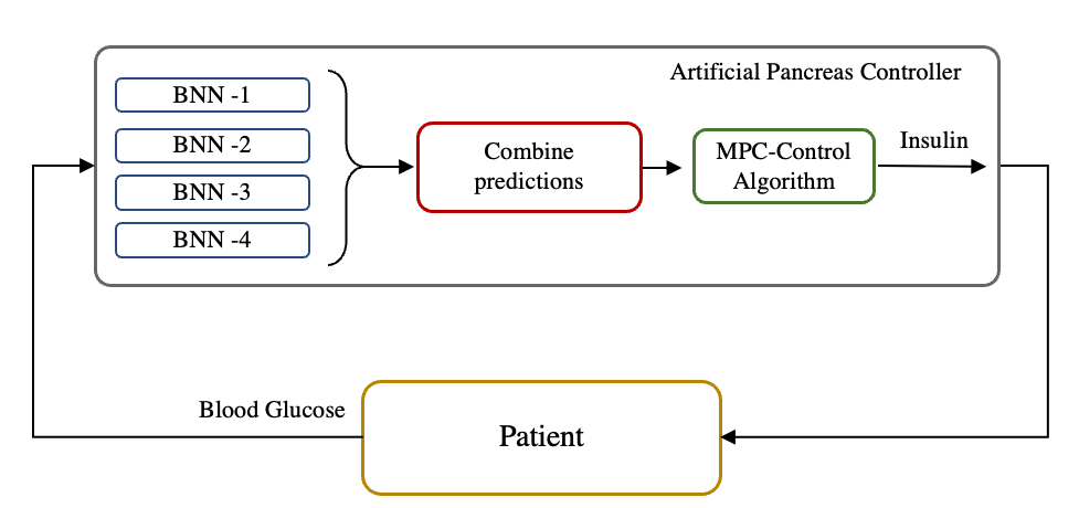
External insulin delivery is accomplished by using an insulin pump controlled by the artificial pancreas software, which attempts to regulate the blood-glucose (BG) level of the patient within the euglycemic range of mg/dl [77]. Levels below mg/dl lead to hypoglycemia, which can lead to loss of consciousness, coma or even death. On the other hand, levels above mg/dl lead to a condition called ketoacidosis, where the body can break down fat due to lack of insulin, and lead to build up of ketones. In order to treat this situation, patients receive external insulin delivery through insulin pumps. Artificial Pancreas (AP) systems can remedy this situation by measuring the blood glucose level, and automatically injecting insulin into the blood stream. Thus, we define the unsafe regions of the space as , where is the BG value at time . This is the shaded region in Figure 10.

Neural Network Models and Controller. Deep Neural Networks are effective in capturing the BG-insulin dynamics for personalized medical devices [77]. This allows for improved device performance. Even though standard Feedforward Neural Networks can be used, Bayesian Neural Networks (BNNs), and especially a collection of multiple BNNs, offer a better alternative towards uncertainty aware predictions. Here, we test the ramifications of these prediction sets, when used inside an online receding horizon control scheme for insulin delivery. We use the standard MPC control scheme for this purpose, well-known in the literature [42]. More formally, let and be the blood-glucose and insulin values at time , respectively. We denote the finite length trajectory of length as , and . An uncertainty aware model computes the triplet , where is the mean prediction output, and are the lower and upper predictions of the glucose value, respectively. By design, it is true that . A model predictive control algorithm – whose cost function we denote by – solves .
After every time step, the control algorithm picks the first insulin input as the insulin bolus for the patient, and discards the rest. Cost function takes into account three factors, (i) Distance of the mean prediction level at each time step from a target value of mg/dl, (ii) Distance of upper and lower predictions ( and ) from the unsafe regions of the state space and , and (iii) Total insulin injected .
Starting with some initial glucose value , we measure the performance of the artificial pancreas controller as the fraction of time it spends in the unsafe regions,
where denotes the indicator function. A lower value is more desirable. We compare EBNN and CBDL as different realizations of the model .
Distribution Shift using Meals. A well known problem with learned models is distribution shift. Bayesian Neural Networks can address this issue by apprising the end user of the increased uncertainty. For regression models of the type described above, this appears as larger prediction intervals . The artificial pancreas controller can run into this situation in the following way: the insulin-glucose time series data collected for training the data-driven model can be without meals, while at test time the patient can have meals. This creates a distribution shift between the training and test time data. Fortunately, the UVa-Padova simulator [33] allows us to create datasets with and without meal inputs. In this case study, the training data was obtained by randomly initializing the BG value in the range , and simulating the patient for minutes. The controller was executed at minutes intervals. At test time the patient was supplied meals at specific time intervals (for details, see Appendix J). This creates a significant distribution shift since meals are effectively an unknown variable which can affect the system state. However, from the controller’s perspective this is practical, since patients can have unannounced meals.
Results and Discussion. To capture the difference in performance between EBNN and CBDL, we compute . Both and depend on interval ; for EBNN, this latter corresponds to the -level HDR associated with EBNN distribution , while for CBDL it corresponds to the IHDR . We consider one case in which CBDL is trained using a credal prior set and only one likelihood (we choose different seeds which initialize the prior distributions but we keep the same architecture for the BNNs), and another case in which we do the opposite (we use the same seed and different architectures).
We report , across different choices in Table 7. We observe that for lower values of (or equivalently, for larger values of , e.g. and ) the gains of CBDL are more pronounced. This means that when larger significance levels need to be ensured, CBDL is to be preferred to ensemble of BNNs. As discussed before, the CBDL procedure considers all the infinitely many possible priors that can be expressed as a convex combination of the priors that the user specifies at the beginning of the analysis. The same holds for the likelihoods. While this results in a more conservative estimate as compared to the EBNN framework, CBDL produces controllers which respect the safety limits better. To see that CBDL is more conservative than EBNN, notice that when combining predictive distributions from multiple BNNs, CBDL combines the predictions via a finitely generated credal set (FGCS) whose extrema are the individual distributions. On the contrary, an EBNN takes an average of the individual distributions to compute the ensemble distribution . The union of the HDRs of the predictive distributions is more conservative (i.e., broader) than the HDR of the single ensemble distribution. While the approach by EBNN seems like a reasonable choice on the surface, it falls short in capturing the uncertainty necessary for the downstream task. For more details on this case study, see Appendix J.
| Varying Seeds | -5.8% | 5.5% | 0.6% |
| Varying | |||
| Architectures | -6.6% | 0.9% | 0.3% |
5. Related Work
In [30], the authors introduce credal classifiers (CCs) as a generalization of classifiers based on Bayesian networks. Unlike CCs, CBDL does not require independence assumptions between non-descendant, non-parent variables. In addition, CBDL avoids NP-hard complexity issues of searching for optimal structure in the space of Bayesian networks [27]. In [85], an epistemic convolutional neural network (ECNN) is developed that explicitly models the epistemic uncertainty induced by training data of limited size and quality. A clear distinction is that ECNNs measure uncertainty in target-level representations whereas CBDL identifies the uncertainty measure on the output space . Despite the merit of their work, we believe CBDL achieves greater generality, since it is able to quantify both aleatoric and epistemic predictive uncertainties, and is applicable to problems beyond classification. For a review of the state of the art concerning the distinction between EU and AU we refer to [59] and to [85]. We also point out how CBDL has been recently used to solve prior-likelihood conflicts in Bayesian statistics [87]. Further references can be found in Appendix L.
We also point out how there exist other efficient methods which perform approximate Variational Inference via dropouts in deep neural networks [69, 48]. As mentioned at the end of section 3.1, we can easily adapt CBDL to use such dropout approximations in Steps 3-4 of Algorithm 1. Since our contribution is centered around how different predictions can be combined via an FGCS, we used the de-facto standard for performing inference on BNNs, which is based on off-the-shelf VI techniques. In the future, we plan to study the effect on computational complexity and uncertainty quantification capability of a CBDL procedure that approximates posterior and predictive distributions via dropout.
We do not consider Bayesian Model Averaging (BMA) as a baseline for CBDL for two main reasons. First, BMA applied to deep learning needs to implement full batch Hamiltonian Monte Carlo in order to get to the true posterior [61]. Given the number of parameters in modern deep learning architectures – in the order of millions – this is realistically possible at an experimental level only to labs with access to industry scale computational resources. In order to be practically relevant, we limit our experiments to the more well-understood realm of Variational Inference on BNNs. In addition, [60] show the pitfalls of BMA in the context of Bayesian Neural Networks, a further reason not to use a Highest Density Region resulting from BMA as a baseline for CBDL. Such pitfalls are related to the fact that BMA can be seen as a model featuring second-order distributions, i.e. distributions over distributions. In particular, the distribution in (1) is a second order distribution. These types of models have been recently shown to suffer from major pitfalls when used to quantify predictive EU due to their sensitivity to regularization parameters, and to underestimate predictive AU [7, 94, 66].
6. Conclusion
We presented CBDL, a procedure that can be seen as a non-condensed, uncountably infinite ensemble of BNNs, carried out using only finitely many elements. It allows to distinguish between predictive AU and EU, and to quantify them. We showed how it can be used to specify a set of outputs – the IHDR – that enjoys probabilistic guarantees. We showed empirically that it improves on the Bayesian state of the art at gauging predictive AU and EU, and we also demonstrated its downstream tasks capabilities.
We point out how a region that improves on , meaning that it would be tighter, is
where , and is the largest constant such that . The problem with is that, while the highest density regions associated with the predictive distributions in can be computed using off-the-shelf tools, calculating and would have been much more computationally expensive. In addition, it would have required to come up with a new technique to find and . We defer studying this to future work.
We also plan to apply CBDL to continual learning to overcome the curse of dimensionality and to capture an agent’s preference over the tasks to perform, similarly to [84], and to active learning, to be able to sample from the regions of the state space exhibiting the highest epistemic uncertainty, similarly to [41].
Furthermore, we intend to relate CBDL to Bayesian Model Selection (BMS) [49]. This latter suffers from the same problem as “regular” Bayesian inference. That is, while it tries to come up with a sophisticate prior that induces shrinkage, it still relies on the “correctness” of that prior, i.e. on correctly specifying the prior’s parameters. In the future, an interesting way of combining CBDL with BMS will be to use a finite number of regularized horseshoe priors, as suggested by [49, Section 3.2], as extreme elements of the prior credal set.
We also call attention to the fact that CBDL is a model-based approach. The relationship with model-free approaches such as conformal prediction [103] will be the object of future studies. In particular, we are interested in finding in which cases IHDRs are narrower than conformal regions, and vice versa, and which credal sets give rise to IHDRs enjoying the same probabilistic guarantees as conformal regions.
Finally, we point out how one possible way of easing the burden of the combinatorial task in Step 3 of Algorithm 1 is to specify a prior credal set whose size strikes the perfect balance between being “vague enough” so that we do not underestimate the EU, and being “small enough” so that CBDL is actually implementable. We suspect conjugacy of the priors may play a key role in this endeavor. Because of its centrality, we defer the study of “optimal prior credal sets” to future work. We also point out how an evidential approach [3, 26, 37, 38, 102] – at least in classification problems – could allows us to bypass the bottleneck in Algorithm 1 by merging an imprecise probabilistic approach, with some tricks resulting from smartly choosing our priors.
A CBDL-adjacent research question of great interest pertaining ensemble learning, then, is how do single components of an ensemble contribute to the quantification of the “global predictive EU” faced by the agent. When the uncertainty captured by an ensemble is distilled into only one distribution, there could indeed be “uncertainty spills”, like when one pours water in a glass too hastily, and some finishes on the table instead of in the glass. This remains an unexplored venue in the uncertainty quantification community.
References
- [1] Joaquín Abellán, George Jiří Klir, and Serafín Moral. Disaggregated total uncertainty measure for credal sets. International Journal of General Systems, 1(35):29–44, 2006.
- [2] Joaquín Abellán and Serafín Moral. A non-specificity measure for convex sets of probability distributions. International Journal of Uncertainty, Fuzziness and Knowledge-Based Systems, 8(3):357–367, 2000.
- [3] Alexander Amini, Wilko Schwarting, Ava Soleimany, and Daniela Rus. Deep evidential regression. In H. Larochelle, M. Ranzato, R. Hadsell, M.F. Balcan, and H. Lin, editors, Advances in Neural Information Processing Systems, volume 33, pages 14927–14937. Curran Associates, Inc., 2020.
- [4] Thomas Augustin, Frank P.A. Coolen, Gert De Cooman, and Matthias C.M. Troffaes, editors. Introduction to imprecise probabilities. Wiley Series in Probability and Statistics. John Wiley and Sons, 2014.
- [5] David Avis and Komei Fukuda. Reverse search for enumeration. Discrete Applied Mathematics, 65:21–46, 1996.
- [6] Rina Foygel Barber, Emmanuel J. Candès, Aaditya Ramdas, and Ryan J. Tibshirani. Conformal prediction beyond exchangeability. The Annals of Statistics, 51(2):816 – 845, 2023.
- [7] Viktor Bengs, Eyke Hüllermeier, and Willem Waegeman. Pitfalls of epistemic uncertainty quantification through loss minimisation. In Alice H. Oh, Alekh Agarwal, Danielle Belgrave, and Kyunghyun Cho, editors, Advances in Neural Information Processing Systems, 2022.
- [8] James O. Berger. The robust Bayesian viewpoint. In Joseph B. Kadane, editor, Robustness of Bayesian Analyses. Amsterdam : North-Holland, 1984.
- [9] Jose M. Bernardo. Reference posterior distributions for Bayesian inference. Journal of the Royal Statistical Society: Series B, 41(2):113–128, 1979.
- [10] George E. P. Box. Science and statistics. Journal of the American Statistical Association, 71(356):791–799, 1976.
- [11] Andrey G. Bronevich and Igor N. Rozenberg. Generalized Hartley measures on credal sets. In Andrés Cano, Jasper De Bock, Enrique Miranda, and Serafín Moral, editors, Proceedings of the Twelveth International Symposium on Imprecise Probability: Theories and Applications, volume 147 of Proceedings of Machine Learning Research, pages 32–41. PMLR, 2021.
- [12] Yuhang Cai and Lek-Heng Lim. Distances between probability distributions of different dimensions. IEEE Transactions on Information Theory, 68(6):4020–4031, 2022.
- [13] Michele Caprio. Refined Pinsker’s and reverse Pinsker’s inequalities for probability distributions of different dimensions. IEEE Access, 10:116425–116431, 2022.
- [14] Michele Caprio. Imprecise Markov Semigroups and their Ergodicity, 2024.
- [15] Michele Caprio. Optimal Transport for -Contaminated Credal Sets, 2024.
- [16] Michele Caprio and Ruobin Gong. Dynamic precise and imprecise probability kinematics. In Enrique Miranda, Ignacio Montes, Erik Quaeghebeur, and Barbara Vantaggi, editors, Proceedings of the Thirteenth International Symposium on Imprecise Probability: Theories and Applications, volume 215 of Proceedings of Machine Learning Research, pages 72–83. PMLR, 11–14 Jul 2023.
- [17] Michele Caprio, Kuk Jin Jang, Souradeep Dutta, Shireen Manchingal, Fabio Cuzzolin, Oleg Sokolsky, and insup Lee. Credal and interval deep evidential classification. Technical Reports of the PRECISE Center, 2024.
- [18] Michele Caprio and Sayan Mukherjee. Concentration inequalities and optimal number of layers for stochastic deep neural networks. IEEE Access, 11:38458–38470, 2023.
- [19] Michele Caprio and Sayan Mukherjee. Ergodic theorems for dynamic imprecise probability kinematics. International Journal of Approximate Reasoning, 152:325–343, 2023.
- [20] Michele Caprio and Sayan Mukherjee. Extended probabilities and their application to statistical inference, chapter 2. World Scientific, 2023.
- [21] Michele Caprio and Sayan Mukherjee. Finite admixture models: a bridge with stochastic geometry and choquet theory. Available at arXiv:2002.08409, 2023.
- [22] Michele Caprio, Yusuf Sale, Eyke Hüllermeier, and Insup Lee. A Novel Bayes’ Theorem for Upper Probabilities. In Fabio Cuzzolin and Maryam Sultana, editors, Epistemic Uncertainty in Artificial Intelligence, pages 1–12, Cham, 2024. Springer Nature Switzerland.
- [23] Michele Caprio and Teddy Seidenfeld. Constriction for sets of probabilities. In Enrique Miranda, Ignacio Montes, Erik Quaeghebeur, and Barbara Vantaggi, editors, Proceedings of the Thirteenth International Symposium on Imprecise Probability: Theories and Applications, volume 215 of Proceedings of Machine Learning Research, pages 84–95. PMLR, 11–14 Jul 2023.
- [24] Michele Caprio, Maryam Sultana, Eleni Elia, and Fabio Cuzzolin. Credal learning theory, 2024.
- [25] Simone Cerreia-Vioglio, Fabio Maccheroni, and Massimo Marinacci. Ergodic theorems for lower probabilities. Proceedings of the American Mathematical Society, 144:3381–3396, 2015.
- [26] Bertrand Charpentier, Daniel Zügner, and Stephan Günnemann. Posterior network: Uncertainty estimation without OOD samples via density-based pseudo-counts. In H. Larochelle, M. Ranzato, R. Hadsell, M.F. Balcan, and H. Lin, editors, Advances in Neural Information Processing Systems, volume 33, pages 1356–1367. Curran Associates, Inc., 2020.
- [27] David M. Chickering, David Heckerman, and Christopher Meek. Large-sample learning of Bayesian networks is NP-hard. The Journal of Machine Learning Research, 5:1287–1330, 2004.
- [28] Adam D. Cobb, Michael D. Himes, Frank Soboczenski, Simone Zorzan, Molly D. O’Beirne, Atılım Güneş Baydin, Yarin Gal, Shawn D. Domagal-Goldman, Giada N. Arney, Daniel Angerhausen, and 2018 NASA FDL Astrobiology Team II. An ensemble of Bayesian neural networks for exoplanetary atmospheric retrieval. The Astronomical Journal, 158(1):33, 2019.
- [29] Frank P. A. Coolen. Imprecise highest density regions related to intervals of measures. Memorandum COSOR, 9254, 1992.
- [30] Giorgio Corani, Alessandro Antonucci, and Marco Zaffalon. Bayesian Networks with Imprecise Probabilities: Theory and Application to Classification, chapter 4 of Data Mining: Foundations and Intelligent Paradigms: Volume 1: Clustering, Association and Classification, pages 49–93. Berlin, Germany : Springer, 2012.
- [31] Fabio G. Cozman. Credal networks. Artificial Intelligence, 120(2):199–233, 2000.
- [32] Fabio Gagliardi Cozman. Credal networks. Artificial Intelligence, 120:199–233, 2000.
- [33] Chiara Dalla Man, Francesco Micheletto, Dayu Lv, Marc D. Breton, Boris Kovatchev, and Claudio Cobelli. The UVA/PADOVA type 1 diabetes simulator: New features. Journal of Diabetes Science and Technology, 8(1):26–34, 2013.
- [34] George B. Dantzig. Linear Programming and Extensions. Princeton University Press, 1963.
- [35] Bruno de Finetti. Theory of Probability, volume 1. New York : Wiley, 1974.
- [36] Bruno de Finetti. Theory of Probability, volume 2. New York : Wiley, 1975.
- [37] Thierry Denœux. An evidential neural network model for regression based on random fuzzy numbers. In Sylvie Le Hégarat-Mascle, Isabelle Bloch, and Emanuel Aldea, editors, Belief Functions: Theory and Applications, pages 57–66, Cham, 2022. Springer International Publishing.
- [38] Thierry Denœux. Quantifying prediction uncertainty in regression using random fuzzy sets: the ENNreg model. IEEE Transactions on Fuzzy Systems, pages 1–10, 2023.
- [39] Stefan Depeweg, Jose-Miguel Hernandez-Lobato, Finale Doshi-Velez, and Steffen Udluft. Decomposition of uncertainty in Bayesian deep learning for efficient and risk-sensitive learning. In International Conference on Machine Learning, pages 1184–1193. PMLR, 2018.
- [40] Didier Dubois and Eyke Hüllermeier. Comparing probability measures using possibility theory: A notion of relative peakedness. International Journal of Approximate Reasoning, 45(2):364–385, 2007. Eighth European Conference on Symbolic and Quantitative Approaches to Reasoning with Uncertainty (ECSQARU 2005).
- [41] Souradeep Dutta, Michele Caprio, Vivian Lin, Matthew Cleaveland, Kuk Jin Jang, Ivan Ruchkin, Oleg Sokolsky, and Insup Lee. Distributionally robust statistical verification with imprecise neural networks. arXiv preprint arXiv:2308.14815, 2023.
- [42] Souradeep Dutta, Taisa Kushner, and Sriram Sankaranarayanan. Robust data-driven control of artificial pancreas systems using neural networks. In Milan Češka and David Šafránek, editors, Computational Methods in Systems Biology, pages 183–202, Cham, 2018. Springer International Publishing.
- [43] Daniel Ellsberg. Risk, ambiguity, and the Savage axioms. The Quarterly Journal of Economics, 75(4):643–669, 1961.
- [44] Mohammed Fellaji and Frédéric Pennerath. The epistemic uncertainty hole: an issue of bayesian neural networks. Available at arXiv:2407.01985, 2024.
- [45] Emlyn Flint, Florence Chikurunhe, and Anthony Seymour. Regime-based tactical allocation for equity factors and balanced portfolios. SSRN Electronic Journal, 01 2017.
- [46] Benoît Fortin, Samir Hachour, and François Delmotte. Multi-target PHD tracking and classification using imprecise likelihoods. International Journal of Approximate Reasoning, 90:17–36, 2017.
- [47] Vincent Fortuin, Adrià Garriga-Alonso, Mark van der Wilk, and Laurence Aitchison. BNNpriors: A library for bayesian neural network inference with different prior distributions. Software Impacts, 9:100079, 2021.
- [48] Yarin Gal and Zoubin Ghahramani. Dropout as a bayesian approximation: Representing model uncertainty in deep learning, 2016.
- [49] Soumya Ghosh, Jiayu Yao, and Finale Doshi-Velez. Model selection in Bayesian neural networks via horseshoe priors. Journal of Machine Learning Research, 20(182):1–46, 2019.
- [50] Isaac Gibbs, John J. Cherian, and Emmanuel J. Candès. Conformal prediction with conditional guarantees. Available at arXiv:2305.12616, 2023.
- [51] Itzhak Gilboa and Massimo Marinacci. Ambiguity and the Bayesian paradigm. In Daron Acemoglu, Manuel Arellano, and Eddie Dekel, editors, Advances in Economics and Econometrics, Tenth World Congress, volume 1. Cambridge : Cambridge University Press, 2013.
- [52] Ethan Goan and Clinton Fookes. Bayesian Neural Networks: An Introduction and Survey, pages 45–87. Cham, Switzerland : Springer International Publishing, 2020.
- [53] Ruobin Gong and Xiao-Li Meng. Judicious judgment meets unsettling updating: dilation, sure loss, and Simpson’s paradox. Statistical Science, 36(2):169–190, 2021.
- [54] Chuan Guo, Geoff Pleiss, Yu Sun, and Kilian Q Weinberger. On calibration of modern neural networks. In International conference on machine learning, pages 1321–1330. PMLR, 2017.
- [55] Dan Hendrycks and Thomas G. Dietterich. Benchmarking neural network robustness to common corruptions and perturbations. CoRR, abs/1903.12261, 2019.
- [56] Paul Hofman, Yusuf Sale, and Eyke Hüllermeier. Quantifying aleatoric and epistemic uncertainty: A credal approach. In ICML 2024 Workshop on Structured Probabilistic Inference & Generative Modeling, 2024.
- [57] Peter J. Huber and Elvezio M. Ronchetti. Robust statistics. Wiley Series in Probability and Statistics. Hoboken, New Jersey : Wiley, 2nd edition, 2009.
- [58] Rob J. Hyndman. Computing and graphing highest density regions. The American Statistician, 50(2):120–126, 1996.
- [59] Eyke Hüllermeier and Willem Waegeman. Aleatoric and epistemic uncertainty in machine learning: an introduction to concepts and methods. Machine Learning, 3(110):457–506, 2021.
- [60] Pavel Izmailov, Patrick Nicholson, Sanae Lotfi, and Andrew G Wilson. Dangers of bayesian model averaging under covariate shift. In M. Ranzato, A. Beygelzimer, Y. Dauphin, P.S. Liang, and J. Wortman Vaughan, editors, Advances in Neural Information Processing Systems, volume 34, pages 3309–3322. Curran Associates, Inc., 2021.
- [61] Pavel Izmailov, Sharad Vikram, Matthew D. Hoffman, and Andrew Gordon Wilson. What are bayesian neural network posteriors really like? CoRR, abs/2104.14421, 2021.
- [62] Pavel Izmailov, Sharad Vikram, Matthew D Hoffman, and Andrew Gordon Gordon Wilson. What are Bayesian neural network posteriors really like? In Marina Meila and Tong Zhang, editors, Proceedings of the 38th International Conference on Machine Learning, volume 139, pages 4629–4640. PMLR, 2021.
- [63] Harold Jeffreys. An invariant form for the prior probability in estimation problems. Proceedings of the Royal Society A, 186(1007):453–461, 1946.
- [64] Laurent Valentin Jospin, Hamid Laga, Farid Boussaid, Wray Buntine, and Mohammed Bennamoun. Hands-on Bayesian neural networks – A tutorial for deep learning users. IEEE Computational Intelligence Magazine, 17(2):29–48, 2022.
- [65] Ngumbang Juat, Mike Meredith, and John Kruschke. Package ‘hdinterval’, 2022. Accessed on May 9, 2023.
- [66] Mira Juergens, Nis Meinert, Viktor Bengs, Eyke Hüllermeier, and Willem Waegeman. Is epistemic uncertainty faithfully represented by evidential deep learning methods? In Forty-first International Conference on Machine Learning, 2024.
- [67] Sanyam Kapoor, Wesley J Maddox, Pavel Izmailov, and Andrew Gordon Wilson. On uncertainty, tempering, and data augmentation in bayesian classification. arXiv preprint arXiv:2203.16481, 2022.
- [68] Ramneet Kaur, Xiayan Ji, Souradeep Dutta, Michele Caprio, Yahan Yang, Elena Bernardis, Oleg Sokolsky, and Insup Lee. Using semantic information for defining and detecting OOD inputs. Available at arXiv:2302.11019, 2023.
- [69] Alex Kendall and Yarin Gal. What uncertainties do we need in bayesian deep learning for computer vision? Advances in neural information processing systems, 30, 2017.
- [70] Jang-Hyun Kim, Wonho Choo, and Hyun Oh Song. Puzzle mix: Exploiting saliency and local statistics for optimal mixup. In Hal Daumé III and Aarti Singh, editors, Proceedings of the 37th International Conference on Machine Learning, volume 119 of Proceedings of Machine Learning Research, pages 5275–5285. PMLR, 13–18 Jul 2020.
- [71] John Klein, Christèle Lecomte, and Pierre Miché. Hierarchical and conditional combination of belief functions induced by visual tracking. International Journal of Approximate Reasoning, 51(4):410–428, 2010.
- [72] Ranganath Krishnan, Mahesh Subedar, and Omesh Tickoo. MOPED: efficient priors for scalable variational inference in bayesian deep neural networks. CoRR, abs/1906.05323, 2019.
- [73] Ranganath Krishnan, Mahesh Subedar, and Omesh Tickoo. Specifying weight priors in Bayesian deep neural networks with empirical Bayes. Proceedings of the AAAI Conference on Artificial Intelligence, 34(04):4477–4484, April 2020.
- [74] Ranganath Krishnan and Omesh Tickoo. Improving model calibration with accuracy versus uncertainty optimization. In Advances in Neural Information Processing Systems, volume 33, pages 18237–18248. Curran Associates, Inc., 2020.
- [75] Alex Krizhevsky, Vinod Nair, and Geoffrey Hinton. CIFAR-10 (Canadian Institute for Advanced Research). Available at http://www.cs.toronto.edu/ kriz/cifar.html, 2009.
- [76] Meelis Kull and Peter A. Flach. Reliability Maps: A Tool to Enhance Probability Estimates and Improve Classification Accuracy. In Toon Calders, Floriana Esposito, Eyke Hüllermeier, and Rosa Meo, editors, Machine Learning and Knowledge Discovery in Databases, Lecture Notes in Computer Science, pages 18–33, Berlin, Heidelberg, 2014. Springer.
- [77] Taisa Kushner, David Bortz, David M. Maahs, and Sriram Sankaranarayanan. A data-driven approach to artificial pancreas verification and synthesis. In Proceedings of the 9th ACM/IEEE International Conference on Cyber-Physical Systems, ICCPS ’18, pages 242–252. IEEE Press, 2018.
- [78] Jouko Lampinen and Aki Vehtari. Bayesian approach for neural networks - review and case studies. Neural Networks, 4:257–274, 2001.
- [79] Daniel Lassiter. Representing credal imprecision: from sets of measures to hierarchical Bayesian models. Philosophical Studies, 177(6):1463–1485, 2020.
- [80] Yann Lecun, Léon Bottou, Yoshua Bengio, and Patrick Haffner. Gradient-based learning applied to document recognition. Proceedings of the IEEE, 86(11):2278–2324, 1998.
- [81] Peter Lenk and Bryan Orme. The value of informative priors in Bayesian inference with sparse data. Journal of Marketing Research, 46(6):832–845, 2009.
- [82] Isaac Levi. The Enterprise of Knowledge. London, UK : MIT Press, 1980.
- [83] Vivian Lin, Kuk Jin Jang, Souradeep Dutta, Michele Caprio, Oleg Sokolsky, and Insup Lee. DC4L: Distribution shift recovery via data-driven control for deep learning models. In Alessandro Abate, Mark Cannon, Kostas Margellos, and Antonis Papachristodoulou, editors, Proceedings of the 6th Annual Learning for Dynamics and Control Conference, volume 242 of Proceedings of Machine Learning Research, pages 1526–1538. PMLR, 15–17 Jul 2024.
- [84] Pengyuan Lu, Michele Caprio, Eric Eaton, and Insup Lee. Zero-shot task preference addressing enabled by imprecise Bayesian continual learning. Available at arXiv:2305.14782, 2023.
- [85] Shireen Kudukkil Manchingal and Fabio Cuzzolin. Epistemic deep learning. Available at arxiv:2206.07609, 2022.
- [86] Massimo Marinacci and Luigi Montrucchio. Introduction to the mathematics of ambiguity. In Itzhak Gilboa, editor, Uncertainty in economic theory: a collection of essays in honor of David Schmeidler’s 65th birthday. London : Routledge, 2004.
- [87] Alexander Marquardt, Julian Rodemann, and Thomas Augustin. An empirical study of prior-data conflicts in Bayesian neural networks. Poster presented at 13th International Symposium on Imprecise Probabilities: Theories and Applications (ISIPTA) 2023, 2023.
- [88] Jacques Paul Migne. De coelesti hierarchia. In Patrologia Graeca, volume 3. Paris : Imprimerie Catholique, 1857.
- [89] Enrique Miranda and Ignacio Montes. Centroids of the core of exact capacities: a comparative study. Annals of Operations Research, 321:409–449, 2023.
- [90] Norman Mu and Justin Gilmer. MNIST-C: A robustness benchmark for computer vision. CoRR, abs/1906.02337, 2019.
- [91] Bálint Mucsányi, Michael Kirchhof, and Seong Joon Oh. Benchmarking uncertainty disentanglement: Specialized uncertainties for specialized tasks. Available at arXiv:2402.19460, 2024.
- [92] Yuval Netzer, Tao Wang, Adam Coates, Alessandro Bissacco, Bo Wu, and Andrew Y. Ng. Reading digits in natural images with unsupervised feature learning. In NIPS Workshop on Deep Learning and Unsupervised Feature Learning 2011, 2011.
- [93] Matthew O’Kelly, Hongrui Zheng, Dhruv Karthik, and Rahul Mangharam. F1TENTH: An Open-source Evaluation Environment for Continuous Control and Reinforcement Learning. In Proceedings of the NeurIPS 2019 Competition and Demonstration Track, pages 77–89. PMLR, 2020.
- [94] Deep Shankar Pandey and Qi Yu. Learn to accumulate evidence from all training samples: Theory and practice. In Andreas Krause, Emma Brunskill, Kyunghyun Cho, Barbara Engelhardt, Sivan Sabato, and Jonathan Scarlett, editors, Proceedings of the 40th International Conference on Machine Learning, volume 202 of Proceedings of Machine Learning Research, pages 26963–26989. PMLR, 23–29 Jul 2023.
- [95] Sangdon Park, Osbert Bastani, Nikolai Matni, and Insup Lee. PAC confidence sets for deep neural networks via calibrated prediction. In 8th International Conference on Learning Representations, 2020.
- [96] Luis Raul Pericchi. Sets of prior probabilites and bayesian robustness. Documentation Section on the website of the Society for Imprecise Probability Theory and Applications (SIPTA), 1998.
- [97] Matthew Reimherr, Xiao-Li Meng, and Dan L. Nicolae. Prior sample size extensions for assessing prior impact and prior-likelihood discordance. Journal of the Royal Statistical Society: Series B (Statistical Methodology), 83(3):413–437, 2021.
- [98] Hippolyt Ritter, Aleksandar Botev, and David Barber. A scalable laplace approximation for neural networks. In International Conference on Learning Representations, 2018.
- [99] Yusuf Sale, Viktor Bengs, Michele Caprio, and Eyke Hüllermeier. Second-order uncertainty quantification: A distance-based approach. In Ruslan Salakhutdinov, Zico Kolter, Katherine Heller, Adrian Weller, Nuria Oliver, Jonathan Scarlett, and Felix Berkenkamp, editors, Proceedings of the 41st International Conference on Machine Learning, volume 235 of Proceedings of Machine Learning Research, pages 43060–43076. PMLR, 21–27 Jul 2024.
- [100] Yusuf Sale, Michele Caprio, and Eyke Hüllermeier. Is the volume of a credal set a good measure for epistemic uncertainty? In Robin J. Evans and Ilya Shpitser, editors, Proceedings of the Thirty-Ninth Conference on Uncertainty in Artificial Intelligence, volume 216 of Proceedings of Machine Learning Research, pages 1795–1804. PMLR, 31 Jul–04 Aug 2023.
- [101] Robin Senge, Stefan Bösner, Krzysztof Dembczyński, Jörg Haasenritter, Oliver Hirsch, Norbert Donner-Banzhoff, and Eyke Hüllermeier. Reliable classification: Learning classifiers that distinguish aleatoric and epistemic uncertainty. Information Sciences, 255:16–29, January 2014.
- [102] Murat Sensoy, Lance Kaplan, and Melih Kandemir. Evidential deep learning to quantify classification uncertainty. In S. Bengio, H. Wallach, H. Larochelle, K. Grauman, N. Cesa-Bianchi, and R. Garnett, editors, Advances in Neural Information Processing Systems, volume 31. Curran Associates, Inc., 2018.
- [103] Glenn Shafer and Vladimir Vovk. A tutorial on conformal prediction. Journal of Machine Learning Research, 9:371–421, 2008.
- [104] Marek Smieja and Jacek Tabor. Entropy of the mixture of sources and entropy dimension. IEEE Transactions on Information Theory, 58(5):2719–2728, 2012.
- [105] Lewis Smith and Yarin Gal. Understanding measures of uncertainty for adversarial example detection. arXiv preprint arXiv:1803.08533, 2018.
- [106] Bjørnar Tessem. Interval probability propagation. International Journal of Approximate Reasoning, 7(3):95–120, 1992.
- [107] D. Michael Titterington. Bayesian methods for neural networks and related models. Statistical Science, 19(1):128–139, 2004.
- [108] Krasymyr Tretiak, Georg Schollmeyer, and Scott Ferson. Neural network model for imprecise regression with interval dependent variables. Available at arXiv:2206.02467, 2022.
- [109] Matthias C.M. Troffaes and Gert de Cooman. Lower Previsions. Chichester, United Kingdom : John Wiley and Sons, 2014.
- [110] Renukanandan Tumu, Lars Lindemann, Truong Nghiem, and Rahul Mangharam. Physics Constrained Motion Prediction with Uncertainty Quantification, 2023. arXiv:2302.01060.
- [111] Vladimir Vovk, Alexander Gammerman, and Glenn Shafer. Algorithmic Learning in a Random World. Cham : Springer, second edition, 2022.
- [112] Peter Walley. Coherent lower (and upper) probabilities. Technical report, University of Warwick, Coventry, 1981.
- [113] Peter Walley. Statistical Reasoning with Imprecise Probabilities, volume 42 of Monographs on Statistics and Applied Probability. London : Chapman and Hall, 1991.
- [114] Hao Wang and Dit-Yan Yeung. A survey on Bayesian deep learning. ACM Computing Surveys, 53(5):1–37, 2021.
- [115] Larry A. Wasserman and Joseph B. Kadane. Bayes’ theorem for Choquet capacities. The Annals of Statistics, 18(3):1328–1339, 1990.
- [116] Lisa Wimmer, Yusuf Sale, Paul Hofman, Bernd Bischl, and Eyke Hüllermeier. Quantifying aleatoric and epistemic uncertainty in machine learning: Are conditional entropy and mutual information appropriate measures? In Robin J. Evans and Ilya Shpitser, editors, Proceedings of the Thirty-Ninth Conference on Uncertainty in Artificial Intelligence, volume 216 of Proceedings of Machine Learning Research, pages 2282–2292. PMLR, 31 Jul–04 Aug 2023.
- [117] Han Xiao, Kashif Rasul, and Roland Vollgraf. Fashion-MNIST: a novel image dataset for benchmarking machine learning algorithms. CoRR, abs/1708.07747, 2017.
- [118] Marco Zaffalon. The naive credal classifier. Journal of Statistical Planning and Inference, 105(1):5–21, 2002. Imprecise Probability Models and their Applications.
- [119] Fengshuo Zhang and Chao Gao. Convergence rates of variational posterior distributions. The Annals of Statistics, 48(4):2180 – 2207, 2020.
Appendix A Why do we need IPs?
The main motivations for working with credal sets are two. Let be the measurable space of interest.
- (i)
A single probability distribution does not suffice to represent ignorance in the sense of lack of knowledge; this is well documented in the literature, see e.g. [59] and references therein. Consider the example of complete ignorance (CI) in the case of a finite state space [59, Section 3.3]. In standard Bayesian analysis, CI is modeled in terms of the uniform distribution ; this is justified by Laplace’s “principle of indifference”. Then, however, it is not possible to distinguish between precise probabilistic knowledge about a random event – called prior indifference; think of the tossing of a fair coin – and a complete lack of knowledge due to an incomplete description of the experiment – called prior ignorance. Another problem is given by the additive nature of probability distributions. Consider again the example of a uniform distribution. First, let us observe that it is not invariant under reparametrization. In addition, if we model the ignorance about the length of the side of a cube in via a uniform measure on the interval , then this does not yield a uniform distribution of on , which suggests some degree of informedness about the cube’s volume. Finally, as pointed out in [113], if we ask a subject – even an expert – about their opinion regarding some events, it is much more likely that they will report interval of probabilities rather than single values.
- (ii)
Working with credal sets allows to achieve prior and likelihood robustness: realistically large sets of priors and of likelihoods are elicited. Using credal sets, the agent recognizes that prior beliefs and knowledge about the sampling model are limited and imprecise. Combining each pair of functions in and using Bayes’ rule, a class of posterior distributions – reflecting the updated state of uncertainty – is formed. If the available information is not sufficient to identify a unique posterior distribution, or a set of posteriors whose diameter is small, credal sets allow to represent indecision, thus leading to a less informative but more robust conclusions.2020 20 Here “diameter” has to be understood as the distance between upper and lower probability of event , for all .
Appendix B On the use of credal sets
Let us address a critique raised against the use of credal sets. [79] argues against the use of sets of probabilities to model an agent’s prior beliefs and their knowledge of the sampling model, while debating in favor of using hierarchical Bayesian models. As reported in [59, Secton 4.6.2], the argument against credal sets that is more cogent for the machine learning literature is that modeling a lack of knowledge in a set-based manner may hamper the possibility of inductive inference, up to a point where learning from empirical data is not possible any more. With this, we mean the following. As [96] points out, the natural candidate for a class of priors to represent complete ignorance is the class of all distributions. When this class leads to non-vacuous and useful conclusions, these are quite compelling and uncontroversial. It turns out that the posterior probabilities obtained from this class are vacuous, that is, their lower and upper bounds are and : no finite sample is enough to annihilate a sufficiently extreme prior belief. There is then a compromise to be made, and this is the compromise of near-ignorance. The near-ignorance class should be vacuous a priori in some respects, typically the ones that are the most important for the analysis at hand. This way of proceeding is labeled as arbitrary by [79], who instead advocates for the use of hierarchical Bayesian procedures. We find this critique not compelling, as during the analysis the job of the agent is to model reality: as pointed out in [59, Secton 5], statistical inference is not possible without underlying assumptions, and conclusions drawn from data are always conditional on those assumptions. If we were to work every time with the maximum level of generality, we would hardly be able to reach any conclusions. For example, in a statistical analysis we never consider the state of apparently possible states [113, section 2.1.2], that is, the one that contains all the states that are logically consistent with the available information. If we consider a coin toss, we let the state space be , certainly not heads, tails, coin landing on its edge, coin braking into pieces on landing, coin disappearing down a crack in the floor. The same holds for sets of probabilities: it makes much more sense to work with near-ignorance credal sets than to work with . A final reason to rebut the point in [79] is that the problems indicated in (i) in section A that make the use of the uniform prior distribution – often interpreted as representing epistemic uncertainty in standard Bayesian inference – at least debatable are inherited by hierarchical Bayesian modeling, as specified in [9, 59, 63]. Furthermore, a single distribution that is the result of a hierarchical Bayesian procedure is unable to gauge epistemic uncertainty [59].
B.1. Further notes on credal sets
As pointed out in [30, Section 3.3], there is a way of obtaining credal sets starting from sets of probability intervals; in addition, standard algorithms can compute the extreme elements of a credal set for which a probability interval has been provided [5]. However, the resulting number of extrema is exponential in the size of the possibility space [106].2121 21 Recall that the possibility space of a random variable is the space of the values it can take on. For this reason we prefer to specify prior and likelihood finitely generated credal sets instead.
The way credal sets behave after conditioning on new available evidence has been recently studied in [23], and a way of using credal sets in the open-world scenario (that is, when the support of the elements of the credal set can become larger as more data become available) is explored in [20]. Furthermore, the use of credal sets in statistical learning theory has been studied in [24], in computer vision in [14], and in optimal transport theory in [15].
Appendix C A further IP concept: the core
Let again be the measurable space of interest. Because of the conjugacy property of upper and lower probabilities, let us focus on upper probabilities only. We say that upper probability is concave if , for all . Recall that denotes the set of all probability measures on . Upper probability is compatible with the convex set [53]
where the second equality is a characterization [25, Page 3389]. Notice that the core is convex [86, Section 2.2]. We assume it is nonempty. Then, it is weak⋆-compact as a result of [86, Proposition 3].2222 22 Recall that in the weak⋆ topology, a net converges to if and only if , for all .
Since the core is convex, the set of extreme points of the core is well defined. It contains all the elements of the core that cannot be written as a convex combination of one another. The following important result is a consequence of [113, Theorem 3.6.2].
Theorem 9.
Suppose is nonempty. Then, the following holds.
- (a)
.
- (b)
is the closure in the weak⋆ topology of the convex hull of .
- (c)
If , for all , then , for all .
So in order to define an upper probability that setwise dominates the elements of it is enough to specify the extreme points of the core.
Appendix D A new Bayes’ theorem for IPs
We present Theorem 10, a result that – although appealing – does not lend itself well to be applied to the CBDL procedure. An extension of Theorem 10 is given in [22].
Call the parameter space of interest and assume it is Polish, that is, the topology for is complete, separable, and metrizable. This ensures that the set of probability measures on is Polish as well, where denotes the Borel -algebra for . Let be the set of all bounded, non-negative, -measurable functionals on . Call the sample space endowed with the product -algebra , where is the -algebra endowed to and is the -algebra endowed to . Let the agent elicit . Assume that each has density with respect to some -finite dominating measure on ; this represents the likelihood function for having observed data . We assume for now that , for all .
Let the agent specify a set of probabilities on . Then, compute , and consider ; it represents the agent’s initial beliefs.2323 23 Superscript “co” stands for convex and core. We assume that every has density with respect to some -finite dominating measure on , that is, . We require the agent’s beliefs to be represented by the core for two main reasons. The first, mathematical, one is to ensure that the belief set is compatible with the upper probability. The second, philosophical, one is the following [16, 19]. A criticism brought forward by [113, Section 2.10.4.(c)] is that, given an upper probability , there is no cogent reason for which the agent should choose a specific that is dominated by , or – for that matter – a collection of “plausible” probabilities. Because the core considers all (countably additive) probability measures that are dominated by , it is the perfect instrument to reconcile Walley’s behavioral and sensitivity analysis interpretations.
Let the agent compute , and consider ; it represents the set of plausible likelihoods. Let
| (4) |
and denote by and by , for all . Call
the class of posterior probabilities when the prior is in and the likelihood is in , and let , for all . Then, the following is a generalization of Bayes’ theorem in [115].
Theorem 10.
Suppose are nonempty. Then for all ,
| (5) |
provided that the ratio is well defined. Here, , and denotes the indicator function for . In addition, if is concave, then the inequality in (5) is an equality for all .
This result is particularly appealing because, given some assumptions, it allows to perform a (generalized) Bayesian update of a prior upper probability (PUP) by carrying out only one operation, even when the likelihood is ill specified so that a set of likelihoods is needed. We also have the following.
Lemma 11.
Suppose are nonempty. Then, if is concave, we have that is concave as well.
This lemma is important because it tells us that the generalized Bayesian update of Theorem 10 preserves concavity, and so it can be applied to successive iterations. If at time the PUP is concave, then the PUP at time – that is, the posterior upper probability at time – will be concave too. Necessary and sufficient conditions for a generic upper probability to be concave are given in [86, Section 5].
In the future, these results can be generalized to the case in which the elements of are unbounded using techniques in [109], and to the case in which the elements of are -valued, for some , since we never used specific properties of in our proofs.
Despite being attractive, the generalized Bayesian update of Theorem 10 hinges upon three assumptions, namely that and are both cores of an upper probability, that they are nonempty, and that the prior upper probability is concave. As the proverb goes, there is no free lunch. Having to check these assumptions, together with computing a supremum, an infimum, and the integrals in (5), makes Theorem 10 inadequate to be applied in the context of CBDL.
Appendix E Bounds on upper and lower entropy
In this section we find an upper bound for and a lower bound for that are extremely interesting. We first need to introduce three new concepts.
Definition 12.
Consider a set of probabilities on a generic measurable space . We say that lower probability is convex if , for all .
Then, let be either an upper or a lower probability, and consider a generic bounded measurable function on , that is, . We define the Choquet integral of with respect to as follows
where the right hand side integrals are (improper) Riemann integrals. If is additive, then the Choquet integral reduces to the standard additive integral.
Finally, if is uncountable, define for all
We call them lower and upper densities, respectively.
The following theorem gives the desired bounds.
Theorem 13.
Consider a set of probabilities on a generic measurable space . If is uncountable, assume that every is dominated by a -finite measure and that the Radon-Nikodym derivatives are continuous and bounded, for all . Define
and similarly
Then, and . In addition, if is concave, the first bound is tighter, and if is convex, the second bound is tighter.
Remark 14.
In [59, Section 4.6.1], the authors point out that [2] presents a generalization of the Hartley measure, called generalized Hartley measure , that can be used to disaggregate the total uncertainty captured by into aleatoric and epistemic uncertainties. We prefer not to introduce it in the present work because is defined based on the mass function of a belief function [53, Definition 2.4].2424 24 A belief function is a mathematical concept that should not be confused with the term “belief” we used throughout the paper to address the agent’s knowledge. This entails that the authors assume that lower probability associated with the set of probabilities of interest is a belief function, and so that for every collection such that , the following holds
for all . As it is immediate to see, this is assumption is not needed in the context of CBDL. Other ways of disentangling and quantifying AU and EU can be found e.g. in [100, 99]
Appendix F How to derive a predictive distribution
Suppose we performed a Bayesian updating procedure so to obtain posterior pdf . Recall that denotes the training set. We obtain the predictive distribution on as follows
where is the likelihood used to derive the posterior. Notice that the last equality comes from output only depending on input and parameter , and from having assumed (see section 2.1). From an applied point of view, a sample from is obtained as follows:
- (1)
specify input ;
- (2)
sample a parameter from the posterior, ;
- (3)
plug in the likelihood and sample .
Appendix G Aleatoric uncertainty check for -level IHDR
The diameter of is a function of the predictive aleatoric uncertainty (AU) faced by the agent.2525 25 Since the diameter is a metric concept, we assume that we can find a well-defined metric on . If that is not the case, we substitute the diameter with the notion of cardinality. If we want to avoid to perform the computation in Step 5 of Algorithm 1 only to discover that is “too large”, then we can add a “predictive AU check”.
At the beginning of the analysis, compute the lower entropy associated with the set of extreme elements of the VI-approximated predictive credal set . By (2), it is equal to the predictive aleatoric uncertainty encoded in . We then verify whether the lower entropy is “too high”. That is, if , for some , we want our procedure to abstain. This means that if the predictive aleatoric uncertainty in set is too high, then our procedure does not return any output set for input . The value of can be set equal to the entropy of the probability measures that are typically used in the context the agent works in. For example, in medical applications the agent may consider the entropy of a Normal distribution, while in financial applications the entropy of a distribution with fatter tails, such as a -distribution or a Cauchy. We call these reference values.
If we add this “predictive AU check”, at inference time (that is, before Step 4 of Algorithm 1), the agent needs to specify the pair of parameters .
Appendix H -level IHDR in a Classification setting
In classification problems, BNNs compute the probability vector
where we write to highlight the fact that is sampled from posterior , and then select the most likely class , where the ’s are the elements of .
When applied to a classification setting, the general procedure introduced in Algorithm 1 becomes the following. Recall that we denote by the cardinality of , and by the cardinality of . Assume that , that is, there are possible labels. Then, a VI-approximated predictive distribution in can be seen as -dimensional probability vector , where , for all , , and .
Now fix any and any , and define the partial order on as and , where , . This means that we can order the labels according to the probability that assigns to them: the first label will be the one having highest probability according to , the second label will have the second-highest probability according to , and so on.
Now order the label space according to so to obtain
This means that , for all , , for all (but ), and so on. That is, we order the labels from the most to the least likely according to .
Then, we call -level credible set according to , , the set
| (6) | ||||
for some . It corresponds to the -level HDR . Notice that we require because we may need to go slightly above level . Just as a toy example, we may have labels, of which would give a coverage, while would give a coverage of . If we are interested in the -level credible set, we ought to include the fourth label, thus yielding a coverage slightly higher than . The interpretation to is the following: it consists of the smallest collection of labels to which assigns probability of at least (that is, those having the highest probability of being the correct one for the new input ).
Finally, we call -level imprecise credible set, , the set
In turn, we have that .
Remark 15.
Notice that if a credible set of level is enough, then we can replace the left endpoint of the interval in (6) with , for some . Strictly speaking, in this case we obtain an -level credible set, which we denote by , where . Going back to our toy example, we will have a credible set with labels that yields a coverage of , so . In turn, this implies that the imprecise credible set will have a coverage of , that is, it will have level . We denote it by , where .
Appendix I Distance between a set of distributions and a single distribution having different dimensions
Many concepts in this section are derived from [12]. Let such that , and let . Call the set of probability measures on having finite -th moment, and the set of probability measures on having density with respect to some -finite dominating measure , . Let , where denotes the -dimensional identity matrix, and for any and any , define the following function
Let be the Borel -algebra on , and for any , define , the pushforward measure. Consider then two generic probability measures such that and , and call
Recall now the definition of -Wasserstein metric between two generic distributions defined on the same Euclidean space. Let , for some and some . Then, the -Wasserstein distance between them is defined as
where denotes the Euclidean distance, is interpreted as the essential supremum, and is the set of couplings between and , where is the projection onto the first coordinates, and is the projection to the last coordinates.
Recall then the definition of -divergence between two generic distributions defined on the same Euclidean space. Let , for some , and assume . Then, for any convex functional on such that , the -divergence between and is defined as
Aside from the Rényi divergence, the -divergence includes just about every known divergences as special case [12]. The following are the main results of this section.
Lemma 16.
Let such that , and let and be any convex functional on such that . Consider a generic and . Let and . Define
- •
, for all ;
- •
, for all ;
- •
;
- •
;
Then, for all the following holds
Lemma 17.
Let such that , and let and be any convex functional on such that . Consider a generic and . Let . Define
- •
, for all ;
- •
, for all ;
- •
;
- •
;
Then, for all the following holds
A visual representation of the application of Lemma 17 in the context of CBDL is given in Figure 11.
Appendix J Details on Artificial Pancreas Example
Artificial Pancreas Model. An important factor when designing the controller for an artificial pancreas is to adapt the insulin delivery algorithm to the particular details of the patient. This is because patients display a wide range of variability in their response to insulin, depending on age, Body Mass Index (BMI), and other physiological parameters. The Bayesian Neural Network models have hidden layers, with neurons each, for the case study with different seeds. This choice was informed by the experiments in [42]. For the case study with different architectures, we trained BNNs with different widths: , , , and . The horizon length is time steps, and the prediction horizon is steps into the future. The neural networks were trained for time steps, with a learning rate of , and batch size of using Mean-Field Variational Inference. The training dataset consisted of training samples, recorded without meals.
Controller. We implemented a simple model predictive controller, using an off-the-shelf implementation of the covariance matrix adaptation evolution strategy (CMA-ES). The model predictive control planning horizon was , with a fixed seed for the randomized solver.
Appendix K Other possible baselines for CBDL
Our experiments may seem like a type of belief tracking [46, 71]. Two comments are in order. First, this line of literature does not use deep learning techniques. Second, in these works the authors rely on Dempster-Shafer theory, a field in imprecise probability theory where lower probabilities are assumed to be belief functions, see Remark 14. We do not rely on this assumption in our work.
Appendix L Further related work
Modeling uncertainty has been a longstanding goal of ML/AI research and a variety of approaches have been developed for doing so [54, 95, 64]. Recently, emphasis has been placed on discerning between aleatoric and epistemic uncertainties [101, 76, 69]. In [108], the authors present an IP-based neural network which uses a regression technique based on probability intervals. Contrary to CBDL, their NN is rooted in the frequentist approach to imprecise probabilities [57].
In [85, Sections 2.1, 2.3], the authors focus on belief-functions-based classification methods. CBDL cannot be directly compared with these methodologies because (i) they do not require that the user expresses their knowledge via a belief function, but rather through a credal set; (ii) they can be used for regression and classification; (iii) they are rooted in Bayesian theory, as opposed to Dempster-Shafer theory. Other works in ML using a belief function approach are those from the field of evidential machine learning (EML), see e.g. [3, 26, 37, 38, 102] and references therein. Existing models mainly address clustering, classification, and regression problems. The reasons why CBDL cannot be directly compared with methods from the EML literature are (i) and (iii) above, the fact that EML methods are not (derived from) Bayesian ones, and that their definitions of AU and EU are slightly different from the canonical ones in ensemble deep learning.
Appendix M Proofs
Proof of Proposition 3.
If , for all , then it is immediate to see that , for all , since .
Suppose now that , for all . Then, we have that for all and all , . Pick now any . We can write it as , where , for all , , and . Pick then any ; we have
So . Because this holds for all and all , the claim is proven. ∎
Proof of Proposition 6.
The lower bound for the upper entropy of comes immediately from being a superset of .
Let us now prove the lower entropy equality. Let and . Pick any . By the definition of , there exists a collection of non-negative reals such that and . By the concavity of the entropy, we have that
Since was chosen arbitrarily and is finite, this implies that
In addition, we have that, since , . Combining this with the above result, we obtain
∎
Proof of Proposition 8.
Pick any metric on the space of probabilities on , and any . Because belongs to , can only be either equal to or smaller than . By the definition of , if , then . If instead , then . The proof is similar for a generic divergence div on . ∎
Proof of Theorem 10.
Assume are nonempty. Then, by [86, Proposition 3], they are weak⋆-compact. Pick any . Recall that we can rewrite the usual Bayes’ updating rule as
which is maximized when
is minimized. But
which proves the inequality in (5). Assume now that is concave. By [115, Lemma 1], we have that there exists such that
| (7) |
for all . In addition, by [115, Lemma 4], we have that for all and all , there exists a non-negative, upper semi-continuous function such that
| (8) | ||||
Let now . Notice that since is weak⋆-compact, by (4) so is . This implies that , since a compact set always contains its boundary, so as well, and in turn . Fix then any and put . It is immediate to see that is non-negative and upper semi-continuous. Then, by (8), we have that for all
| (9) | ||||
Combining (7) and(9), we obtain
| (10) | ||||
for all .
Pick now any and put
Choose any and . By (10) we have that and that . Recall that , and define . Then,
Since this holds for all , we have that
concluding the proof. ∎
Proof of Lemma 11.
[112, 115] show that concave upper probabilities are closed with respect to the generalized Bayes’ rule. In particular, this means that, if we let , for any fixed , if is concave, then for all
| (11) |
is concave. But since is weak⋆-compact (by our assumption and [86, Proposition 3]), by (4) so is . This implies that , since a compact set always contains its boundary. Call then . It is immediate to see that . Then, by (11) we have that if we call , it follows that
is concave, concluding the proof. ∎
Proof of Theorem 13.
Suppose is uncountable. First notice that, since we assumed to be continuous and bounded for all , then so is , for all , since composing a continuous function with a continuous and bounded one gives us a continuous and bounded function. This entails that the Choquet integrals of with respect to and are both well defined. In addition, being continuous and bounded, both and attain their infima and suprema thanks to Weierstrass’ extreme value theorem, for all . Hence, all the Choquet integrals used in this proof are well defined.
Then, we have the following
| (12) | ||||
| (13) | ||||
| (14) | ||||
| (15) | ||||
The inequality in (12) is true because for all ,
The inequality in (13) is a property of Choquet integrals taken with respect to upper probabilities [86]. The equality in (14) is true because for a generic function , we have that . Finally, the equality in (15) is true because the logarithm is a strictly increasing function. By [86, Theorem 38], if is concave, then inequality (13) holds with an equality, and so the bound is tighter.
The proof for is similar; we use the facts that
- •
, for all ;
- •
by [86],
(16) - •
for a generic function , ;
- •
Suppose now is at most countable; in this case, we do not need any assumptions to make the Choquet integrals well defined, since we will not deal with density functions. The following holds
| (17) | ||||
| (18) | ||||
| (19) | ||||
| (20) | ||||
The inequality in (17) comes from the well known fact that the sum of the suprema is at least equal to the supremum of the sum. The inequality in (18) comes from the fact that for differentiable functions, the product of the suprema is at least equal to the supremum of the product. The equality in (19) is true because for a generic function , we have that . Finally, the equality in (20) is true because the logarithm is a strictly increasing function. By [86, Theorem 38], if is concave, then inequality (17) holds with an equality, and so the bound is tighter.
The proof for is similar; we use the facts that
- •
the sum of the infima is at most equal to the infimum of the sum;
- •
for differentiable functions, the product of the infima is at most equal to the infimum of the product;
- •
for a generic function , ;
- •
by [86, Theorem 38], if is convex, then .
∎
Proof of Lemma 16.
Fix any and pick any . Because , then can only be either equal or smaller than . Now, if , then . If instead , then . This concludes the first part of the proof. Fix then any convex functional on such that ; the proof is similar for -divergences. ∎
Appendix N All Results: In-distribution and Out-of-distribution Evaluation
N.1. CIFAR-10 Results
| CBDL | Ensemble | BNN | |||||||||||||||||
| Epistemic | Aleatoric | Epistemic | Aleatoric | Epistemic | Aleatoric | ||||||||||||||
| Low | Med | High | Low | Med | High | Low | Med | High | Low | Med | High | Low | Med | High | Low | Med | High | ||
| CIFAR-10C | gaussian | 0.145 | 0.169 | 0.176 | 0.066 | 0.099 | 0.102 | 0.012 | 0.016 | 0.016 | 0.065 | 0.056 | 0.055 | 0.268 | 0.359 | 0.38 | 0.292 | 0.388 | 0.412 |
| shot noise | 0.129 | 0.158 | 0.174 | 0.053 | 0.084 | 0.104 | 0.01 | 0.014 | 0.016 | 0.069 | 0.061 | 0.055 | 0.224 | 0.315 | 0.378 | 0.249 | 0.342 | 0.409 | |
| speckle noise | 0.128 | 0.158 | 0.174 | 0.053 | 0.081 | 0.102 | 0.01 | 0.014 | 0.016 | 0.069 | 0.061 | 0.055 | 0.224 | 0.31 | 0.375 | 0.247 | 0.336 | 0.407 | |
| impulse | 0.134 | 0.161 | 0.174 | 0.052 | 0.085 | 0.118 | 0.011 | 0.015 | 0.017 | 0.069 | 0.059 | 0.051 | 0.231 | 0.338 | 0.423 | 0.257 | 0.364 | 0.454 | |
| defocus blur | 0.105 | 0.129 | 0.176 | 0.032 | 0.048 | 0.095 | 0.008 | 0.01 | 0.016 | 0.076 | 0.071 | 0.057 | 0.154 | 0.203 | 0.325 | 0.185 | 0.25 | 0.434 | |
| gaussian blur | 0.105 | 0.154 | 0.186 | 0.032 | 0.069 | 0.11 | 0.008 | 0.013 | 0.017 | 0.076 | 0.064 | 0.053 | 0.154 | 0.258 | 0.348 | 0.185 | 0.329 | 0.497 | |
| motion blur | 0.137 | 0.166 | 0.175 | 0.055 | 0.085 | 0.1 | 0.011 | 0.015 | 0.016 | 0.068 | 0.06 | 0.056 | 0.227 | 0.322 | 0.36 | 0.268 | 0.385 | 0.446 | |
| zoom blur | 0.148 | 0.161 | 0.176 | 0.063 | 0.077 | 0.1 | 0.012 | 0.014 | 0.016 | 0.066 | 0.062 | 0.056 | 0.253 | 0.287 | 0.338 | 0.318 | 0.365 | 0.457 | |
| snow | 0.131 | 0.157 | 0.163 | 0.05 | 0.077 | 0.086 | 0.01 | 0.014 | 0.015 | 0.07 | 0.062 | 0.059 | 0.221 | 0.31 | 0.337 | 0.242 | 0.326 | 0.355 | |
| fog | 0.104 | 0.122 | 0.154 | 0.033 | 0.045 | 0.09 | 0.008 | 0.009 | 0.013 | 0.076 | 0.072 | 0.06 | 0.155 | 0.199 | 0.321 | 0.187 | 0.246 | 0.397 | |
| brightness | 0.103 | 0.108 | 0.124 | 0.031 | 0.034 | 0.043 | 0.008 | 0.008 | 0.01 | 0.076 | 0.075 | 0.072 | 0.153 | 0.164 | 0.195 | 0.179 | 0.188 | 0.225 | |
| contrast | 0.107 | 0.145 | 0.165 | 0.035 | 0.066 | 0.148 | 0.008 | 0.012 | 0.017 | 0.075 | 0.065 | 0.046 | 0.162 | 0.265 | 0.419 | 0.197 | 0.342 | 0.69 | |
| elastic | 0.134 | 0.144 | 0.168 | 0.053 | 0.059 | 0.089 | 0.011 | 0.012 | 0.015 | 0.069 | 0.067 | 0.058 | 0.219 | 0.238 | 0.33 | 0.273 | 0.297 | 0.38 | |
| pixelate | 0.116 | 0.135 | 0.162 | 0.042 | 0.065 | 0.096 | 0.009 | 0.011 | 0.015 | 0.073 | 0.066 | 0.058 | 0.191 | 0.259 | 0.342 | 0.215 | 0.275 | 0.38 | |
| jpeg | 0.13 | 0.147 | 0.156 | 0.049 | 0.064 | 0.075 | 0.01 | 0.012 | 0.013 | 0.07 | 0.066 | 0.063 | 0.217 | 0.262 | 0.296 | 0.246 | 0.293 | 0.331 | |
| spatter | 0.117 | 0.145 | 0.147 | 0.041 | 0.065 | 0.062 | 0.009 | 0.012 | 0.012 | 0.073 | 0.065 | 0.066 | 0.191 | 0.279 | 0.266 | 0.216 | 0.299 | 0.291 | |
| saturate | 0.112 | 0.113 | 0.131 | 0.041 | 0.039 | 0.046 | 0.008 | 0.009 | 0.011 | 0.073 | 0.074 | 0.07 | 0.183 | 0.183 | 0.219 | 0.212 | 0.212 | 0.257 | |
| frost | 0.124 | 0.153 | 0.166 | 0.047 | 0.075 | 0.099 | 0.01 | 0.013 | 0.015 | 0.071 | 0.063 | 0.056 | 0.208 | 0.298 | 0.361 | 0.23 | 0.326 | 0.403 | |
| Epistemic | Aleatoric | Epistemic | Aleatoric | Epistemic | Aleatoric | ||||||||||||||
| In Dist-Clean | 0.102 | 0.031 | 0.008 | 0.076 | 0.151 | 0.179 | |||||||||||||
| Dataset | MNIST | 0.184 (1.801) | 0.142 (4.626) | 0.021 (2.723) | 0.044 (0.572) | 0.445 (2.95) | 0.772 (4.312) | ||||||||||||
| Fashion MNIST | 0.183 (1.791) | 0.147 (4.808) | 0.022 (2.822) | 0.042 (0.557) | 0.431 (2.861) | 0.811 (4.53) | |||||||||||||
| SVHN | 0.183 (1.789) | 0.141 (4.606) | 0.019 (2.421) | 0.046 (0.608) | 0.394 (2.612) | 0.647 (3.616) | |||||||||||||
N.2. MNIST Results
| CBDL | Ensemble | BNN | |||||||||||||||||
| Epistemic | Aleatoric | Epistemic | Aleatoric | Epistemic | Aleatoric | ||||||||||||||
| Low | Med | High | Low | Med | High | Low | Med | High | Low | Med | High | Low | Med | High | Low | Med | High | ||
| MNIST-C | brightness | 0.21 | 0.246 | 0.195 | 0.128 | 0.087 | 0.158 | 0.023 | 0.026 | 0.024 | 0.045 | 0.05 | 0.045 | 0.323 | 0.599 | 0.767 | 0.11 | 0.229 | 0.301 |
| canny edges | 0.162 | 0.158 | 0.162 | 0.174 | 0.176 | 0.174 | 0.016 | 0.015 | 0.016 | 0.042 | 0.042 | 0.042 | 0.641 | 0.658 | 0.651 | 0.296 | 0.289 | 0.296 | |
| dotted line | 0.18 | 0.173 | 0.176 | 0.097 | 0.102 | 0.102 | 0.014 | 0.013 | 0.014 | 0.055 | 0.055 | 0.055 | 0.375 | 0.377 | 0.376 | 0.153 | 0.152 | 0.15 | |
| fog | 0.185 | 0.187 | 0.19 | 0.163 | 0.167 | 0.166 | 0.023 | 0.023 | 0.023 | 0.043 | 0.042 | 0.043 | 0.749 | 0.827 | 0.826 | 0.326 | 0.359 | 0.361 | |
| glass blur | 0.161 | 0.145 | 0.155 | 0.181 | 0.206 | 0.2 | 0.016 | 0.016 | 0.02 | 0.038 | 0.033 | 0.033 | 0.634 | 0.706 | 0.751 | 0.323 | 0.389 | 0.386 | |
| impulse noise | 0.186 | 0.172 | 0.181 | 0.083 | 0.132 | 0.158 | 0.013 | 0.015 | 0.021 | 0.057 | 0.049 | 0.042 | 0.297 | 0.469 | 0.766 | 0.122 | 0.219 | 0.379 | |
| motion blur | 0.184 | 0.161 | 0.157 | 0.123 | 0.185 | 0.195 | 0.016 | 0.018 | 0.019 | 0.049 | 0.035 | 0.029 | 0.404 | 0.765 | 0.918 | 0.188 | 0.449 | 0.542 | |
| rotate | 0.189 | 0.167 | 0.142 | 0.072 | 0.134 | 0.196 | 0.013 | 0.014 | 0.015 | 0.059 | 0.048 | 0.033 | v0.247 | 0.451 | 0.749 | 0.096 | 0.211 | 0.379 | |
| scale | 0.196 | 0.169 | 0.121 | 0.08 | 0.152 | 0.232 | 0.014 | 0.015 | 0.013 | 0.057 | 0.044 | 0.025 | 0.269 | 0.478 | 0.859 | 0.103 | 0.217 | 0.541 | |
| shear | 0.188 | 0.177 | 0.153 | 0.065 | 0.102 | 0.184 | 0.012 | 0.014 | 0.017 | 0.061 | 0.055 | 0.036 | 0.219 | 0.346 | 0.736 | 0.082 | 0.147 | 0.366 | |
| shot noise | 0.188 | 0.179 | 0.18 | 0.061 | 0.08 | 0.113 | 0.012 | 0.012 | 0.014 | 0.062 | 0.059 | 0.052 | 0.213 | 0.247 | 0.376 | 0.078 | 0.091 | 0.162 | |
| spatter | 0.186 | 0.174 | 0.176 | 0.074 | 0.132 | 0.127 | 0.013 | 0.016 | 0.016 | 0.059 | 0.047 | 0.049 | 0.247 | 0.455 | 0.421 | 0.098 | 0.226 | 0.195 | |
| stripe | 0.18 | 0.182 | 0.184 | 0.165 | 0.163 | 0.161 | 0.021 | 0.02 | 0.021 | 0.04 | 0.04 | 0.04 | 0.745 | 0.76 | 0.76 | 0.225 | 0.22 | 0.229 | |
| translate | 0.191 | 0.192 | 0.192 | 0.061 | 0.086 | 0.128 | 0.013 | 0.015 | 0.019 | 0.061 | 0.056 | 0.046 | 0.214 | 0.292 | 0.474 | 0.078 | 0.112 | 0.204 | |
| zigzag | 0.18 | 0.176 | 0.179 | 0.119 | 0.123 | 0.122 | 0.016 | 0.016 | 0.016 | 0.051 | 0.05 | 0.05 | 0.476 | 0.477 | 0.476 | 0.201 | 0.202 | 0.201 | |
| Epistemic | Aleatoric | Epistemic | Aleatoric | Epistemic | Aleatoric | ||||||||||||||
| In Dist-Clean | 0.188 | 0.057 | 0.012 | 0.063 | 0.198 | 0.071 | |||||||||||||
| Dataset | CIFAR | 0.185 (0.986) | 0.167 (2.94) | 0.023 (1.948) | 0.042 (0.67) | 0.821 (4.155) | 0.372 (5.124) | ||||||||||||
| Fashion MNIST | 0.162 (0.866) | 0.187 (3.287) | 0.019 (1.618) | 0.035 (0.564) | 0.919 (4.654) | 0.461 (6.496) | |||||||||||||
| SVHN | 0.190 (1.015) | 0.168 (2.963) | 0.022 (1.847) | 0.043 (0.69) | 0.923 (4.674) | 0.297 (4.183) | |||||||||||||
N.3. SVHN Results
| CBDL | Ensemble | BNN | |||||||||||||||||
| Epistemic | Aleatoric | Epistemic | Aleatoric | Epistemic | Aleatoric | ||||||||||||||
| Low | Med | High | Low | Med | High | Low | Med | High | Low | Med | High | Low | Med | High | Low | Med | High | ||
| SVHN-C | brightness | 0.062 | 0.074 | 0.102 | 0.011 | 0.019 | 0.053 | 0.005 | 0.006 | 0.008 | 0.083 | 0.08 | 0.07 | 0.113 | 0.161 | 0.293 | 0.136 | 0.198 | 0.405 |
| contrast | 0.077 | 0.099 | 0.143 | 0.022 | 0.048 | 0.174 | 0.006 | 0.008 | 0.018 | 0.08 | 0.072 | 0.04 | 0.17 | 0.261 | 0.37 | 0.247 | 0.487 | 1.212 | |
| defocus blur | 0.109 | 0.154 | 0.138 | 0.044 | 0.147 | 0.218 | 0.009 | 0.017 | 0.02 | 0.072 | 0.045 | 0.029 | 0.272 | 0.486 | 0.431 | 0.353 | 0.877 | 1.334 | |
| elastic | 0.182 | 0.177 | 0.192 | 0.14 | 0.122 | 0.102 | 0.023 | 0.021 | 0.022 | 0.04 | 0.046 | 0.05 | 0.562 | 0.495 | 0.489 | 0.84 | 0.779 | 0.639 | |
| fog | 0.157 | 0.171 | 0.181 | 0.095 | 0.124 | 0.135 | 0.016 | 0.02 | 0.023 | 0.056 | 0.047 | 0.042 | 0.448 | 0.534 | 0.599 | 0.602 | 0.709 | 0.704 | |
| frost | 0.089 | 0.118 | 0.131 | 0.026 | 0.052 | 0.063 | 0.007 | 0.01 | 0.012 | 0.078 | 0.069 | 0.066 | 0.2 | 0.319 | 0.372 | 0.238 | 0.381 | 0.442 | |
| gaussian blur | 0.068 | 0.131 | 0.14 | 0.017 | 0.087 | 0.208 | 0.005 | 0.012 | 0.019 | 0.081 | 0.06 | 0.032 | 0.143 | 0.38 | 0.546 | 0.176 | 0.603 | 1.151 | |
| gaussian noise | 0.116 | 0.163 | 0.182 | 0.031 | 0.061 | 0.103 | 0.01 | 0.018 | 0.025 | 0.074 | 0.061 | 0.044 | 0.251 | 0.429 | 0.655 | 0.251 | 0.41 | 0.586 | |
| impulse noise | 0.13 | 0.169 | 0.185 | 0.035 | 0.06 | 0.102 | 0.012 | 0.018 | 0.026 | 0.072 | 0.061 | 0.045 | 0.3 | 0.449 | 0.653 | 0.296 | 0.43 | 0.589 | |
| jpeg | 0.07 | 0.083 | 0.129 | 0.014 | 0.018 | 0.041 | 0.005 | 0.006 | 0.012 | 0.082 | 0.08 | 0.071 | 0.124 | 0.153 | 0.287 | 0.134 | 0.166 | 0.306 | |
| motion blur | 0.1 | 0.157 | 0.167 | 0.027 | 0.078 | 0.149 | 0.008 | 0.015 | 0.02 | 0.077 | 0.06 | 0.041 | 0.233 | 0.438 | 0.605 | 0.272 | 0.568 | 0.889 | |
| pixelate | 0.061 | 0.123 | 0.18 | 0.011 | 0.036 | 0.095 | 0.004 | 0.011 | 0.02 | 0.083 | 0.073 | 0.052 | 0.102 | 0.222 | 0.516 | 0.114 | 0.254 | 0.591 | |
| saturate | 0.063 | 0.065 | 0.141 | 0.011 | 0.012 | 0.075 | 0.005 | 0.005 | 0.014 | 0.083 | 0.083 | 0.062 | 0.105 | 0.108 | 0.376 | 0.116 | 0.12 | 0.415 | |
| shot noise | 0.119 | 0.17 | 0.183 | 0.031 | 0.067 | 0.106 | 0.011 | 0.019 | 0.026 | 0.074 | 0.059 | 0.044 | 0.255 | 0.462 | 0.659 | 0.256 | 0.441 | 0.584 | |
| snow | 0.131 | 0.16 | 0.16 | 0.043 | 0.076 | 0.096 | 0.012 | 0.017 | 0.017 | 0.07 | 0.059 | 0.055 | 0.3 | 0.435 | 0.492 | 0.31 | 0.443 | 0.519 | |
| spatter | 0.088 | 0.127 | 0.163 | 0.021 | 0.037 | 0.06 | 0.007 | 0.012 | 0.017 | 0.079 | 0.072 | 0.063 | 0.169 | 0.277 | 0.404 | 0.191 | 0.301 | 0.403 | |
| speckle noise | 0.1 | 0.143 | 0.181 | 0.023 | 0.046 | 0.085 | 0.008 | 0.015 | 0.023 | 0.077 | 0.067 | 0.052 | 0.201 | 0.345 | 0.655 | 0.207 | 0.343 | 0.516 | |
| zoom blur | 0.061 | 0.061 | 0.064 | 0.011 | 0.012 | 0.013 | 0.004 | 0.004 | 0.005 | 0.083 | 0.083 | 0.083 | 0.105 | 0.108 | 0.121 | 0.117 | 0.123 | 0.136 | |
| Epistemic | Aleatoric | Epistemic | Aleatoric | Epistemic | Aleatoric | ||||||||||||||
| In Dist-Clean | 0.061 | 0.01 | 0.004 | 0.083 | 0.097 | 0.107 | |||||||||||||
| Dataset | CIFAR | 0.181 (2.992) | 0.121 (11.778) | 0.026 (6.029) | 0.040 (0.479) | 0.655 (6.765) | 0.716(6.69) | ||||||||||||
| MNIST | 0.198 (3.272) | 0.063 (6.154) | 0.024 (5.495) | 0.056 (0.675) | 0.329 (3.393) | 0.336 (3.139) | |||||||||||||
| Fashion MNIST | 0.199 (3.288) | 0.113 (10.984) | 0.026 (6.002) | 0.041 (0.491) | 0.103 (6.375) | 0.125 (6.178) | |||||||||||||
N.4. Fashion MNIST
| CBDL | Baseline | BNN | |||||||||||||||||
| Epistemic | Aleatoric | Epistemic | Aleatoric | Epistemic | Aleatoric | ||||||||||||||
| Low | Med | High | Low | Med | High | Low | Med | High | Low | Med | High | Low | Med | High | Low | Med | High | ||
| Fashion MNIST-C | brightness | 0.199 | 0.212 | 0.205 | 0.108 | 0.106 | 0.094 | 0.021 | 0.024 | 0.022 | 0.051 | 0.048 | 0.051 | 0.568 | 0.519 | 0.475 | 0.261 | 0.294 | 0.262 |
| canny edges | 0.18 | 0.175 | 0.177 | 0.157 | 0.164 | 0.16 | 0.021 | 0.02 | 0.02 | 0.043 | 0.042 | 0.043 | 0.729 | 0.734 | 0.753 | 0.216 | 0.215 | 0.217 | |
| dotted line | 0.167 | 0.168 | 0.168 | 0.051 | 0.051 | 0.051 | 0.012 | 0.013 | 0.013 | 0.067 | 0.066 | 0.066 | 0.336 | 0.349 | 0.36 | 0.127 | 0.131 | 0.129 | |
| fog | 0.19 | 0.185 | 0.187 | 0.128 | 0.132 | 0.129 | 0.021 | 0.02 | 0.021 | 0.046 | 0.045 | 0.046 | 0.489 | 0.463 | 0.448 | 0.264 | 0.25 | 0.237 | |
| glass blur | 0.189 | 0.189 | 0.193 | 0.114 | 0.127 | 0.133 | 0.017 | 0.019 | 0.022 | 0.052 | 0.048 | 0.045 | 0.517 | 0.641 | 0.777 | 0.209 | 0.274 | 0.354 | |
| impulse noise | 0.169 | 0.196 | 0.202 | 0.052 | 0.09 | 0.111 | 0.013 | 0.019 | 0.02 | 0.066 | 0.055 | 0.051 | 0.304 | 0.498 | 0.675 | 0.118 | 0.203 | 0.276 | |
| motion blur | 0.182 | 0.171 | 0.163 | 0.106 | 0.157 | 0.174 | 0.017 | 0.02 | 0.019 | 0.053 | 0.041 | 0.038 | 0.505 | 0.616 | 0.641 | 0.216 | 0.296 | 0.285 | |
| rotate | 0.185 | 0.173 | 0.162 | 0.074 | 0.164 | 0.184 | 0.016 | 0.02 | 0.02 | 0.06 | 0.037 | 0.035 | 0.392 | 0.754 | 0.797 | 0.162 | 0.338 | 0.341 | |
| scale | 0.154 | 0.172 | 0.127 | 0.054 | 0.123 | 0.223 | 0.01 | 0.015 | 0.014 | 0.067 | 0.05 | 0.028 | 0.302 | 0.657 | 0.917 | 0.11 | 0.209 | 0.398 | |
| shear | 0.172 | 0.177 | 0.182 | 0.063 | 0.13 | 0.144 | 0.014 | 0.019 | 0.02 | 0.063 | 0.045 | 0.039 | 0.333 | 0.609 | 0.719 | 0.134 | 0.257 | 0.279 | |
| shot noise | 0.16 | 0.178 | 0.197 | 0.046 | 0.059 | 0.088 | 0.01 | 0.013 | 0.017 | 0.068 | 0.064 | 0.056 | 0.268 | 0.344 | 0.49 | 0.097 | 0.121 | 0.17 | |
| spatter | 0.15 | 0.189 | 0.191 | 0.044 | 0.082 | 0.074 | 0.01 | 0.018 | 0.017 | 0.07 | 0.057 | 0.059 | 0.279 | 0.479 | 0.459 | 0.112 | 0.21 | 0.19 | |
| stripe | 0.21 | 0.208 | 0.208 | 0.125 | 0.126 | 0.125 | 0.025 | 0.025 | 0.025 | 0.041 | 0.041 | 0.041 | 0.686 | 0.698 | 0.697 | 0.349 | 0.352 | 0.341 | |
| translate | 0.153 | 0.189 | 0.17 | 0.046 | 0.094 | 0.158 | 0.01 | 0.018 | 0.019 | 0.069 | 0.054 | 0.041 | 0.27 | 0.499 | 0.721 | 0.102 | 0.21 | 0.317 | |
| zigzag | 0.187 | 0.19 | 0.189 | 0.065 | 0.065 | 0.066 | 0.016 | 0.016 | 0.016 | 0.061 | 0.061 | 0.061 | 0.39 | 0.404 | 0.411 | 0.151 | 0.154 | 0.152 | |
| Epistemic | Aleatoric | Epistemic | Aleatoric | Epistemic | Aleatoric | ||||||||||||||
| In Dist-Clean | 0.121 | 0.029 | 0.007 | 0.075 | 0.197 | 0.351 | |||||||||||||
| Dataset | CIFAR | 0.205 (1.705) | 0.104 (3.561) | 0.022 (3.178) | 0.050 (0.667) | 0.408 (2.073) | 0.221 (0.629) | ||||||||||||
| MNIST | 0.165 (1.367) | 0.182 (6.192) | 0.021 (3.069) | 0.033 (0.443) | 0.909 (4.618) | 0.328 (0.932) | |||||||||||||
| SVHN | 0.218 (1.81) | 0.109 (3.742) | 0.026 (3.827) | 0.046 (0.618) | 0.598 (3.036) | 0.305 (0.867) | |||||||||||||
Appendix O Evaluation Summary by Noise
O.1. CIFAR-10 Results
| BNN | Ensemble | CBDL | ||
|---|---|---|---|---|
| CIFAR-10 | gaussian noise | 0.613 0.116 | 0.703 0.116 | 0.715 0.168 |
| shot noise | 0.669 0.077 | 0.794 0.077 | 0.793 0.144 | |
| impulse noise | 0.66 0.132 | 0.776 0.132 | 0.791 0.191 | |
| speckle noise | 0.683 0.057 | 0.829 0.057 | 0.839 0.115 | |
| gaussian blur | 0.741 0.073 | 0.836 0.073 | 0.825 0.191 | |
| defocus blur | 0.756 0.044 | 0.919 0.044 | 0.912 0.105 | |
| motion blur | 0.813 0.036 | 0.902 0.036 | 0.889 0.067 | |
| zoom blur | 0.78 0.029 | 0.899 0.029 | 0.888 0.066 | |
| fog | 0.753 0.034 | 0.946 0.034 | 0.94 0.07 | |
| frost | 0.745 0.025 | 0.884 0.025 | 0.884 0.062 | |
| snow | 0.763 0.039 | 0.927 0.039 | 0.929 0.044 | |
| spatter | 0.773 0.036 | 0.955 0.036 | 0.956 0.019 | |
| contrast | 0.665 0.155 | 0.785 0.155 | 0.782 0.234 | |
| brightness | 0.737 0.025 | 0.991 0.025 | 0.99 0.004 | |
| saturate | 0.751 0.019 | 0.984 0.019 | 0.983 0.009 | |
| jpeg | 0.775 0.011 | 0.94 0.011 | 0.937 0.023 | |
| pixelate | 0.685 0.097 | 0.848 0.097 | 0.855 0.132 | |
| elastic | 0.804 0.021 | 0.952 0.021 | 0.95 0.024 |
O.2. MNIST Results
| BNN | Ensemble | CBDL | ||
|---|---|---|---|---|
| MNIST | shot noise | 0.597 0.07 | 0.999 0.07 | 0.999 0.001 |
| impulse noise | 0.56 0.296 | 0.716 0.296 | 0.7 0.396 | |
| glass blur | 0.365 0.217 | 0.406 0.217 | 0.41 0.271 | |
| motion blur | 0.498 0.317 | 0.65 0.317 | 0.654 0.394 | |
| fog | 0.343 0.269 | 0.364 0.269 | 0.579 0.282 | |
| spatter | 0.714 0.089 | 0.991 0.089 | 0.991 0.007 | |
| brightness | 0.63 0.323 | 0.803 0.323 | 0.904 0.113 | |
| shear | 0.663 0.121 | 0.916 0.121 | 0.915 0.168 | |
| rotate | 0.64 0.066 | 0.990 0.066 | 0.999 0.0 | |
| scale | 0.618 0.32 | 0.755 0.32 | 0.749 0.382 | |
| translate | 0.694 0.142 | 0.992 0.142 | 0.987 0.023 | |
| dotted line | 0.728 0.019 | 0.995 0.019 | 0.994 0.001 | |
| zigzag | 0.777 0.023 | 0.931 0.023 | 0.927 0.014 | |
| stripe | 0.288 0.279 | 0.06 0.279 | 0.106 0.08 | |
| canny edges | 0.84 0.043 | 0.849 0.043 | 0.911 0.036 |
O.3. Fashion MNIST Results
| BNN | Ensemble | CBDL | ||
|---|---|---|---|---|
| Fashion MNIST | shot noise | 0.538 0.134 | 0.636 0.134 | 0.624 0.161 |
| impulse noise | 0.411 0.251 | 0.511 0.251 | 0.519 0.344 | |
| glass blur | 0.407 0.164 | 0.374 0.164 | 0.385 0.227 | |
| motion blur | 0.66 0.061 | 0.928 0.061 | 0.933 0.034 | |
| fog | 0.045 0.031 | 0.122 0.031 | 0.312 0.094 | |
| spatter | 0.665 0.043 | 0.937 0.043 | 0.936 0.019 | |
| brightness | 0.095 0.117 | 0.273 0.117 | 0.371 0.201 | |
| shear | 0.593 0.143 | 0.691 0.143 | 0.719 0.165 | |
| rotate | 0.45 0.277 | 0.488 0.277 | 0.451 0.347 | |
| scale | 0.437 0.259 | 0.38 0.259 | 0.396 0.363 | |
| translate | 0.586 0.147 | 0.716 0.147 | 0.752 0.178 | |
| dotted line | 0.661 0.024 | 0.945 0.024 | 0.947 0.01 | |
| zigzag | 0.669 0.019 | 0.915 0.019 | 0.919 0.015 | |
| stripe | 0.141 0.046 | 0.016 0.046 | 0.071 0.049 | |
| canny edges | 0.143 0.086 | 0.035 0.086 | 0.062 0.023 |
O.4. SVHN Results
| BNN | Ensemble | CBDL | ||
|---|---|---|---|---|
| SVHN | Gaussian Noise | 0.475 0.304 | 0.544 0.304 | 0.549 0.339 |
| Shot Noise | 0.447 0.298 | 0.502 0.298 | 0.504 0.332 | |
| Impulse Noise | 0.478 0.304 | 0.522 0.304 | 0.532 0.315 | |
| Speckle Noise | 0.586 0.211 | 0.69 0.211 | 0.695 0.28 | |
| Gaussian Blur | 0.634 0.325 | 0.627 0.325 | 0.62 0.39 | |
| Defocus Blur | 0.374 0.361 | 0.363 0.361 | 0.351 0.405 | |
| Motion Blur | 0.765 0.094 | 0.803 0.094 | 0.795 0.133 | |
| Zoom Blur | 0.675 0.02 | 0.998 0.02 | 0.998 0.002 | |
| Fog | 0.432 0.264 | 0.363 0.264 | 0.34 0.246 | |
| Frost | 0.79 0.032 | 0.952 0.032 | 0.945 0.035 | |
| Snow | 0.738 0.034 | 0.779 0.034 | 0.775 0.08 | |
| Spatter | 0.714 0.093 | 0.807 0.093 | 0.798 0.188 | |
| Contrast | 0.852 0.115 | 0.781 0.115 | 0.803 0.284 | |
| Brightness | 0.715 0.067 | 0.992 0.067 | 0.989 0.016 | |
| Saturate | 0.707 0.078 | 0.93 0.078 | 0.916 0.14 | |
| JPEG | 0.744 0.051 | 0.951 0.051 | 0.949 0.073 | |
| Pixelate | 0.577 0.275 | 0.721 0.275 | 0.729 0.35 | |
| Elastic | 0.274 0.23 | 0.213 0.23 | 0.227 0.208 |
Appendix P Accuracy vs Rejection Rate - All Results
P.1. CIFAR10-C


P.2. MNIST-C


P.3. Fashion MNIST-C


P.4. SVHN-C


Appendix Q Code and Dataset Availability
Code and datasets for implementation and replication of results will be available at https://github.com/PRECISE/credal-bayesian-deep-learning.git.