![[Uncaptioned image]](2302.09518v1/figure/auxiliary/titlepic.png)
![[Uncaptioned image]](2302.09518v1/figure/MarstoEarth.jpg)
Connecting the Universe: Challenges, Mitigation, Advances, and Link Engineering
A Project Report Submitted in Partial Fulfilment of the Requirements for the Bachelor of Science Degree in Electronics and Communication Engineering
Prepared by: Sara Mahmoud Karmous
Supervised by: Dr. Nadia Adem
Fall 2019
Tripoli - Libya
Abstract
With the large number of deep space (DS) missions anticipated by the end of this decade, reliable-high capacity DS communication systems are needed more than ever.
Nevertheless, existing DS communication technologies are way far from meeting such a goal.
Improving current systems does not only demand a system engineering leadership, but more crucially a well investigation in the potentials of emerging technologies in overcoming the challenges of the unique-ultra long DS communication channel. This project starts with a survey, with the fact that there has been no single one on DS communication published in the literature over the last decade. Such surveys are not only essential to demystify the field and overcome difficulties arising as a result of its overlap with so many other fields. They are as well lacking to highlight current technologies, trends, and advancements, investigate potentials, identify challenges, and in essence provide perspectives and propose solutions.
The survey is comprehensive that indeed covers all the aforementioned aspects.
The survey (presented mainly in the corresponding chapters), focus on free space optical (FSO) communication as a potential technology that can overcome the shortcomings of current radio frequency RF based communication systems.
For the best of our knowledge, in addition it provides for the very first time a thoughtful discussion about implementing orbital angular momentum (OAM) for DS and identifies major related challenges and proposes some novel solutions.
Furthermore, we discuss DS modulations, and coding schemes, as well as DS emerging receiver technologies and communication protocols.
We also elaborate on how all of these technologies guarantee reliability, improve efficiency, offer capacity boost, and enhance security in the unique DS environment. In addition to that an extended study on design and performance analysis of deep space optical communication DSOC is included, with the most suggested modulation for such a link which is pulse position modulation (PPM), and a focus on the communication between Earth and planet Mars which is an important destination for space exploration. All graphs, unless otherwise cited, are generated using MATLAB, and diagrams are designed using PhotoShop and Illustrator. In addition, all the survey tables are originally designed and created.
keywords: Avalanche photo-diode (APD) detector, deep space (DS) communications, free space optical (FSO) communications, Holevo limit, interplanetary network (IPN), orbital angular momentum (OAM), photon-counting (PC) detector, pulse position modulation (PPM), quantum communications (QC). mode modulation (MM).
Acknowledgements
I want to thank my supervisor Dr. Nadia Adem for her guidance throughout the project. I would like also to thank our research partner Dr. Bassem Khalfi for his contributions in working through the survey. I take this opportunity to express gratitude to my family, friends and to all of the department faculty members for their help and support.
الملخص
مع العدد الكبير من مهام الفضاء العميق \textLR deep space (DS) المتوقعة بنهاية هذا
العقد، هناك حاجة إلى أنظمة اتصالات \textLRDS موثوقة ذات سعة عالية أكثر من
مضي. إن تقنيات اتصالات \textLRDS الحالية بعيدة كل البعد عن تلبية احتباجات مثل هذا القناء. لا يتطلب تحسين الأنظمة الحالية فقط لقيادة هندسية للنظام، ولكن الأهم من ذلك هو إجراء تحقيق في إمكانات
التقنيات الحديثة في التغلب على تحديات اتصالات \textLRDS .الفريدة التي تعمل علي مسافات طويل جدًا
.يبدأ هذا المشروع بدراسة استقصائية، مع علم أنه يتم نشر ورقة علمية استقصائية
في مجال اتصالات الفضاء \textLRDS على مدار العقد الماضي.
هذه الاستطلاعات ليست ضرورية فقط لإزالة الغموض عن المجال و
التغلب على الصعوبات الناشئة نتيجة تداخلها مع العديد من المجالات الأخرى. كما أنها تفتقر أيضًا إلى إبراز التقنيات والاتجاهات والتطورات الحالية، والتحقيق في الإمكانات، وتحديد التحديات، وفي جوهرها تقديم وجهات النظر واقتراح الحلول. الدراسة شامل وتغطي بالفعل جميع الجوانب المذكورة أعلاه. تركز هذه الدراسة على الاتصال البصري للفضاء الحر
\textLRfree space optical communications (FSO)باعتباره تقنية يمكنها التغلب على اغلب أوجه القصور في أنظمة الاتصالات القائمة على الترددات الراديوية الحالية. وبالإضافة إلى ذلك، نقدم لي اول مرة مناقشة حول تطبيق الزخم الزاوي المداري \textLRorbital angular momentum (OAM) لـ \textLRDS وتحديد التحديات الرئيسية ذات الصلة واقترح بعض الحلول الجديدة. وبالاضافة الي ذلك، نناقش
تشكيلات شباكات \textLRDS وطرق التشفير، فضلاً عن تقنيات مستقبلات \textLRDS الحديثة
وبروتوكولات الاتصال. نوضح أيضًا كيفية استخدام كل هذه التقنيات
وضمان الموثوقية وتحسين الكفاءة و تعزيز السعة والأمان
في بيئة \textLRDS الفريدة. بالإضافة إلى ذلك، قمنا بدراسة موسعة حول تصميم وتحليل أداء الاتصالات البصرية في الفضاء DSOC ،\textLRdeep space optical commutations (DSOC) ،
مع أكثر الأنظمة التضمين المقترحة لمثل هذا النوع من الاتصالات هو تضمين موضع النبضة
\textLRpule position modulation (PPM) ، والتركيز على التواصل بين الأرض وكوكب المريخوالتركيز على الاتصال بين الأرض و كوكب المريخ علي انها وجهة مهمة لاستكشاف الفضاء. يتم إنشاء جميع الرسوم البيانية باستخدام \textLRMATLAB ،وتم تصميم الرسوم البيانية باستخدام \textLRPhotoShop
الكلمات الرئيسية: كاشف الانهيار الضوئي للصمام الثنائي \textLR(APD) ،اتصالات الفضاء السحيق \textLRDS ،الاتصالات البصرية الهوائية الحرة \textLR(FSO) ،حد هوليفو ، شبكة بين الكواكب \textLR(IPN)الزخم، الزاوي المداري \textLR(OAM) ،عداد الفوتون \textLR(PC) كاشف، تعديل موضع النبض \textLR(PPM) ،اتصالات الكم \textLR(QC). تضمين الحالة \textLR(MM).
Acronyms
- APD
- avalanche photo diode
- AT
- atmospheric turbulence
- AWGN
- additive white gaussian noise
- BER
- bit error rate
- BPSK
- binary phase-shift keying
- CCSDS
- consultative committee for space data systems
- CFLOS
- cloud free line of sight
- DD
- direct detection
- DMC
- discrete memoryless channel
- DS
- deep space
- DSOC
- deep space optical communication
- DTN
- delay/disruption tolerant networking
- ECC
- error correction code
- FoM
- figure of merit
- FSO
- free space optical communication
- GEO
- geostationary orbit
- HPE
- high photon efficiency
- IM
- intensity modulation
- IPN
- interplanetary network
- LDPC
- low density parity check
- LGB
- laguerre-gaussian beam
- MM
- mode modulation
- NASA
- national aeronautics and space administration
- NS
- number state
- OAM
- orbital angular momentum
- OOK
- on-off keying
- PC
- photon-counting
- probability density function
- PPB
- photon per bit
- PPM
- pulse position modulation
- QC
- quantum communication
- QKD
- quantum key distribution
- QSDC
- quantum secure direct communication
- QSS
- quantum secret sharing
- QT
- quantum teleportation
- RF
- radio frequency
- RS
- reed-solomon
- SAM
- spin angular momentum
- SCPPM
- serially concatenated pulse position modulation
- SCPS
- space communications protocol specifications
- SN
- space network
- SNR
- signal to noise ratio
- SPP
- spiral phase plate
- SWaP
- size weight and power
- TDRSS
- tracking and data relay satellite system
- WDMA
- wavelength division multiple access
1 Introduction
Space exploration not only offers an opportunity to understand the universe, but also results in endless benefits for diverse aspects of human’s life such as technologies, computing, transportation, environment, economy, to name a few [1]. Therefore, there is an increased investment on global exploration from a number of worldwide space agencies [2] as well as private companies [3], which all are aiming for expanding human presence and knowledge into the Solar system [4, 5]. For instance, in addition to the number of recent-successful missions to Mars (e.g. [6, 7]), there are some other missions scheduled for the next few years. ExoMars and Tera-hertz are two of the major scheduled missions [8, 9]. While the goal of the former is to search of live in Mar, the purpose of Tera-hertz explorer is to investigate the chemical process to understand Mars atmosphere. The very-first Mars crew mission is also scheduled for the 2024-2026 timeline [10].
1.1 Motivation
One of the major drivers for the success of space exploration, however, is facilitating broadband interplanetary communication [11]. Yet, reliable interplanetary networks will only be possible through the development of technologies and protocols that are suitable for facing the unique DS communication challenges. Unlike Earth and near-Earth communication, DS suffers from non-guaranteed line-of-sights, ultra-long time-changing distances, variability of Sun-Earth-probe angles, solar scintillation, and atmospheric conditions which all hinder communication, tremendously deteriorate quality, and hence limit capacity [12]. Current missions to Mars, for example, have data rates of only few megabits per second at the minimum Earth-Mars distance [13, 14]. The capacity drops order of magnitude as the distance increases [15]. Things become even worse for beyond Mars missions. The Voyage probe located at 22 billion Km distance, for example, operates at the maximum of few Kbits per second [16].

Fig. (1.1) illustrates the timeline for Mars orbiters, landers, and rovers and some corresponding data rates [15, 17, 18, 19, 20, 21, 22, 23, 24, 25, 26, 7]. The timeline also includes the very first Mars explorer, namely Marina 4 which captured the first close up images for Mars and transmitted them to Earth at the maximum of 33.3 bps data rate [25].
To build high-capacity DS communication links, research efforts have been devoted to explore the potential of free space optical communication (FSO) communication [27, 12, 28, 29]. Compared to RF-based counterparts, FSO communications enjoy larger bandwidth, smaller antennas at final stations, much improved security, less transmit power, and higher immunity against interference. Nevertheless, tremendous work is yet to be done to make the FSO technology more mature and ready to be implemented [30]. In this regard, some projects have been adopting FSO demonstrations for near-Earth, Moon, and Mars communication with plans to reach even Jupiter [31, 32, 33, 34, 35, 36].
The success of adopting laser DS communications will play an important role in implementing broadband interplanetary networks. Achieving such a goal, though, will in addition be determined by the reliability, effectiveness, as well as efficiency of so many other technologies among which are coding, modulation, detection, and networking protocols. The criteria for selecting DS communication schemes is tremendously different than that for terrestrial, airborne, and even space communication. pointing out the various DS communication system design criteria. In addition, presenting the latest research and innovations, propose new ideas, and highlight new directions in meeting them.
1.2 Contributions
The goal of work is to emphasize on how technologies are shaping and potentially advancing DS communication. The level is comprehensive such that readers can grasp in one place, the overall idea about existing DS communication systems, their limitations, the need for improving them and their challenges. Communication technologies are covered from the prospective of DS, namely we study how they shape the DS communication and the issues resulting specifically from implementing them in the DS environments. With that goal in mind, we aim, as a consequence, to increase awareness of those challenges and hence facilitate more research progress in the field. Readers are to be provided with a comprehensive set of references that may address any specific aspect of the field in more details. The need for providing our work is mainly driven by the lack of recent surveys covering this topic, and the existence of surveys that only cover certain-specific technologies adopted by DS communication and, in most cases, not even in the context of DS in particular. In Table 1.1, comparing this work with the other related surveys.
The contributions of this survey are fivefold, summarized as follows.
- 1)
We survey major DS communication challenges and the state-of-art addressing them.
- 2)
We cover the most-widely used modulation and coding schemes and the opportunities of enhancing DS communication performance through fusing them with some other emerging technologies like FSO, detection techniques, and orbital angular momentum (OAM).
- 3)
We vulgarize new promising technologies that overlap between communications and physics. The lack of doing so seems to be making communication society shy away from contributing to the development of many related techniques.
- 4)
We present an overview of the current implemented DS communication system, study existing visions for its future and outline the challenges in implementing them.
- 5)
To the best of our knowledge, for the very first time, we provide thoughtful discussions about implementing OAM for DS and identify major related challenges and propose some novel solutions. In terrestrial communications, OAM has been receiving a growing attention in meeting the ever increasing high capacity demand [37], yet, only sporadically, one can find a work addresses the potentials of OAM for the DS.
With our survey, we aim in paving the way for more rapid advancements in DS communication technologies and protocols to empower universe exploration and accessibility missions with robust communications services.
| Classification | Main-content | Hemmati [28] | Cesarone [34] | Tomaso [38] | Zhang [39] | Kaushal [29] | Wu [40] | Biswas [36] | This work |
| Overview | Missions timeline | ||||||||
| Demonstration | |||||||||
| Exiting system | |||||||||
| RF system | |||||||||
| FSO | |||||||||
| Goals and limitation | |||||||||
| Development details | |||||||||
| Future prospective | |||||||||
| Basics | Link engineering | ||||||||
| Receiver technologies | |||||||||
| Overall challenge | |||||||||
| Turbulence effect | |||||||||
| Enabling technologies | Protocols | ||||||||
| Modulation | |||||||||
| Coding | |||||||||
| Performance analysis | Capacity | ||||||||
| Advances | OAM | ||||||||
| IPN | |||||||||
| Quantum | |||||||||
| Time relevant | 2011 | 2011 | 2011 | 2011 | 2017 | 2018 | 2018 | 2021 | |
| DS context | Fully | Fully | Fully | Fully | Partially | Fully | Fully | Fully | |
1.3 Structure
This thesis is structured as follows. After starting with the introduction which included the motivation and existing system with its raised issues, chapter 2 addresses the challenges and proposing the solution, with the advantages of using FSO communication for better performance system in section 2.1. After that in subsection 2.3.1 analysing the most suggested modulation for DSOC which is pulse position modulation (PPM), also with types of coding used and their performance. Section 2.3.3 discussing different receivers technologies and challenges with its corresponding modulation, including the photon-counting receiver. Also capacity limit performance for different modulations and suggestions for how to reach the ultimate capacity, with results for data rates in different planet’s distances included. In section 2.4, investigation of the type of protocols used in space network and what aspects need to be improved are discussed. In chapter 3 starting with the huge capacity return by using OAM in section 3.1 and discussing how it could be deployed in DS with its challenges. Next addressing interplanetary network (IPN) advances. Then in section 3.3 an investigation on the possibility of using quantum communication in space is discussed. In chapter 4, a design study and performance analysis for using PPM with photon-counting detectors are presented for DS link in Mars range and beyond.
2 Challenges and Enabling Technologies
2.1 DS Optical Communication
Deep space optical communication (DSOC) promises tens to hundredfold increase in the data rates, thanks to the high available bandwidth in the licence-free spectrum in which the technology operates [29, 41]. Such a capacity improvement has already been proven in space communication and partly for some local-links in the deep space. The gain of using FSO will have more substantial improvements when it comes to implement in DS communication distances. For example, compared to geostationary orbit (GEO) satellites, a to gain is required to reach Mars [28]. Such a high required gain can be achieved through some of the following:
- a.
Increasing the power efficiency by relying on laser beams and large transmitters gain,
- b.
Accurately tracking the space terminals using beacons to point lasers towards them prior to sending data,
- c.
Relying on large gain receivers (large antenna diameters),
- d.
Considering advanced signaling and detection techniques that maximize photon efficiency (number of bits per photon).
To determine the gain of using FSO compared to RF communication, we define, the figure of merit (FoM) in () as
| (2.1) |
where in the DS link distance in astronomical unit (AU), one AU is 149,597,870.7 km, which is the distance from Earth to the Sun, its used to represent huge distances in the million kilometers range. , , and are the data rate in bits per second, communication power in Watts, and receiver diameter size in meters, respectively [30]. As it counts for space terminal performance (data rate) and cost (receiver aperture size and communication power) at any distance, the FoM metric provides a direct comparison to both the RF and FSO technologies at the system level. Based on future projection available in [13],[40] and [42]. Fig. (2.1), represents the FoM for Lunar and Mars both for RF and FSO systems. It should not come as a surprise that an FSO system represents more than advantage over the RF counterpart for Mars, while just less then is obtained for Lunar.

Despite the advantages that FSO offers, a careful consideration of the near-Sun effect on the signal strength is needed in order to compensate for that without harming the receiver circuits. Some techniques have already been proven to provide an increased photon efficiency such as the use of pulse position modulation (PPM) with photon-counting (PC) detectors. This receiver technology can provide up to gain over other techniques such as avalanche photo diode (APD) or direct detection optical pre-amplifiers [28]. We will cover these techniques in more detail in subsequent sections.
2.2 RF in Future DS Communication
In the rest of this chapter and the next, we will mainly focus on optical communication challenges and mitigation and advances as being a very promising technology for future DS communication. Nevertheless, since there is some interest in having a hybrid system implemented in future deep space communication [43], it is of importance to cover the main aspects of the RF technologies as well. The main reasons for the inclusion of RF in the Earth-to-probe link communication are cost saving and technology maturity link challenge variations.
2.3 DSOC Challenges
In this section, we discuss the different challenges facing DS optical communication especially at the link and protocol levels. We also address some of promising technologies to overcome them and the issues facing implementing these technologies.
Ensuring high capacity and reliable DS communications faces different challenges:
- a.
The distance between Earth and probes (satellites in other planet orbiter, rovers, etc) is ultra long and time changing.
- b.
Interference from other missions, Sun, other celestial bodies, and cloud cover that can impact link availability.
- c.
Solar scintillation, atmospheric conditions, and other channel impairments.
- d.
Variability of Sun-Earth-probe angles and the effect of that on blocking line-of-sight links for quite some time.
- e.
The concerns from mission designers on the burden of size, size weight and power (SWaP) of spacecraft communication systems.
- f.
The readiness and availability of transmit and receive technologies and communication protocols that meet desired performance in the presence of the aforementioned challenges and concerns.
First, the communications with targets in the DS requires sending signal over long distances, leading, as a consequence, to strong power dissipation and hence signal attenuation. Even with the use of relatively large gain transmit and receive antennas, the received power can still be very weak below the detection sensitivity. Also, the long distance results in a inevitable-large latency that prevents real-time communication and control. Two-way communication with Mars, for example, may undergo 22 minutes transmission delay [44]. Furthermore, the Solar flares are shown to affect the communication signals making them weaker and noisier [28]. In addition, solar scintillation and turbulence affect the communication. Also, due to the movement of Earth and targets as well as the relays in their orbits, the link capacity gets hugely affected. The Sun may completely block a communication path. Lastly, existing technologies at all levels especially at physical and protocol cannot be adopted directly for DS. New technologies and advanced techniques are needed to overcome all aforementioned issues and satisfy any SWaP constraints.
A potential candidate to enhance the link performance is the use of free space optical communication.
2.3.1 Modulation and Coding for DS Communication
Conventional RF-based space communication rely commonly on binary phase-shift keying (BPSK) modulation scheme [45]. BPSK is favored thanks to the low bit error rate in the low signal to noise ratio regime. There are common modulations schemes for DSOC, which are direct detection formats, on-off keying (OOK), pulse position modulation (PPM), wavelength modulation, and pulse intensity modulation. Among the aforementioned schemes,OOK and PPM are the most recommended. Even though they are similar in concept, PPM is more preferred than OOK for DSOC as the former is being more power efficient. On the other hand, OOK is more suitable for near-Earth links [28]. OOK modulates one as a pulse and zero with the absence of signal. PPM, however, which is often used with PC detector [28, 46, 47], is a pulse time modulation technique as shown in Fig. (2.2), works by dividing each channel symbol period into time slots. bits are modulated by transmitting a single pulse in one of the possible time slots of a symbol time , see Eq. (2.3),(2.4) and (2.5). In PPM, the information is encoded in the position of the pulse, making it robust against noise, but requires high bandwidth [48]. The good news, though, is that high bandwidth is readily offered by FSO and hence is not of much concern.
To characterize the effectiveness of PPM for DS applications, we discuss the capacity offered by PPM-PC receiver system in the presence of noise and using Poisson channel model (typically used for DS system characterization [49]). The approximate system capacity, denoted by , is given as [50]:
| (2.2) |
Where the photon energy , is Planck’s constant, is the light velocity and is the signal wavelength. is the modulation order. and are the received and noise power, respectively.
The three terms in the denominator of the second term of Eq. 2.2 correspond to three different capacity versus power received behavior (or regions).
The term which is noise-limited results, when dominated, in capacity change quadratic in signal power. The quantum-limited term, on the hand, , leads to linear capacity. The bandwidth limited term, leads to capacity saturation when dominating.

| (2.3) |
| (2.4) |
| (2.5) |
where is the number of bits and is the data rate
2.3.1.1 Poisson channel
When PPM is considered, the channel model from the transmitter to the receiver is a discrete channel model, particular instance of this channel, is discrete memoryless channel (DMC). In DMC, the output of the channel depends only on the input of the channel at the same instant and not on the input before or after, it is characterized by the channel (transition) probabilities. The transition probability represents the conditional probability that the channel output is Y = yj given the channel input X = xi, it can be derived from statistical optical channel models by means of conditional probability density function (Pdf). The optical channel models for the DS could be poisson or additive white gaussian noise (AWGN), but for high photon-efficient DS links based on photon-counting receiver [28], the poisson channel model is the most adequate. its Pdf is given as follows:
| (2.6) |
where is the average number of photons detected when . If the sizes of input and output alphabets are the same, and transition error probabilities are equal, the corresponding discrete memoryless channel (DMC) is known as M-ary symmetric channel. If we let the size of output alphabet goes to infinity, the corresponding channel model is known as M-ary input unconstrained output channel. The decision rule that minimizes average symbol error probability, is when all input symbols are equally likely, which is known as the maximum-likelihood (ML) decision rule. In the absence of background radiation, the symbol error probability expression for PPM is:
| (2.7) |
, is the PPM order, is the photon flux per second and is time slot. As seen in Fig. (2.3), The power efficiency can be improved by increasing the number of slots , and it seems that operating in the range of to gives better bit error rate (BER), where the ratio is actually the energy detected by the receiver [28].
2.3.2 Coding
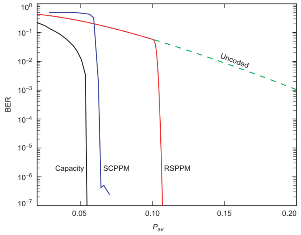
Channel coding is a very important block in the transmission chain to ensure the reliability of DS communication. Typically, applying ideal error correction code (ECC) can lead to reaching the capacity limit, i.e, the maximum possible achievable capacity. However, such codes are hard to construct. Therefore, it is important to take into account the code efficiency when designing the communication links [51]. The code efficiency refers to the difference between the capacity limit and the error code threshold at a specific bit error rate (BER). The smaller the code efficiency, the closer the link capacity to the capacity limit is. As a reference, an uncoded system would have a code efficiency in the order of [48]. In the early missions to space in the sixties, a decision was needed on whether to rely on block codes or convolutional codes [52]. For marinar ’69, block codes where the best options at that time given sequential decoding implementation was not that efficient at that time. Such choice led to a poor data rate. Thanks to the efficient implementation of sequential decoding, convolutional decoding has been adopted starting from Pioneer 9. Such a change offered a better coding gain of compared a . Since then convolutional codes under different variants has been adopted for DS communication such as Turbo code [53]. Reed-Solomon codes are commonly used with convolutional codes for DS application as it is efficient in correcting complex and bursty errors [38, 46, 28, 54], and has a code efficiency in the order of to when its being used with PPM [55]. Nevertheless, the most recommended and efficient coding that can be used in DS systems is the serially concatenated pulse position modulation (SCPPM) [56, 57, 48]. This coding techniques has an efficiency between and [55, 48]. In Fig. (2.4), we show the bit error rate of SCPPM compared to the capacity limit, Reed-Solomon with PPM and uncoded PPM.
Recently, there has also been some suggested codes in the field. For example the authors in [58] show that coded optical wavelength division multiple access (WDMA) with PPM can be a good candidate for DS. Using the coding gain metric, which is the power gain over uncoded case, WDMA has a gain for a coding rate, and a coding gain for a coding rate of at a frame error rate (FER) of [58]. Since fixed-rate codes like LDPC and Turbo codes are not efficient for DS communication since it fails to adapt with the changes in DS communication link due to time variability, authors in [59] propose the use of rate-less codes (e.g. Raptor codes), and hence achieves a better performance than LDPC and Turbo codes. The authors propose to further combine between spinal and polar coding to achieve even better performance.
The reliability of DS link is explored by a number of other techniques in addition to the coding. We next address the important aspects of DS networking protocols and some related challenges.
2.3.3 Detection
Advances in detection technology play a role in providing efficient DS communication. A detection method can either be coherent or non-coherent. Coherent receivers, for example heterodyen and homodyne, have a higher spectral and dimensional efficiency, which is the capacity to use different modes (degree of freedom). However, they suffer from limited photon efficiency, but tend to be more practical when very high data rates are required. Non-coherent receivers, on the other hand, are energy efficient, but that comes at a cost of exponentially decreasing dimensional efficiency [60].
Rendering to their energy efficiency, non-coherent receivers are commonly used in DS such as Direct detector [55, 61]. There are different types of direct detectors among which are APD, PIN which stands for p-type, intrinsic and n-type semiconductor regions in the diode structure, and PC.
Due to their high photon efficiency comparing to other conventional direct detection methods, PC detectors are getting a great attention and recommended, along with PPM modulation, to be used in the future DSOC. These detectors are able to count a single photon incident on them.
It can be viewed as an extension of APD detectors with infinite gain in which a digital output signal is generated for each detected photon [61]. They can offer up to gain over APD [28].
However, PC detectors faces many challenges.
Typically, signals incident on DSOC detectors are faint, not only because of the huge distances and associated losses, but also due to constraints on spacecraft power and laser electrical-to-optical conversion efficiency.
Therefore, to improve communication reliability detector sensitivity combined with high quantum efficiency at wavelengths of interest, are highly sought after. Here, PC efficiency is the probability that the detector generates an electron corresponding to the detected photon.
Furthermore, DS optical links are rendered viable by reducing the duty cycle of the laser transmitter so that the power peak of the laser pulse can overcome the huge space loss, as well as associated system and channel losses, so that a few signal photons arrive at the detector. This calls for temporally narrow pulses, typically in the order of few long [27].
The noise sources that affect PC detection process are the background noise, which comes from diffused energy from the sky, planets, or stars in the field of view of the receiver, dark counts electrons generated by the photon detectors, and thermal noise of the receiver [27]. In addition to the noise, receivers implementing PC detection schemes suffer from the following two losses
- •
Blocking loss. Due to the binary nature of the detection output, noise in the detection process appears in the form of dark counts or varying detection efficiency. As a result, the detector gets blind after a detection event missing all incident photons until reset, leading to a blocking loss. Hence, the detector is limited to counting at most one photon per reset time or dead time [62].
- •
Jitter loss. The random delay from the incident of a photon on a detector to the time an electrical output pulse is generated in response to that photon [63] is called a jitter loss. A significant loss occurs if the standard deviation of the jitter is in the order of the slot width of the pulse.
PPM-PC technologies have been demonstrated by NASA to achieve data rates of several hundred megabit per second, e.g. with a PPB sensitivity in the Lunar Laser Communication Demonstration and with a sensitivity of detected PPB [49].
We provide next examples of PC detectors that can be used for DS applications.
- 1.
The intensified photo diode that uses wavelengths of and with minimum slot widths of approximately , and supports data rate.
- 2.
- 3.
Superconducting nanowire single photon detectors [66].
2.4 Space protocols
In addition to the different physical layers techniques such as modulation, coding and detection, network protocols are of paramount importance to make the communication links reliable and overcome the different complex challenges. Hence, seamless connection and coordination between satellites, ground communication systems on Earth and DS probes at the final terminals are needed. In such complex and challenging environment, due to losses, extreme distances and space characteristics, matured terrestrial networks protocols are of no use, hence calling for well tailored network protocols, called DS internetworking [67].
In this perspective, NASA for example relies on delay/disruption tolerant networking (DTN) as an intuitive solution for space missions since these networks can handle excessive delays and fast changing environment, and yet maintain reliability. To coordinate the networking efforts between the different space agencies, consultative committee for space data systems (CCSDS) has been working on different protocols and architectures such as SCPS architecture [68], space packet protocol architecture [69], several internet protocols, and especially the DTN architecture [70, 71, 72].
With early missions to space, point to point or single relay links was possible especially link to low-Earth orbit. However, with missions to deeper space, DTN architecture, thanks to the automatic store-and-forward feature, becomes a natural choice due to its ability in handling long and variable delays, and link intermittent connectivity issues [73]. Automatic store-and-forward mechanism not only allows to forward packets to next destination, but also to keep a copy for future use if packet was not successfully delivered [74].
Current and future internetworking protocols have many challenges to overcome such as network topology dynamicity, links and entity heterogeneity, DTN scalability and also the ability to support possible future services. Some of these concerns have already been raised such as the need for future services such as broadcast, multicast and streaming [75].

2.4.1 Discussions and outlook
In this section, we discussed the potential modulation and coding schemes for DS communication. It is worth reiterating that yet experimentation of the efficiency of existing schemes needs to be conducted for DSOC. The selection of the PPM order needs to be thoroughly studied and carried based not solely on the achieved capacity but rather on other criteria such as BER, transmitter and receiver complexities, link gains, etc. Similar studies are needed from coding perspective to explore the possibility of new codes developed for DS communication. DS systems are expected to operate at speed of several tens of gigabits per second and beyond and hence will require a major improvement over existing receiver technology both in terms of data rate and sensitivity. Even though coherent receivers can in principal provide near-quantum-limited receiver sensitivity, such a performance is achieved by strict conditions, which make direct detection receivers simpler to achieve and in general provide better performance [46].
As a result, in addition to their energy efficiency and simplicity, non-coherent detectors are preferred over their counterpart. Nevertheless, coherent detection has recently started to get more interest due to their ability to increase the capacity in DS communication [49].
Based on [76], while using a single-quadrature homodyne receiver (without a pre-amplifier) resulted in a sensitivity of at , demonstration with erbium-doped fibre amplifier coherent receivers that is pre-amplified results in with only PPB increase in sensitivity [77, 78].
At the network protocol level,however, there is a need for advanced DTN protocols tailored for DS links accounting for the high delays and intermittent losses.
2.5 Capacity limit
In order to decide on the modulation, coding, and detection strategies, channel capacity needs to be quantified. The Shannon capacity gives the the maximum rate in a communication channel in classical information theory [79]. In the context of DSOC, the capacity is characterized by Holevo information which is based on quantum mechanic theory. The analytical closed form expression of the quantum capacity is derived based on Holevo theorem [60], which is, asymptotically, formulated as where is exponential constant, is the dimensional efficiency expressed as mode/bit and is information efficiency in photon/bit unit. In theory optimal coherent-state modulation achieves the ultimate quantum limit but practical sub-optimal coherent receivers are operating in near limit but in the low photon efficiency region as they hit a birck wall of 1.44 bits/photon and by that are not efficient for DS application [60].
In the case of PPM-PC receivers, the capacity can be approximated with respect to Holevo limit as follows [60, 80].
| (2.8) |
proposes using coherent states with PC to get closer to Holevo limt as its easy to produce coherent states but it challenging and very impractical. Instead, suggests using quantum number state (NS) communication, where number state is a quantum state well-defined number of photons, with the fact that quantum states are hard to produce, NS is more practical then the former method and could reach to the Holevo limit [81]. Nonetheless, achieving so requires very high channel transmittivity which means the probability of transmitted NS photon is received at detector. We can see from the following formula how NS communication effected by transmittivity of the channel which is , where is multiplicative factor, in the case of OOK where and when , . but for PPM . As shown in Fig. (2.6) hence, PPM will not reach the holevo limit, even when . With a transmittivity of one, NS along with OOK gets to the ultimate limit. In Fig. (2.6), in addition to Holevo limit, we show the capacity limit for PPM plus PC and quantum number state modulation with OOK and PPM. The figure demonstrates how as quantum number state transmittivity () gets higher, the capacity gets closer to the Holevo limit in the case of OOK.
| Average | Planet | Received | Reached | Average |
|---|---|---|---|---|
| Distance | power | capacity | delay | |
| (Km) | (W) | (Mbps) | (Minutes) | |
| 58 million | Mercury | 5.1856e-6 | 139.45 | 3.22 |
| 225 million | Mars | 4.5053e-6 | 123.42 | 12.5 |
| 778 million | Jupiter | 1.7741e-6 | 52.527 | 43.22 |
| 1.2 billion | Saturn | 9.2772e-7 | 28.173 | 66.66 |
| 4.5 billion | Neptune | 7.8951e-8 | 2.4598 | 250(4h) |
| 5.9 billion | Pluto | 4.6219e-8 | 1.4409 | 327.77(5.46h) |
In Table 2.1, we show the achieved soft capacity which is based on the probability as a result of counting incoming incident photon that indicate if there is a pulse or not [81]. For one PPM-PC detector at the average distance of various planets. We assume the transmitter and receiver diameters to be and respectively, transmitted power, time slot, modulation order 16, and noise power reaches to . And path loss for example for the average distance of Mars is , the sum of other loss for the received power not including the detection loss is , and the detection loss is .
Noticing how the capacity dramatically gets smaller as we get to a further planet distances. Things gets even worse as the planets get further far from the Earth.
3 DS Communication Advances
3.1 Orbital Angular Momentum
To better utilize the tremendous capacity offered by FSO, a great deal of attention is being giving for exploring the potentials of merging the FSO with OAM which emerges as a technology to solve the high date rate demand of future near-Earth and DS communications. Thanks to the fact that the helical wavefront of a photon is distributed in infinite ways (or modes) spatially, allowing waves with various phase fronts to be multiplexed and transmitted over the same frequency spectrum since they can be distinguished after they propagate in space. Next, we show the mathematical representation of OAM modes.

The mathematical description of the electromagnetic wave in the cylindrical coordinate is expressed as the laguerre-gaussian beam (LGB) given by [83] as:
| (3.1) |
Where r, and z are cylindrical coordinates, is the azimuthal phase profile taking a value from 0 to 2. is the azimuthal index specifies the mode which translates to the number of twists per wavelength. The sign of the mode (positive or negative) represents the direction of twist (clock or counter clockwise respectively), is the radial mode index which indicates the polarization of the beam. , where is the beam waist at , is the Rayleigh range which is the distance where the cross section of the beam is doubled. is the radius of the beam at . is the associated Laguerre polynomial, is a normalization constant, and is the Guoy phase shift which is axial shift that a converging light wave experiences as it passes through its focus, where n is a dimension that equals 1 in case of cylindrical wave and equals 2 when the wave is spherical [84].
The generation of OAM beams could be done using spiral phase plate (SPP) which is a crystal plate that has a helical shape structure converts Gaussian beams to OAM. Moreover, diffractive phase holograms, metamaterials, cylindrical lens pairs, fiber gratings, and couplers each of which can generate OAM beams. The q-plates also can convert the spin angular momentum (SAM) of light to OAM [85]. For more about generation methods see [86, 87].
Detection of OAM modes on the other hand can be achieved using either the inverse helical phase hologram, q-plates, SPP, photonic integrated circuit, free-space interferometers, which an instrument for measuring optical properties, or mode sorter which is capable of demultiplexing multiple of orthogonal spatial components occupying the same space [88].
Specific arrangements in the generation side results into different beam types. such as Mathieu, Bessel, Ince-Gaussian, vortex, hypergeometric, and laguerre-gaussian beam (LGB) s each of which has different characteristics. Perfect vortex beams could perform better then laguerre-gaussian beam (LGB) s under turbulence based on quantum communication system [89]. Bessel beams, on the other hand, are diffraction free and have superior self-healing capabilities (size preserving for example) hence have resiliency against AT but only for very limited distances [90, 91, 92]. Comparing to Bessel beams, however, laguerre-gaussian beam (LGB) s can, due to their self-healing property, propagate farther distances and hence more roubst [93]. laguerre-gaussian beam (LGB) s are the most applied type in DSOC [93].
3.1.1 Challenges
Many recent research and experimental works have, unprecedented, exhibited very significant results in the possibility of establishing several terabit per second capacity for OAM-based communications [37, 94]. OAM does not only tremendously enhance the spectral efficiency, it also offers a great deal of improvement for two other very important aspects of communications, namely energy and security [95, 96].
Nevertheless, there are some major challenges, listed below, facing DSOC OAM implementation. For the best of our knowledge, thoroughly discussions of OAM DSOC challenges and some proposed mitigation are being presented for the first time.
- 1.
Atmospheric turbulence. OAM modes are very vulnerable to AT, as it leads to crosstalk which render the orthogonality between OAM states to be no longer preserved. Even though, AT is not of a concern in space-to-space link [29], it is the main challenge of OAM-DSOC probe-to-Earth links.
- 2.
Spatial spread. The LGB intensity profile exhibits a donut style that gets bigger, i.e. spreads more spatially or diverge, as the beam singularity increases. The good news is that it has be proven experimentally that OAM signals or modes, even though diverge, preserve their orthogonality and hence can be detected even if the LGB is only partially received [97]. More specifically, even if a quarter or multiple of a quarter of the donut-profiled beam is captured by the receiver, OAM signals can still be recovered. Considering the DS distances, we, in Fig. (3.2(a)) (a) and (b), show the dimensions (in terms of profile diameter) and spatial intensity profile of the LGB. The dimensions and spatial distribution are provided at the farthest distance Earth-to-Mars, namely for ,. As we can notice, the Gaussian beam () dimension is smaller than that of the OAM-LGBs. Moreover, the beams diverge more as their modes increase. In Fig. (3.2(a)), is the dimension of OAM beams sent from Earth to Mars with transmitter diameter of 1m, as shown it diverse more the higher the mode number selected. In Fig. (3.2(b)), the OAM beams preserve its shape in very long distances as an indication to where to place the receiver in such long distances between the transmitter and receiver as the there is a singularity in the middle of the beam wave front, and if partial detection in this range is accomplished [98].
- 3.
Lateral displacement error. Keeping the LGB axis and the receiving end fully aligned is difficult for an actual communication system. For long distance transmissions, this requirement is even stringent. Alignment error does not only render optical power loss, but also, more crucially, causes expansion of the spiral spectrum and thus crosstalk effect and mode detection difficulty [99]. In fact, however, it has been shown that the later offset may improve resiliency against eavesdropping [100].
3.1.2 Mitigation
We, in Table 3.1, highlight OAM sate of art that address the OAM achievable capacity, detection in presence of AT, and partial beams reception. Although there are significant contributions addressing the FSO-OAM challenges, however they are mostly limited to few kilometers distances. The OAM detection challenges in presence of divergence issue and the possibility of recovering modes from a small fraction of the OAM beam traveled DS distances, however even though imperative in the OAM technology implementation, it is still an open research problem. Aside from [101, 102], there are no other references that analyzed OAM challenges in DS.


| References/Year | Model | Distance | Results |
|---|---|---|---|
| Area: capacity improvement | |||
| [103](2012) | 16QAM polarization multiplexed with 16OAM modes and | 1m | Capacity of 2.56 Tbit/s and spectral efficiency of 95.6bit/ s/ Hz |
| [102](2011) | For deep space and near-Earth communication with LDPC-coded OAM modulation and multiplexing as a additional degree of freedom. | The spectral efficiency of proposed scheme is times better then PPM, where N is the number of OAM modes used. | |
| Turbulence compensation | |||
| [106](2020) | Adaptive optics compensation approach based on the wirtinger flow (WF) algorithm. | 1km | The RMS error reduces to compared with for the conventional gerchberg-saxton algorithm |
| [107](2020) | Using gerchberg-saxton (GS) algorithm and convolutional neural network | 1Km to 6Km | Recognition accuracy of in high turbulence strength of 69.50 To 100 for medium and weak turbulence levels |
| [108](2020) | Sensorless adaptive optics (AO) and a convolutional neural network (CNN) to demodulate OAM modes | 1.2Km | BERs under strong turbulence decrease from to |
| [109](2020) | Convolutional neural network (CNN), a deep learning (DL) technique | 1Km to 6Km | Recognition accuracy of 97.1 under moderate turbulence and 80 under strong turbulence |
| [110](2019) | Diffractive deep neural network (D2NN) 10 types of multiplexed OAM modes. | Recognition accuracy in high turbulence strength of 50 To 100 for medium and weak turbulence levels | |
| Partial reception | |||
| [97](2013) | Using IR camera with SLM and a technique transform OAM states into transverse momentum states | 4km | Capacity of 200Gbit/s |
| [111](2018) | System modal for detecting a reduced area receivers | 1 km | 12 b/s/Hz higher rate at SNR 25dB then using a complete are receivers |
| [112](2019) | Using synthetic partial aperture receiving (SPAR) approach | Adjacent modes crosstalk could reach to 22, for non-adjacent modes crosstalk could reach as low as 7.71 | |
The authors in [102] proposed combining the LDPC code with OAM-based modulation schemes to overcome AT effects. With their presented methods, the authors in [102] achieved a spectral efficiency of over that of PPM modulation, where is the modulation order and is number of OAM modes.
Mode Modulation we suggest a simple yet promising idea,which apparently turned out to be also suggested by [113] which we refer to as mode modulation (MM), to overcome crosstalk, increase power efficiency, and spectral efficiency. In MM, we propose instead of multiplexing mode and having to handle the crosstalk and the degradation cause in performance and limitations it causes in transmission distances, we send only one mode at a given signaling time.
In addition to the information carried by an OAM mode, we use the mode number to carry some information (and hence the name mode modulation). Without loss of generality, let where is integer. We can map each possible bit sequence to a unique mode number and hence extra information
can be carried by each mode. For example,
if we use two modes (represented by bit zero) and (represented by bit one) to transmit a sequence of binary bits we only need to transmit one bit over the mode specified by the consecutive bit. Example to send the sequence we only send bit zero over mode and bit 1 over mode . In this case, we have doubled the capacity without the burden of dealing with crosstalk and cost of the power consumption. More general, MM increases spectral efficiency by . To detect the signal correctly at the receiver side, however, the mode needs to be detected as well as the data carried by the mode. In our future work we propose to analyze the performance of the MM modulation analytically and experimentally.

3.2 Interplanetary Network
NASA has three operational networks that provide communication services to supported missions: DS network, near Earth network, and space network. DS network consists in multiple antennas distributed around the world. On the other hand, near-Earth-network consists of ground stations that provide communication and tracking services. The space network (SN) is a constellation of geosynchronous relays which consists of 10 satellites, called tracking and data relay satellite system (TDRSS) [75]. Connecting these networks with the relay system distributed around space is the first step to make interplanetary network (IPN).
In Fig 3.4, we illustrate current RF-based and future optical interplanetary network. In 2016, NASA lunched Next-Generation Space Relay Architecture Concept Study for 2040 to evolve NASA’s space communication and navigation networks. Planetary relays such as Mars relay is expected to operate using RF bands, mainly Ka and X bands, providing up to 125 Mbps and also optical links that provide up to 300 Mbps.
Potential solutions have been proposed to be implemented in the near to long term for IPN with different techniques. These ideas include optical communication terminals on planets that provide data rate to times higher than RF [114]. Also, other solution includes locating spacecrafts with respect to Sun-Earth’s Lagrangian points to overcome obstruction or conjunction in the way of the links. However, the most interesting idea is implementing IPN with thousands of what is known as cube-sats, which are small satellites promising high speed using optical communication. These cubesats are distributed in the space promising achievable rate of 2Gbps [115, 116].
3.3 Quantum Communications
Some of the quantum properties had gain attention to be used in communication network by using the quantum states to carry information [117] . A quantum communication (QC) is expected to break through the limit of classical communication technology in the aspects of communication security, computing power, information transmission [117]. However, what is unique about QC is that theatrically quantum cryptography promises to obtain absolute secure channel. There are many techniques in QC among which are quantum key distribution quantum key distribution (QKD), quantum teleportation (QT), quantum secret sharing (QSS), quantum secure direct communication (QSDC) and many more. QKD is one of used protocols in free space communication as well as fiber optics that has been proven it can achieve an average secret-key rate of Kbits for up to Km distance [118]. However, a global QKD and similarly sclable QC are not been realized yet mainly due to the fact that quantum repeaters [119, 120] can not be deployed [121]. Hopefully with ongoing research in the field, teleportation between photons without classical link restriction, distributed in the interplanetary network would be possible and hence alleviate the latency resulting from the long distances in communication links.
4 DSOC Link Engineering and Performance Analysis
In this chapter we first discuss the design link parameters for PC-PM detector and conclude their values for a desired data rate, then we get a closer look on performance analysis of the link at different characteristics.
4.1 Link Design for PC-PPM Based on Required Performance
Link design for DS communication in general has specific concerns. Depending on the distance, mission requirements, capacity needed, atmospheric conditions, Sun-Earth-probe angle and Sun-probe-Earth angle, modulation and coding used through out the mission can be adapted to get the best performance out of the link. The capacity of the communication link is a function of the received and noise power, modulation type, coding scheme, and the detection method which in this analysis would be photon-counting. PPM operates efficiently at high peak to average power ratio, hence it is suited for DS environment. In this section, the method for selecting the PPM order and coding to achieve a certain data rate is described. The modal of the channel used is Poisson, which is commonly adopted for DS optical links. According to the quality of service (data rate in this context) that needs to be met, the required power is concluded. The error correcting codes, are also chosen based on the targeted data rate. The good candidate coding algorithms for DS communication are the RS and SCPPM. Since the later out preforms RS, as stated in chapter 2. SCPPM is chosen in this design process (similar to [62, 27]). Depending on information provided to the decoder by the receiver, capacity can be categorized either as hard or soft [46]. In one hand, in case the receiver estimates each PPM symbol, the resulted capacity is referred to as hard capacity. This capacity is specified based on probability of symbol errors. However, if the receiver makes a decision based on counting photon per slot, the capacity is categorized as a soft capacity. This capacity as at least as high as as the hard as counting slot provide more information to the decoder.
Our analysis through out the chapter is based on soft capacity in a possion modeled channel using direct detection photo-counting detectors [61]. The following equation is Eq. (2.2), approximated soft capacity of poisson channel, which we explained previously to give overall idea about achievable DS link capacity, as it will be used for the DS link analysis and included in producing the graphs.
In Fig. (4.1) we plot the capacity against power received for different PPM order. For low power regime, the highest capacity is achieved by the highest order (i.e. with the modulation scheme corresponds to the slowest data rate). As the power increases, however, lower order schemes would be efficient to get a higher capacity Fig. (4.1).
In Fig. (4.2), the impact of noise on the achievable capacity at different received power is shown. As depicted in this figure in the case of , when power received reaches , noise will start not to have an effect on capacity. In other words, at some range of noise power, there is a threshold of required power that gives the maximum capacity for a given order and noise in that range will not have an effect.
It is worth mentioning that, for Mars links the is in the range to depending on the receiver used [27].
4.1.1 Parameters selection
Operation close to capacity is achieved by selecting the optimum PPM order for the desired rate. In addition to order selection, concatenating the PPM with an ECC so that the decoded BER satisfies some threshold is crucial. The optimal order and ECC rate vary with and . While is the average number of single photons per pulse, is average number of noise photons per slot time. is given by to , Where is the average number of single photons incident on the detector per second, and is the quantum efficiency of the detector which will be discussed in the next section of performance analysis. is given by , where is the average number of noise photons incident per second. To optimize the throughput over the course of a mission may require an adaptive choice of a set of modulation orders and corresponding ECC s [46, 62].
4.1.1.1 Modulation order
Choosing the optimum modulation order, denoted by , may depend on many aspects. Maximizing capacity for a given received and noise power is an important factor for design and hence the choice of . The formula below [62].
| (4.1) |
Illustrated in Fig. (4.3), is optimum modulation for different values of . Switching to the maximum order that will get the desired capacity. increases with increasing , and Similarly decreases with .
4.1.1.2 Coding design
Choosing the error code ratio is a function of the desired capacity and modulation order at that capacity [62].
| (4.2) |
Where the capacity unit would be in Gbps.
4.1.1.3 Required power
In this section, we show how to make modulation and coding design based on a certain data rate requirement and hence determine the power needed to achieve the desired performance. Suppose a system with a slot width of and background noise and we are interested to find the power needed to achieve a rate of and choose appropriate coding and modulation parameters. From Fig. (4.1), we find the optimum PPM order to achieve this data rate is , and the minimum required power is which can be represented in single photon per slot which is equals to , going back to Fig. (2.4) in chapter 2 . To achieve 56 Mbps, we choose a rate following Eq. (4.2), ECC and concatenate it with 64-PPM. The performance of two candidate ECCs for this operating point are SCPPM(, , , ) and RSPPM(, , ) are illustrated in Fig. (2.4) in chapter 2. Their performance may be compared with capacity for and the uncoded performance, which, since it carries no coding redundancy, yields . The SCPPM code operates & from capacity, the RS code operates from capacity, and uncoded PPM from capacity (at 56 Mbps). An appropriate comparison for uncoded -PPM is with capacity for , from which uncoded performance is . (It would be more efficient to achieve with a rate code mapped to -PPM).
4.2 Link Performance for Given Parameters
The values used trough out this section are based on consultative committee for space data systems (CCSDS) [122], for high photon efficiency (HPE), with the assumption of cloud free line of sight (CFLOS) and the DS channel represented as a Poisson channel. Due to the limited power nature of the link, intensity modulation (IM) and direct detection (DD) with photon-counting detectors are considered for receiver architecture. Under these conditions, the PPM signaling and a serially concatenated pulse position modulation (SCPPM) error code is used [62].
Through out this section, we, unlike the previous one, for a given set of parameters (that may or may not be set based on CCSDS) tend to evaluate the DS link performance.
4.2.1 Received power – before the photon detector:
The received power after the receiver telescope and before the photon detector Pr,ap (Watt) can be estimated as:
| (4.3) |
Where is the transmitted power, as defined previously, and are the transmitter and ground receiver aperture gains, respectively. is the free space loss factor, is the atmospheric transmittance, is the cirrus transmittance factor, is the scintillation loss factor is the pointing loss factor, ŋt and ŋr are the transmitter and receiver efficiencies respectively. These parameters are to discussed below.
4.2.1.1 Free space loss
Free space loss due to the optical wave propagation from the transmitter to the receiver is defined as follows, where is the wavelength and distance is in meters.
| (4.4) |
4.2.1.2 Transmitter and receiver gain
The transmitter gain can be estimated using the following formula, with the diameter of the transmitter aperture of the telescope:
| (4.5) |
The equation before simplifications is , where in rad is half beamwidth angle and equals to , and if the beam is Gaussian , which its the case in this analysis, so the gain would be Eq. (4.5). The majority of receiver telescopes used in optical communications have central obstruction such as the secondary mirror of Cassegrain telescopes, to increase focal length which in return decrease the transmitted optical power and make the beam narrower. This type of telescopes consists of two mirrors, a primary and a secondary. The primary mirror has larger diameter than the secondary one, while the secondary obscures the primary [123, 124]. Receiver gain is as follows:
| (4.6) |
Where is the receiver’s primary aperture diameter in meters, r is the receiver’s obscuration ratio which is . br is the receiver’s secondary aperture diameter.
4.2.1.3 Atmospheric transmittance
4.2.1.4 Cirrus transmittance
CFLOS transmission is assumed. However, even when the sky appears relatively clear, semi-transparent ice clouds, cirrus clouds, can be present along the path, however, in DS analysis cirrus clouds losses are accounted for by taking an additional power margin [126].
4.2.1.5 Scintillation loss factor
4.2.1.6 Pointing error loss factor
The necessity for narrow beam width subject to the long range of a DS link makes accurate pointing critical. Pointing losses may arise due to the jitter and pointing bias. Pointing error loss can be estimated for a specific probability level, from the probability density function of normalized received intensity taking into account the pointing error. A pointing error of radians, where and are the signal wave length and the transmitter diameter respectively corresponds to approximately intensity reduction [55, 123].
| (4.7) |
Where is the total variance of pointing errors.
4.2.1.7 Transmitter/receiver efficiencies
The transmitter/receiver optical efficiencies are introduced as a way to capture the losses due to the coupling of the laser beam to the optical system. Transmitter/receiver losses are denoted by / [62].
4.2.2 Detected power
Detected power, for photon-counting detector are effected by blocking loss and jitter losses and also the detector’s quantum efficiency, , which states the probability of the photon that will generate a corresponding electron.
| (4.8) |
4.2.2.1 Detector blocking loss
photon-counting detectors become inactive (blocked) for some time after the detection event, as we discussed in chapter 2. This blocking leads to losses relative to an ideal detector, based on Markov model for the detector state [130]. Assuming high signal to noise ratio (SNR), blocking loss for single detector which is in this case is equal to:
| (4.9) |
and are the noise and signal photon flux (photons/s) on the detector respectively. , , and denotes the dead time in seconds, i.e., the duration of blocking. is the noise power and is the energy per photon (). is the Planck’s constant, is the speed of light, and is the wavelength. in Fig. (4.4), and in Fig. (4.4(a)), for distances of and Fig. (4.4(b)), for closest to the furthest distance to Mars. As shown as gets further away, blocking loss gets lower, because the number of photon that are received is low.
4.2.2.2 Detector jitter loss
In photon-counting detectors, there will be a random delay from the time a photon is incident on the detector to the time an electrical output pulse is generated in response. That random delay, called detector jitter, produces losses since the signaling depends on identifying the pulse position in time analytical expressions for the computation of jitter loss as a function of the normalized jitter variance.
| (4.10) |
| (4.11) |
Where is the coding ratio, is jitter detector loss and is the standard deviation of jitter. As shown for less then jitter loss is negligible but when the ratio is higher then , the losses are sufficiently large, as to typically make the operating point prohibitive [63].
4.2.3 Required power and coding efficiency
The required power at the receiver is expressed in terms of coding efficiency and detected power as follows.
| (4.12) |
Where denotes the coding implementation loss and the coding efficiency, the gap to the theoretical capacity. In practice codes only approach the ideal performance. Therefore, code efficiency is the extra power is needed in order to achieve the ideal performance for a specified BER [48].
4.2.3.1 Noise contribution
Because of the photon detection nature some noise sources are accounted, e.g., the background noise, dark counts, and leakage power from the transmitter. The total detected noise power is described as follows [61]:
| (4.13) |
By working on only one detector , , measured in electrons per seconds per meter squared, is each detector’s dark rate. is the leakage ratio. , measured in Watt, is the background power (to be discussed in more details) per detector, and is the diameter of each detector.
4.2.3.2 Background noise
The power of the background signal at each detector comes from the energy diffused from the sky, planets, or stars which are in the field of view of the receiver :
| (4.14) |
Here is the field of view of the receiver’s aperture in steradian (Sr). is expresses based on [51, 131] as follows
| (4.15) |
Where (m) is the focal length of the telescope. is receiver area in (), and is the efficiency of the receiver. is the background radiance energy density of large angular sources (i.e., planets, sky) and the stray light that scatters into the detector’s field of view. changes in different situations for example if it is a terrestrial station on Earth it can get to at a sunny day and at night is . is the irradiance energy density of point sources that it might get in the field of view (i.e., stars), which depend on the wavelength, with that atmospheric losses are also included [132]. is the receive bandpass optical filter width in millimeter (mm).
4.2.4 Numerical analysis for Mars and beyond communication links
To show how to do some performance analysis, we in the Table.(4.1) we provide some values of the system parameters explained through out the previous sections.
The impact of different parameters on the capacity versus distance is discussed for the set parameters. We set different receiver diameter sizes then, modulation order, , and vary link distance to make it cover for the change in Earth-to-Mars distances ( to ) as well as for links at to distance form Earth. almost all of the values in the table obtained from [27].
| Wavelength (nm) | 1550 |
| Rang (AU) | 0.36/2.68 |
| Elevation angle (deg) | 20 |
| Transmit power (W) | 4 |
| Transmitter diameter (m) | 0.22 |
| Transmitter secondary diameter | 0 |
| Transmitter efficiency | 0.6 |
| Receiver diameter (m) | 4/6/8/10 |
| Receiver secondary aperture (m) | 0 |
| Receiver efficiency | 0.4 |
| Receiver quantum efficiency | 0.5 |
| Focal length of the receiver (m) | 16 |
| Detector diameter (m) | 30e-6 |
| Optical filter (µm) | 0.2e-3 |
| Atmospheric efficiency (vertical) | 0.98 |
| Link margin (dB) | 4.0 |
| Pointing RMS error value (µrad) | 0.7 |
| Probability level | 1e-14 |
| Modulation | M-PPM |
| Modulation numbers | 16/64/256/1024 |
| Slot Time (ns) | 2/0.25 |
| Coding ratio | 0.5 |
| Background noise reduction | 0.5 |
| Coding efficiency | 0.8 |
| Radiance of planets + sky (W//Sr/µm) | 85 |
| Leakage ratio | 0 |
| Detector array | 1 |
| Detector dark rate (e/s/) | (1e+12) |
| Blocking time (ns) | 50 |
| Jitter time (ns) | 240 |
| Atmospheric transmittance | 0.943 |
| Scintillation loss (dB) | 0.01 |
| Pointing loss (dB) | 1.95 |
| Cirrus loss (dB) | 0.5 |
The result obtained in Fig. (4.6), calculated capacity at and shows that the bigger receiver diameter, the higher capacity is achieved also in the range of Mars distances it seems that the slop for diameters of is significantly higher then .
In Fig. (4.7), calculating the capacity for and but one for M= 16 and another at M = 256 and as shown for M=16 gives higher capacity then M = 256 in this rang of distances.
In Fig. (4.8), calculating the capacity for , M= 16, and both = 2ns and = 0.25ns. The lower the higher the capacity for the given range of distances, as the figure explains.
In Fig. (4.9) and . (4.10), is shown that gives the best capacity possible for the link for and , but for the later is shown that the capacity line has lower slop along Mars distances which indicates that bigger receiver diameters gives more satiable capacity along the Mars distance.
As going further away for Mars distances, we get from to from Earth does the response be the same?, Calculating the capacity for different M orders in this range of distances and the response shown in Fig. (4.11), in the case of and Fig. (4.12), for .
Fig. (4.9) and Fig. (4.11) we show achieved capacity of PPM system versus Mars and beyond Mars distances respectively, antenna diameter for transmitter and receiver are and respectively. The figure indicates how crucial the increase in DS communication distance is in determining the PPM system parameters and hence performance. As the modulation order decreases, the capacity of a given system improves by a significant margin until a certain distance. However as communication path takes a longer distance (in our settings close to ), the trend is the opposite. That is intuitive as increasing modulation order implies a reduction in the transmission rate and bit error rate (BER) as a consequence which becomes more crucial as distances increase (which results in a decreasing in the received power). In other words, the distance may impose us to increase the modulation order and hence the transmission rate to improve the system performance and maintain the highest capacity possible for a given channel model, detector, and other system parameters like receiver antenna diameter, and transmission power.
In the case of in Fig. (4.11), starting from roughly which is accomplished by , if is chosen, a capacity as high as is not used. As the distance gets further away at will get the highest capacity as it cross the line, and at an beyond gets the highest capacity. If there is not a switch to when it crosses and as it crosses , a capacity of is not utilized. For Fig. (4.12), beginning with for , if order or is chosen, capacity is not used. At cross and gives the highest capacity and takes over, and the different between the capacity for to again reaches to . in distance of gives the highest capacity of the link. Here if the link settled on one order along this range of distances, amount of capacity as big as is not utilized, this amount of data rate could be significant, which suggests using different Modulation number at different distances to Mars and beyond or along a missions.
4.2.5 CCSDS standard for selecting link parameters
After analysing performance of the link with different parameters values there is a methodology based on CCSDS aims at selecting parameters that maximize the data rate of the link and avoids tedious coded BER evaluations. Especially in case of a single photon detector or an array. It is mainly based on first considering all the combination of the link parameters which are the available PPM order, , coding ratio, and the computing the data rate with SCPPM coding for all the combination, and computing the received power by link analysis and the detected noise power, and then commuting the soft capacity of each power received calculated and noise power, based on that, selecting the best , , and that gives the highest data rate. Note that achieved data rate will be smaller than the capacity. However, if was free to take any value, then the capacity and the achieved data rate will be closer.
4.3 Discussion
Starting with how to select , , and the order for getting specific data rate and conclude the power required, seeing the behavior of PPM with different order verse power, the lower the power the higher order is respired for getting high capacity. Noise has some power threshold, if its passed, noise will not have an affect on the link performance. Getting more in details in the primary effects on the link which its major loss would be due to the long distance operation. Detection is effected with blocking and jitter loss, It would be low for low data rate operation, because not high number of photons are detected which is the case for DS communication. And further more, in numerical analysis as shown in Mars distances with the parameters used, is the dominated order to get the highest capacity. But that would change at different parameters values. For distances starting form to we got capacity in the range of for receiver’s diameter of , and for receiver’s diameter of , and a loss of if is chosen along the whole distance.
5 Conclusion
In this thesis, by performing link analysis in Mars distances using PPM, exploring FSO technologies in all network layers, and analyzing OAM propagation in DS, along with discussions on how to mitigate the advances’ challenges, we demonstrated the effectiveness and superiority of FSO compared to RF’s expected performance for DS communications. According to the PPM link analysis, the order of modulation that achieves the maximum capacity varies at different distances. We challenged the PPM scheme and the PC detection with other techniques for obtaining a higher capacity limit. We focused our attention on the key features and protocols of the DS network layers architecture and related possible enhancements that may lead to a interplanetary network. Further, we investigated how promising technologies would impact DS communications and pointed out the struggles and proposed solutions for accommodating OAM in DS environments which require further investigation.
References
- [1] International Space Exploration Coordination Group “Benefits stemming from space Exploration”, https://www.nasa.gov/sites/default/files/files/Benefits-Stemming-from-Space-Exploration-2013-TAGGED.pdf, 2013
- [2] National Aeronautics and Space Administration “NASA Perseveres Through Pandemic, Looks Ahead in 2021”, https://www.nasa.gov/feature/nasa-perseveres-through-pandemic-looks-ahead-in-2021, 2021
- [3] SpaceX “THE MOON: RETURNING HUMANS TO LUNAR MISSIONS”, https://www.spacex.com/human-spaceflight/moon, 2020
- [4] Bernard Edwards et al. “An update on the CCSDS optical communications working group” In 2017 IEEE International Conference on Space Optical Systems and Applications (ICSOS), 2017, pp. 1–9 IEEE
- [5] International Space Exploration Coordination Group “The Global Exploration Roadmap”, https://www.globalspaceexploration.org/wordpress/wp-content/isecg/GER_2018_small_mobile.pdf, 2018
- [6] China National Space Administration “Tianwen 1 makes orbital correction as Mars arrival draws near”, http://www.cnsa.gov.cn/english/n6465652/n6465653/c6811227/content.html, 2021
- [7] NASA “Mars 2020 mission Provenance rover” Accessed: 2021 URL: url{https://mars.nasa.gov/mars2020/spacecraft/rover/communications/}
- [8] European Agency “ExoMars 2022 rover”, https://www.esa.int/Science_Exploration/Human_and_Robotic_Exploration/Exploration/ExoMars/ExoMars_2022_rover
- [9] Richard Larsson et al. “Mars Micro-Satellite for Terahertz Remote Sensing” In EGU General Assembly Conference Abstracts, 2017, pp. 18645
- [10] Sissi Cao “Elon Musk Reveal’s SpaceX’s Timeline for Landing Humans On Mars” Accessed: 2020-02-12, https://observer.com/2020/12/elon-musk-says-spacex-will-land-humans-on-mars-in-a-few-years-if-theyre-lucky
- [11] European Space Agency “Exploring Mars”, https://www.esa.int/Science_Exploration/Human_and_Robotic_Exploration/Exploration/Mars
- [12] Antonios Seas et al. “Optical communications systems for NASA’s human space flight missions” In International Conference on Space Optics-ICSO 2018 11180, 2019, pp. 111800H International Society for OpticsPhotonics
- [13] Pantelis-Daniel Arapoglou et al. “Benchmarking the future of RF in space missions: From low earth orbit to deep space” In 2017 IEEE MTT-S International Microwave Symposium (IMS), 2017, pp. 388–390 IEEE
- [14] A. Kwok “DSN Telecommunications Link Design Handbook,206, Rev. B Telemetry General Information” Accessed: 10/31/2009 URL: url{https://deepspace.jpl.nasa.gov/dsndocs/810-005/206/206B.pdf}
- [15] “EMM Hope”, https://eoportal.org/web/eoportal/satellite-missions/content/-/article/emm-hope, 2021
- [16] NASA official website “Voyager” URL: url{https://voyager.jpl.nasa.gov/mission/science/}
- [17] Anatoly Zak “Robotic missions to Mars” Accessed: 2020-07-30, http://www.russianspaceweb.com/spacecraft_planetary_mars.html
- [18] The Society “Every Mission to Mars, Ever” Accessed: 2020, https://www.planetary.org/space-missions/every-mars-mission
- [19] “List of artificial objects on Mars” Accessed: 2021, https://en.wikipedia.org/wiki/List_of_artificial_objects_on_Mars
- [20] “List of artificial objects on Mars” Accessed: 2021, https://en.wikipedia.org/wiki/List_of_Mars_orbiters
- [21] Jet propulsion laboratory “Mars Reconnaissance Orbiter, Spacecraft Parts: Telecommunications” Accessed: 2021 URL: url{https://mars.nasa.gov/mro/mission/spacecraft/parts/telecommunicaverbtions/}
- [22] spaceflight101 “Spacecraft Information” Accessed: 2021-02-26, https://spaceflight101.com/maven/spacecraft-information/
- [23] “Viking 2 Lander”, https://nssdc.gsfc.nasa.gov/nmc/spacecraft/displayTelemetry.action?id=1975-083C, 2021
- [24] Jim Taylor et al. “Mars exploration rover telecommunications” In Deep Space Communications Wiley Online Library, 2016, pp. 251–356
- [25] “Mariner 4” Accessed: 2020 URL: url{https://nssdc.gsfc.nasa.gov/nmc/spacecraft/display.action?id=1verb964-077A}
- [26] “Viking 1 Orbiter”, https://nssdc.gsfc.nasa.gov/nmc/spacecraft/displayTelemetry.action?id=1975-075A, 2021
- [27] Nikolaos Lyras, Athanasios Panagopoulos and Pantelis-Daniel Arapoglou “Deep-Space Optical Communication Link Engineering: Sensitivity Analysis” In IEEE Aerospace and Electronic Systems Magazine 34.11 IEEE, 2019, pp. 8–19
- [28] Hamid Hemmati, Abhijit Biswas and Ivan Djordjevic “Deep-space optical communications: Future perspectives and applications” In Proceedings of the IEEE 99.11 IEEE, 2011, pp. 2020–2039
- [29] Hemani Kaushal and Georges Kaddoum “Optical communication in space: Challenges and mitigation techniques” In IEEE communications surveys & tutorials 19.1 IEEE, 2016, pp. 57–96
- [30] Karl Fielhauer, Bradley Boone and Daniel Raible “Concurrent system engineering and risk reduction for dual-band (RF/optical) spacecraft communications” In 2012 IEEE Aerospace Conference, 2012, pp. 1–7 IEEE
- [31] Matthew Grein et al. “An optical receiver for the Lunar Laser Communication Demonstration based on photon-counting superconducting nanowires” In Advanced Photon Counting Techniques IX 9492, 2015, pp. 949208 International Society for OpticsPhotonics
- [32] KE Wilson et al. “Results of the compensated earth-moon-earth retroreflector laser link (CEMERLL) experiment”, 1997
- [33] A Biswas, D Boroson and B Edwards “Mars laser communication demonstration: what it would have been” In Free-Space Laser Communication Technologies XVIII 6105, 2006, pp. 610502 International Society for OpticsPhotonics
- [34] RJ Cesarone, DS Abraham, S Shambayati and J Rush “Deep-space optical communications” In 2011 International Conference on Space Optical Systems and Applications (ICSOS), 2011, pp. 410–423 IEEE
- [35] David Oh et al. “Development of the psyche mission for NASA’s discovery program” In 35th International Electric Propulsion Conference, 2017, pp. 1–19
- [36] Abhijit Biswas, Meera Srinivasan, Sabino Piazzolla and Daniel Hoppe “Deep space optical communications” In Free-Space Laser Communication and Atmospheric Propagation XXX 10524, 2018, pp. 105240U International Society for OpticsPhotonics
- [37] Abderrahmen Trichili et al. “Communicating using spatial mode multiplexing: Potentials, challenges, and perspectives” In IEEE Communications Surveys & Tutorials 21.4 IEEE, 2019, pp. 3175–3203
- [38] Tomaso De, Enrico Paolini, Gianluigi Liva and Gian Calzolari “Reliability options for data communications in the future deep-space missions” In Proceedings of the IEEE 99.11 IEEE, 2011, pp. 2056–2074
- [39] Gengxin Zhang, Zhidong Xie, Dongming Bian and Qian Sun “A survey of deep space communications” In Journal of Electronics (China) 28.2 Springer, 2011, pp. 145
- [40] Weiren Wu et al. “Overview of deep space laser communication” In Science China Information Sciences 61.4 Springer, 2018, pp. 1–12
- [41] Mohammad Khalighi and Murat Uysal “Survey on free space optical communication: A communication theory perspective” In IEEE communications surveys and tutorials 16.4 IEEE, 2014, pp. 2231–2258
- [42] Donald Cornwell “NASA’s optical communications program for 2017 and beyond” In 2017 IEEE International Conference on Space Optical Systems and Applications (ICSOS), 2017, pp. 10–14 IEEE
- [43] Ibrahima Gueye et al. “Performance of Hybrid RF/FSO Cooperative Systems Based on Quasicyclic LDPC Codes and Space-Coupled LDPC Codes” In Wireless Communications and Mobile Computing 2020 Hindawi, 2020
- [44] Sky News “Mars: Three new space missions are about to reach the Red Planet - here’s what you need to know” Accessed: 2021 URL: url{https://news.sky.com/story/mars-three-new-space-missions-are-aboverbut-to-reach-the-red-planet-heres-what-you-need-to-know-12208547}
- [45] Joseph Statman and Charles Edwards “Coding, modulation, and relays for deep space communication Mars rovers case study” Pasadena, CA: Jet Propulsion Laboratory, National AeronauticsSpace …, 2004
- [46] Hamid Hemmati “Deep space optical communications” John Wiley & Sons, 2006
- [47] Jing Li et al. “Dual-pulse pulse position modulation (DPPM) for deep-space optical communications: Performance and practicality analysis” In 2012 International Conference on Wireless Communications and Signal Processing (WCSP), 2012, pp. 1–7 IEEE
- [48] B Moision and J Hamkins “Coded modulation for the deep-space optical channel: serially concatenated pulse-position modulation” In IPN Progress Report 42.161, 2005, pp. 1–26
- [49] Ravikiran Kakarla, Jochen Schr\"oder and Peter Andrekson “One photon-per-bit receiver using near-noiseless phase-sensitive amplification” In Light: Science & Applications 9.1 Nature Publishing Group, 2020, pp. 1–7
- [50] Robert Tyson “Adaptive optics and ground-to-space laser communications” In Applied optics 35.19 Optical Society of America, 1996, pp. 3640–3646
- [51] B. Moision, J. Wu and S. Shambayati “An optical communications link design tool for long-term mission planning for deep-space missions” In 2012 IEEE Aerospace Conference, 2012, pp. 1–12 DOI: 10.1109/AERO.2012.6187102
- [52] James Massey “Deep-space communications and coding: A marriage made in heaven” In Advanced Methods for Satellite and Deep Space Communications Springer, 1992, pp. 1–17
- [53] Dariush Divsalar and Fabrizio Pollara “Multiple turbo codes for deep-space communications” In TDA progress report 42.121 JPL, 1995, pp. 66–77
- [54] Robert McEliece and Laif Swanson “Reed-Solomon codes and the exploration of the solar system”, 1994
- [55] Hamid Hemmati “Near-earth laser communications” CRC press, 2020
- [56] Michael Cheng, Bruce Moision, Jon Hamkins and Michael Nakashima “SAT05-4: Implementation of a coded modulation for deep space optical communications” In IEEE Globecom 2006, 2006, pp. 1–5 IEEE
- [57] ITU-R SA.1742 “Technical and operational characteristics of interplanetary and deep-space systems operating in the space-to-Earth direction around 283 THz” In Geneva, Switzerland, 2006
- [58] Dariush Divsalar et al. “Wavelength division multiple access for deep space optical communications” In 2020 IEEE Aerospace Conference, 2020, pp. 1–13 IEEE
- [59] Hao Liang, Aijun Liu, Xinhai Tong and Chao Gong “Raptor-like Rateless Spinal Codes using Outer Systematic Polar Codes for Reliable Deep Space Communications” In IEEE INFOCOM 2020-IEEE Conference on Computer Communications Workshops (INFOCOM WKSHPS), 2020, pp. 1045–1050 IEEE
- [60] Sam Dolinar, Kevin Birnbaum, Baris Erkmen and Bruce Moision “On approaching the ultimate limits of photon-efficient and bandwidth-efficient optical communication” In 2011 International Conference on Space Optical Systems and Applications (ICSOS), 2011, pp. 269–278 IEEE
- [61] David Caplan “Laser communication transmitter and receiver design” In Free-Space Laser Communications Springer, 2007, pp. 109–246
- [62] B Moision and J Hamkins “Downlink Budget for Mars: Modulation and Coding” In The Interplanetary Network Progress Report, 2003, pp. 42–154
- [63] B. Moision and W. Farr “Communication Limits Due to Photon Detector Jitter” In IEEE Photonics Technology Letters 20.9, 2008, pp. 715–717 DOI: 10.1109/LPT.2008.919451
- [64] Jeffrey Stern and William Farr “Fabrication and characterization of superconducting NbN nanowire single photon detectors” In IEEE transactions on applied superconductivity 17.2 IEEE, 2007, pp. 306–309
- [65] Kristine Rosfjord et al. “Nanowire single-photon detector with an integrated optical cavity and anti-reflection coating” In Optics express 14.2 Optical Society of America, 2006, pp. 527–534
- [66] JPL “Superconducting Nanowire Single Photon Detectors for DSOC”, https://microdevices.jpl.nasa.gov/news/superconducting-nanowire-single-photon-detectors-for-dsoc/, 2021
- [67] Adrian Hooke “The interplanetary internet” In Communications of the ACM 44.9 ACM New York, NY, USA, 2001, pp. 38–40
- [68] Ian Akyildiz et al. “The state of the art in interplanetary internet” In IEEE Communications Magazine 42.7 IEEE, 2004, pp. 108–118
- [69] CCSDS 133.0-B-1 “Consultative Committee for Space Data Systems. Space packet protocol”, https://public.ccsds.org/Pubs/133x0b1c2.pdf, 2003
- [70] Scott Burleigh et al. “Delay-tolerant networking: an approach to interplanetary internet” In IEEE Communications Magazine 41.6 IEEE, 2003, pp. 128–136
- [71] CCSDS 714.0-B-2 “Consultative Committee for Space Data Systems. Space Communications Protocol Specification (SCPS)-Transport Protocol”, https://public.ccsds.org/pubs/714x0b2.pdf, 2006
- [72] Giorgos Papastergiou, Ioannis Alexiadis, Scott Burleigh and Vassilis Tsaoussidis “Delay tolerant payload conditioning protocol” In Computer Networks 59 Elsevier, 2014, pp. 244–263
- [73] Evan Jones and Paul Ward “Routing strategies for delay-tolerant networks” In Submitted to ACM Computer Communication Review (CCR) 1 Citeseer, 2006
- [74] Athanasios Vasilakos, Yan Zhang and Thrasyvoulos Spyropoulos “Delay tolerant networks: Protocols and applications” CRC press, 2016
- [75] Kanglian Zhao and Qinyu Zhang “Network protocol architectures for future deep-space internetworking” In Science China Information Sciences 61.4 Springer, 2018, pp. 1–16
- [76] ML Stevens et al. “Optical homodyne PSK demonstration of 1.5 photons per bit at 156 Mbps with rate- turbo coding” In Optics express 16.14 Optical Society of America, 2008, pp. 10412–10420
- [77] David Geisler et al. “Demonstration of 2.1 photon-per-bit sensitivity for BPSK at 9.94-Gb/s with rate- FEC” In 2013 Optical Fiber Communication Conference and Exposition and the National Fiber Optic Engineers Conference (OFC/NFOEC), 2013, pp. 1–3 IEEE
- [78] Domanic Lavery et al. “Realizing high sensitivity at 40 Gbit/s and 100 Gbit/s” In OFC/NFOEC, 2012, pp. 1–3 IEEE
- [79] Claude Shannon “Communication in the presence of noise” In Proceedings of the IRE 37.1 IEEE, 1949, pp. 10–21
- [80] Konrad Banaszek, Ludwig Kunz, Micha Jachura and Marcin Jarzyna “Quantum limits in optical communications” In Journal of Lightwave Technology 38.10 IEEE, 2020, pp. 2741–2754
- [81] Sam Dolinar, Bruce Moision and Baris Erkmen “Fundamentals of free-space optical communications” Pasadena, CA: Jet Propulsion Laboratory, National AeronauticsSpace …, 2012
- [82] “Orbital angular momentum of light”, https://en.wikipedia.org/wiki/Orbital_angular_momentum_of_light, 2021
- [83] Alonzo Espinoza et al. “Optical design of communication simulator for orbital angular momentum based free-space link with an adaptive optics receiver” In Laser Communication and Propagation through the Atmosphere and Oceans IV 9614, 2015, pp. 96140P International Society for OpticsPhotonics
- [84] Simin Feng and Herbert Winful “Physical origin of the Gouy phase shift” In Optics letters 26.8 Optical Society of America, 2001, pp. 485–487
- [85] Anita Thakur “Twisted light-propagation properties and particle dynamics”, 2013
- [86] Rui Chen et al. “Orbital angular momentum waves: generation, detection, and emerging applications” In IEEE Communications Surveys & Tutorials 22.2 IEEE, 2019, pp. 840–868
- [87] Kuang Zhang, Yuxiang Wang, Yueyi Yuan and Shah Burokur “A review of orbital angular momentum vortex beams generation: from traditional methods to metasurfaces” In Applied Sciences 10.3 Multidisciplinary Digital Publishing Institute, 2020, pp. 1015
- [88] Alan Willner et al. “Optical communications using orbital angular momentum beams” In Advances in Optics and Photonics 7.1 Optical Society of America, 2015, pp. 66–106
- [89] Ivan Djordjevic, Yequn Zhang and Xin Gao “Quantum channel capacity for OAM based free-space optical communications” In Quantum Communications and Quantum Imaging X 8518, 2012, pp. 851809 International Society for OpticsPhotonics
- [90] Christian Vetter et al. “Realization of Free-Space Long-Distance Self-Healing Bessel Beams” In Laser & Photonics Reviews 13.10 Wiley Online Library, 2019, pp. 1900103
- [91] Philip Birch, Iniabasi Ituen, Rupert Young and Chris Chatwin “Long-distance Bessel beam propagation through Kolmogorov turbulence” In JOSA A 32.11 Optical Society of America, 2015, pp. 2066–2073
- [92] Shuhui Li and Jian Wang “Adaptive free-space optical communications through turbulence using self-healing Bessel beams” In Scientific reports 7.1 Nature Publishing Group, 2017, pp. 1–8
- [93] Job Mendoza-Hern\’andez, Maximino Arroyo-Carrasco, Marcelo Iturbe-Castillo and Sabino Ch\’avez-Cerda “Laguerre–Gauss beams versus Bessel beams showdown: peer comparison” In Optics letters 40.16 Optical Society of America, 2015, pp. 3739–3742
- [94] Jian Wang et al. “Ultra-high 435-bit/s/Hz spectral efficiency using N-dimentional multiplexing and modulation link with pol-muxed 52 orbital angular momentum (OAM) modes carrying Nyquist 32-QAM signals” In 2015 European Conference on Optical Communication (ECOC), 2015, pp. 1–3 IEEE
- [95] Xiaole Sun and Ivan Djordjevic “Physical-layer security in orbital angular momentum multiplexing free-space optical communications” In IEEE Photonics Journal 8.1 IEEE, 2016, pp. 1–10
- [96] Ivan Djordjevic “Multidimensional OAM-based secure high-speed wireless communications” In IEEE Access 5 IEEE, 2017, pp. 16416–16428
- [97] Guodong Xie et al. “Analysis of aperture size for partially receiving and de-multiplexing 100-Gbit/s optical orbital angular momentum channels over free-space link” In 2013 IEEE Globecom Workshops (GC Wkshps), 2013, pp. 1116–1120 IEEE
- [98] Miles Padgett et al. “Divergence of an orbital-angular-momentum-carrying beam upon propagation” In New Journal of Physics 17.2 IOP Publishing, 2015, pp. 023011
- [99] Alan Willner et al. “Design challenges and guidelines for free-space optical communication links using orbital-angular-momentum multiplexing of multiple beams” In Journal of Optics 18.7 IOP Publishing, 2016, pp. 074014
- [100] Graham Gibson et al. “Free-space information transfer using light beams carrying orbital angular momentum” In Optics express 12.22 Optical Society of America, 2004, pp. 5448–5456
- [101] Ivan Djordjevic and Murat Arabaci “LDPC-coded orbital angular momentum (OAM) modulation for free-space optical communication” In Optics express 18.24 Optical Society of America, 2010, pp. 24722–24728
- [102] Ivan Djordjevic “Deep-space and near-Earth optical communications by coded orbital angular momentum (OAM) modulation” In Optics express 19.15 Optical Society of America, 2011, pp. 14277–14289
- [103] Jian Wang et al. “Terabit free-space data transmission employing orbital angular momentum multiplexing” In Nature photonics 6.7 Nature Publishing Group, 2012, pp. 488–496
- [104] Hao Huang et al. “100 Tbit/s free-space data link enabled by three-dimensional multiplexing of orbital angular momentum, polarization, and wavelength” In Optics letters 39.2 Optical Society of America, 2014, pp. 197–200
- [105] Bedir Yousif and Ebrahim Elsayed “Performance enhancement of an orbital-angular-momentum-multiplexed free-space optical link under atmospheric turbulence effects using spatial-mode multiplexing and hybrid diversity based on adaptive MIMO equalization” In IEEE Access 7 IEEE, 2019, pp. 84401–84412
- [106] Sitong Zhou et al. “High-accuracy atmospheric turbulence compensation based on a Wirtinger flow algorithm in an orbital angular momentum-free space optical communication system” In Optics Communications 477 Elsevier, 2020, pp. 126322
- [107] Maxime Dedo, Zikun Wang, Kai Guo and Zhongyi Guo “Oam mode recognition based on joint scheme of combining the gerchberg–saxton (gs) algorithm and convolutional neural network (cnn)” In Optics Communications 456 Elsevier, 2020, pp. 124696
- [108] Zhaokun Li, Jianbo Su and Xiaohui Zhao “Atmospheric turbulence compensation with sensorless AO in OAM-FSO combining the deep learning-based demodulator” In Optics Communications 460 Elsevier, 2020, pp. 125111
- [109] Yuan Hao et al. “High-accuracy recognition of orbital angular momentum modes propagated in atmospheric turbulences based on deep learning” In IEEE Access 8 IEEE, 2020, pp. 159542–159551
- [110] Qingsong Zhao et al. “Orbital angular momentum detection based on diffractive deep neural network” In Optics Communications 443 Elsevier, 2019, pp. 245–249
- [111] Alaa ElHelaly, Ahmed Mehana and Mohammad Khairy “Reduced-complexity receiver for free-space optical communication over orbital angular momentum partial-pattern modes” In International Journal of Antennas and Propagation 2018 Hindawi, 2018
- [112] Duo Deng et al. “Orbital angular momentum demultiplexing with synthetic partial aperture receivers” In Optics Letters 44.11 Optical Society of America, 2019, pp. 2689–2692
- [113] Y. Yang, W. Cheng, W. Zhang and H. Zhang “Mode Modulation for Wireless Communications With a Twist” In IEEE Transactions on Vehicular Technology 67.11, 2018, pp. 10704–10714 DOI: 10.1109/TVT.2018.2867566
- [114] Ahmad Alhilal, Tristan Braud and Pan Hui “Future Architecture of the Interplanetary Internet” In arXiv preprint arXiv:1810.01093, 2018
- [115] Jose Velazco “An Inter Planetary Network Enabled by SmallSats” In 2020 IEEE Aerospace Conference, 2020, pp. 1–10 IEEE
- [116] Nasir Saeed et al. “Cubesat communications: Recent advances and future challenges” In IEEE Communications Surveys & Tutorials 22.3 IEEE, 2020, pp. 1839–1862
- [117] Shibin Zhang et al. “Quantum communication networks and trust management: a survey” In Comput. Mater. Continua 61.3, 2019, pp. 1145–1174
- [118] Yu-Ao Chen et al. “An integrated space-to-ground quantum communication network over 4,600 kilometres” In Nature Nature Publishing Group, 2021, pp. 1–6
- [119] H-J Briegel, Wolfgang D\"ur, Juan Cirac and Peter Zoller “Quantum repeaters: the role of imperfect local operations in quantum communication” In Physical Review Letters 81.26 APS, 1998, pp. 5932
- [120] L-M Duan, Mikhail Lukin, J Cirac and Peter Zoller “Long-distance quantum communication with atomic ensembles and linear optics” In Nature 414.6862 Nature Publishing Group, 2001, pp. 413–418
- [121] Sheng-Jun Yang, Xu-Jie Wang, Xiao-Hui Bao and Jian-Wei Pan “An efficient quantum light–matter interface with sub-second lifetime” In Nature Photonics 10.6 Nature Publishing Group, 2016, pp. 381–384
- [122] CCSDS 141.0-B-1 “Optical Communications Coding and Synchronization. Blue Book. Issue 1”, August 2019
- [123] Bernard Klein and John Degnan “Optical antenna gain. 1: Transmitting antennas” In Applied optics 13.9 Optical Society of America, 1974, pp. 2134–2141
- [124] Stephanie Booth and Robert Manning “Optical communication link assessment utilizing a modulated retro-reflector on Mars”, 2018
- [125] Abdulsalam Alkholidi and Khaleel Altowij “Free space optical communications-theory and practices” In Contemporary Issues in Wireless Communications InTech Rijeka, Croatia, 2014, pp. 159–212
- [126] John Degnan “Millimeter accuracy satellite laser ranging: a review” In Contributions of space geodesy to geodynamics: technology 25 Wiley Online Library, 1993, pp. 133–162
- [127] Nicolas Perlot “Evaluation of the scintillation loss for optical communication systems with direct detection” In Optical Engineering 46.2 International Society for OpticsPhotonics, 2007, pp. 025003
- [128] Gregory Osche “Optical detection theory for laser applications”, 2002
- [129] Dirk Giggenbach and Hennes Henniger “Fading-loss assessment in atmospheric free-space optical communication links with on-off keying” In Optical Engineering 47.4 International Society for OpticsPhotonics, 2008, pp. 046001
- [130] Bruce Moision and Sabino Piazzolla “Blocking losses on an optical communications link” In 2011 International Conference on Space Optical Systems and Applications (ICSOS), 2011, pp. 368–377 IEEE
- [131] Stephen Lambert and William Casey “Laser communications in space” Artech House, 1995
- [132] ITU “Technical and operational characteristics of interplanetary and deep-space systems operating in the spaceto-Earth direction around 283 THz” 18, SA.1742 ITU, 1985