KANAZAWA-23-01
Sterile neutrino dark matter: relativistic freeze–out
Oleg Lebedeva and Takashi Tomab
aDepartment of Physics and Helsinki Institute of Physics,
Gustaf Hällströmin katu 2a, FI-00014 Helsinki, Finland
bInstitute of Liberal Arts and Science, Kanazawa University,
Kanazawa
920-1192, Japan
Institute for Theoretical Physics, Kanazawa University,
Kanazawa
920-1192, Japan
Abstract
Long-lived sterile neutrinos can play the role of dark matter. We consider the possibility that such neutrinos form a thermal bath with a singlet scalar, while not being in thermal equilibrium with the Standard Model fields. Eventually, the neutrino dark matter undergoes freeze-out in the dark sector, which can occur in both non-relativistic and relativistic regimes. To account for the latter possibility, we use the full Fermi-Dirac and Bose-Einstein distribution functions with effective chemical potential in the reaction rate computation. This allows us to study the freeze-out process in detail and also obtain the necessary thermalization conditions. We find that relativistic freeze-out occurs in a relatively small part of the parameter space. In contrast to the standard weakly-interacting-massive-particle (WIMP) scenario, the allowed dark matter masses extend to TeV without conflicting perturbativity.
1 Introduction
The lightest sterile neutrino is among the best motivated candidates for dark matter (DM). The small but non-zero masses of the active neutrinos strongly suggest the existence of their right-handed counterparts [1, 2, 3, 4, 5, 6], although further details remain unknown. If the latter are very long-lived, they can constitute all of the observed dark matter in the Universe [7, 8, 9, 10, 11].
There are distinct mechanisms for production of sterile neutrinos in the early Universe. They can be produced by the Standard Model (SM) thermal bath via the active-sterile mixing [7], while in singlet extensions of the SM there are further channels due to allowed scalar-neutrino couplings [12, 13, 14]. In this work, we study the possibility that the lightest sterile neutrino reaches thermal equilibrium with the singlet scalar and subsequently freezes out. Thermal neutrino freeze-out has been shown to be a viable option for obtaining the correct DM relic abundance in various models (see e.g., [15, 16, 17, 18]).
The relevant dynamics of sterile neutrinos can take place in the relativistic regime, where the usual Maxwell-Boltzmann approximation becomes inadequate. This calls for a fully relativistic approach [19, 20], which takes into account the quantum statistical effects as well as the effective neutrino chemical potential, necessary to describe the freeze-out process. To this end, we derive the relativistic reaction rates, include the thermal masses and solve the Boltzmann equation without resorting to the Maxwell-Boltzmann approximation.
Some aspects of relativistic neutrino dynamics were studied in [21, 22, 23], although in a different context, e.g. related to freeze-in dark matter.11 1 Relativistic effects in scalar decay into sterile neutrinos were studied in [24]. In the present work, the quantum statistics effects are important for both initial and final states of the freeze-out process, which makes the reaction rate calculation significantly more complicated. The dependence on the effective chemical potential also becomes non-trivial in our model. The main outcome of our analysis is the allowed parameter space in terms of the sterile neutrino mass and coupling, where both relativistic and non-relativistic freeze-out is consistent with the observed DM relic density.
2 The model
The dark sector of the model consists of a sterile Majorana neutrino and a real scalar . It is similar to the model we studied in [21], although here we make some simplifications in the scalar potential and also allow for a bare Majorana neutrino mass . In the 4-component notation, the relevant part of the Lagrangian is
| (1) |
while dominant part of the -scalar potential is given by
| (2) |
The couplings of these states to the Standard Model fields are taken to be feeble. The sterile neutrino is assumed to be very long-lived such that it can constitute all of the dark matter in the Universe. Similar set-ups have been considered in [12, 13, 14, 25], while more sophisticated constructions can be found in [26, 27, 28, 29].
The evolution of the dark sector is quite simple. For a sufficiently large , the neutrino-scalar system reaches thermal equilibrium. Since there is essentially no communication with the SM, the corresponding temperature can be very different from the temperature of the visible sector . Eventually, the sterile neutrinos fall out of thermal equilibrium and freeze out via (Fig. 1)
| (3) |
as long as . The freeze-out process can take place in the relativistic or non-relativistic regimes, depending on the and , and produce the correct DM relic abundance. Subsequently, the scalar decays into the SM states due to its feeble coupling to the observable sector, e.g. via higher dimensional operators. If this occurs before the BBN, such a decay causes no damage to light nuclei. The above mechanism of obtaining the required DM relic density via annihilation into unstable states is similar to that of ‘‘secluded’’ dark matter [30].
Throughout this paper we assume that the the active-sterile mixing angle is tiny such that the lifetime of the sterile neutrino is much longer than the age of the Universe. The cosmological and astrophysical constraints on are shown in Fig. 2 (see e.g., [31, 32]). This is an update and extension of the analogous figure in Ref. [21], which contains a detailed description of the bounds.22 2 We are grateful to Valentina De Romeri for updating the figure. The allowed mixing has to be extremely small, for MeV. This may be a result of the symmetry acting just on the sterile neutrino and being broken by Planck-suppressed operators, although the specifics are not important for our purposes.

We note that the existence of heavier sterile neutrinos which decay into the lightest one does not affect our considerations due to the dark sector thermalization. This is in contrast with the non-thermal neutrino DM, e.g. freeze-in neutrinos [21], whose abundance is affected by many factors including quantum gravity [33]. The non-zero masses of the active neutrinos can result from their Yukawa couplings to heavier sterile neutrinos, of which there could be many [34].
3 Reaction rate with the Bose–Einstein and Fermi–Dirac statistical factors
The main ingredient in our study is the relativistic reaction rate. The rate per unit volume is given by [35],
| (4) |
with and being a fermionic and a bosonic state, respectively. Here and are the initial and final state momenta, and is the QFT transition amplitude. In our convention, we absorb in both the initial and final state phase space symmetry factors. is the momentum distribution function, which for scalars (fermions) in kinetic equilibrium takes the Bose-Einstein (Fermi-Dirac) form [36],[37],
| (5) |
where is the effective chemical potential accounting for deviation from chemical equilibrium. The factor reflects the Bose enhancement of the reaction rate due to degenerate final states.
In our model, the scalar has a significant self--coupling such that it maintains full thermal equilibrium during the period of interest. On the other hand, the sterile neutrinos fall out of thermal equilibrium in the freeze-out regime, while maintaining kinetic equilibrium with the scalars.33 3 We note that the reaction is less efficient than is, partly due to after freeze-out. This requires introduction of the neutrino effective chemical potential :
| (6) |
Note that the –contribution does not factorize, unlike it does in the non–relativistic limit.
Using the approach detailed in Refs. [19, 20], the rate can be expressed as an integral over the thermally-modified cross section in the center-of-mass (CM) frame. This generalizes the well-known Gelmini-Gondolo formula [38] to relativistic energies. The difference from our previous fully bosonic result [19, 39] lies in the angular integration over the initial state, which due to the Fermi-Dirac statistics leads to the replacement of the hyperbolic sine with a hyperbolic cosine under the logarithm, such that
| (7) | |||
where is the sterile neutrino mass, is the particle energy in the CM frame, is the rapidity, and accounts for the spin degrees of freedom, i.e. the single-particle phase space element is . In our convention, the symmetry factors due to the identical particles in the initial and final states, namely, , have been absorbed into . The thermally-modified cross section in a general frame is defined by
| (8) |
with and including the symmetry factor as well as the usual spin averaging and summation. The Møller velocity appearing in the first line of (7) is given by
| (9) |
Note that the dependence on the scalar mass appears only in .
The cross section can be computed numerically in the CM frame (), where the final state quantum statistical factors take the form
| (10) |
with being the final state particle 4-momenta in the CM frame. The amplitude involving fermions has a non-trivial angular dependence, which makes the analysis complicated. Numerically, the cross section calculation can, for example, be done with the help of CalcHEP [40] by absorbing into a momentum-dependent vertex.
The rate of the inverse reaction is also needed for the analysis. It contains the combination , which yields
| (11) |
Therefore, it does not have to be computed independently.
It is important to note that the amplitude is velocity-suppressed in the non-relativistic limit as follows from conservation. This implies, in particular, that indirect detection of neutrino DM would be challenging.
3.1 Thermal masses
At high temperatures, the mass parameters appearing in receive important thermal corrections:
| (12) |
where we have neglected contributions to . These corrections are necessary for the right high temperature behaviour of the rates [19].
Replacing the bare masses in the reaction rate with the thermally corrected ones, we obtain the final expression which we use in our numerical analysis. It is instructive to evaluate the impact of quantum statistics on . Our result is presented in Fig. 3. At , quantum statistics accounts for about 20% correction to the reaction rate, while at the effect increases to a factor of 4. The Fermi-Dirac distribution for the neutrinos leads to a mild suppression of the rate, while its Bose-Einstein counterpart for the scalars entails a significant increase in the rate such that the net result is an overall enhancement of .
At , which is the most relevant regime in our work, the effect of thermal masses is only modest. We note that at very high temperatures, , the thermal mass contributions make the reaction kinematically allowed for even if the scalar is very light at zero temperature. However, we are interested in , e.g. , which forbids this reaction for and makes it irrelevant to our analysis.
4 Thermodynamic evolution and dark matter abundance
Our general expression for the reaction rates allows us to study the evolution of the system in both relativistic and non-relativistic regimes, and compute the resulting abundance of dark matter.
4.1 Boltzmann equation
In our model, the scalar is lighter than the sterile neutrino and assumed to have a sufficiently large self-coupling so that it remains in thermal equilibrium during the period of interest, in particular, after neutrino freeze-out. Thus, the only two thermodynamic variables in the dark sector are the neutrino chemical potential , which governs throughout freeze-out, and the dark temperature .
The evolution of and is dictated by the Boltzmann equation for the neutrino number density and the dark entropy conservation constraint,
| (13) |
where is the SM entropy density. The entropy density of the dark sector fields is defined by
| (14) |
where for the neutrinos we have
| (15) |
with counting the spin degrees of freedom. These expressions apply to the scalar with . Since the system evolves through a semi-relativistic regime, it is important to use the integral form of the thermodynamic quantities instead of approximate asymptotic expressions.
Solving the system (13) gives us and , which determine . The time dependence can be traded for the dependence since is determined entirely by the SM sector entropy conservation. Here we assume that the dark sector is cooler than the SM thermal bath such that it does not significantly affect the total energy density and the expansion rate.
The integro-differential system of equations (13) is quite complicated, in particular, due to the non-factorizable -dependence of the rates. To solve it numerically, we use the CalcHEP package [40] to compute the thermally-modified cross section for , which includes the Bose-Einstein final state enhancement factors into the phase space integration. Feeding this output into the integral for the rates, we obtain a pointwise solution for and . This allows us to study the freeze-out process in detail, without resorting to the non-relativistic approximation.
4.2 Thermalization

The neutrino-scalar system is assumed to be in thermal equilibrium initially. This is only possible for sufficiently large -couplings. The necessary condition for thermalization is that there exists a temperature at which the following inequality is satisfied:
| (16) |
i.e. the reaction rate is greater than the expansion rate. We find that the ratio is maximized at for a fixed . Our assumption is that the energy density of the Universe is dominated by the SM contribution, hence we focus on ‘‘cool’’ dark sectors, . The consequent lower bounds on for different are shown in Fig. 4.
We find numerically that the thermalization constraint can be approximated by
| (17) |
Qualitatively, this behavior can be understood as follows: in the relativistic regime, the reaction rate per unit volume scales as . Then, condition (16) yields and, since in the regime of interest , we obtain the above scaling.
In what follows, we only consider parameter space consistent with the thermalization assumption, i.e. the green area in Fig. 4. This distinguishes our analysis from previous work [41], which has focused on the keV scale non-thermal sterile neutrinos. As we will show, such light neutrinos are not allowed in our framework.
4.3 Freeze-out
As the temperature of the dark sector decreases, the reaction rates drop and eventually the sterile neutrinos fall out of thermal equilibrium, which signifies freeze-out. In our model, this can occur in both non-relativistic and relativistic regimes. If the freeze-out temperature is close to , or more specifically , we call this regime relativistic. Naturally, this occurs at low enough couplings.
Fig. 5 shows an example of relativistic freeze-out. At the freeze-out point, such that the neutrinos remain moderately relativistic. The relevant parameters are set to MeV, , and the initial condition for the dark temperature is at . Although the scalar sector parameters do not directly affect the computation of the DM relic abundance, they have to be chosen consistent with our assumptions. We take for definiteness and . This makes sure that remains in thermal equilibrium below the –freeze-out temperature [19] and that is light enough as to provide an annihilation channel for the neutrinos.
The particle abundance is conveniently characterized by
| (18) |
where is the number density of the ’th species, is the Standard Model entropy density at temperature and is the effective number of SM degrees of freedom contributing to the entropy.
Fig. 5 shows the evolution of and . Initially, the particle abundances satisfy since has 2 degrees of freedom and contains a factor of 3/4 associated with the Fermi-Dirac statistics. We observe that starts deviating from its equilibrium value when the reaction rate drops below the expansion rate. The neutrino annihilation becomes more efficient than the inverse reaction, hence the number density of increases while still remaining at the equilibrium value. The scalar sector ‘‘heats up’’ somewhat, although this is not easily seen in the temperature evolution panel of Fig. 5 due to a parallel increase in at around 100 MeV associated with the QCD phase transition.
At this stage, a significant neutrino chemical potential starts to develop. It asymptotically approaches in the non-relativistic regime, as follows from the number and entropy conservation [19] . The annihilation remains effective for some time after the freeze-out point, which we define as the point at which and start to differ (or, equivalently, the reaction rate drops below the expansion rate). Therefore and, as seen in Fig. 5, the eventual DM abundance can be evaluated via the equilibrium number density at some later point , where and . Numerically, we find that for different parameter choices is fitted by
| (19) |
such that
| (20) |
where is the SM temperature corresponding to the dark sector temperature . In the non-relativistic regime, , the reaction rate drops exponentially after freeze-out such that . On the other hand, in the case of relativistic freeze-out, , neutrino annihilation remains significant for some time and , which leads to a large reduction of the neutrino abundance after freeze-out (Fig. 5). The observational constraint on is given by [42]
| (21) |
which is represented in Fig. 5 by the black dashed line marked ‘‘PLANCK’’.
When becomes non-relativistic while remaining in thermal equilibrium, the scalar sector starts ‘‘heating up’’, i.e. begins to decrease in time slower than does. This is a known phenomenon following from entropy conservation [43]. Shortly after reaches a plateaux, decays into the SM fields. Since and the SM has many more degrees of freedom, this decay does not affect the SM bath in any significant way as long as it occurs at MeV.
4.4 decay
The scalar is assumed to be unstable such that it decays into the SM states. The lifetime of the singlet is chosen in such a way that it decays after reaches its terminal value , following neutrino freeze-out. On the other hand, it has to decay before the BBN ( MeV) in order not to affect the light nuclei abundance. The specific mechanism which induces -decay is unimportant for our purposes.
To give an example, the decay may be triggered by higher dimensional operators, e.g.
| (22) |
where is the cuf-off scale of our effective theory. Choosing the scale and the corresponding Wilson coefficient, one can adjust the -lifetime. For example, if the dominant coupling is that to photons with , i.e. , the decay width is given by
| (23) |
Requiring sec translates into GeV. For the benchmark value GeV, the new physics scale is bounded by GeV.
Another possibility is to allow for a singlet-Higgs mixing, which has a similar effect. On general grounds, one expects a linear coupling between the singlet and the Higgs bilinear,
| (24) |
When the Higgs develops a VEV, this interaction leads to a Higgs-singlet mixing, which is responsible for the singlet decay into the SM states. Adjusting the mixing angle , one obtains the required lifetime. The decay width of the singlet is obtained by rescaling that of the SM Higgs with the same mass,
| (25) |
The latter is well known, see e.g. Fig. 28 of [20]. For instance, GeV requires to obtain the -lifetime below 1 sec.
The second option is more constrained since it fixes the relative strength of the SM couplings. Light scalars mixing with the Higgs are subject to meson decay constraints44 4 These constraints can be read off from the analysis of [44], although nominally it has been performed for a light pseudoscalar. The scalar constraints are very similar. and astrophysical bounds [45]. Hence, further constraints may apply to the parameter space of the model, depending on the scalar mass. These are evaded if the first option is realized, with an appropriate choice of the relevant operators. The constraints are particularly loose for -decay into multi-particle final states.
4.5 Allowed parameter space
The allowed parameter space consistent with our assumptions and leading to the correct DM relic density is shown in Fig. 6. The lower right corner is excluded due to non-thermalization of the system. Large couplings (grey area) are inconsistent with perturbative unitarity.
In the upper left corner, the sterile neutrinos have significant self-interaction which is disfavored by the Bullet Cluster observations (see, e.g. [46]). In the non-relativistic limit, the neutrino self-interaction is mediated by the - and -channel exchange of the scalar. This leads to the neutrino elastic scattering cross section
| (26) |
The exclusion limit is obtained under the assumption , as before, requiring .
The lower left corner is excluded by the nucleosynthesis (BBN) constraints: in this case, at freeze-out is below 1 MeV such that subsequent -decay into the SM states would grossly affect the light nuclei abundance.
We also exclude the blue area marked by ‘‘’’, which corresponds to at freeze-out () and, hence, our assumption that the Universe energy density is dominated by the SM contribution is violated. In a more general setting, however, some of this parameter space may be recovered.
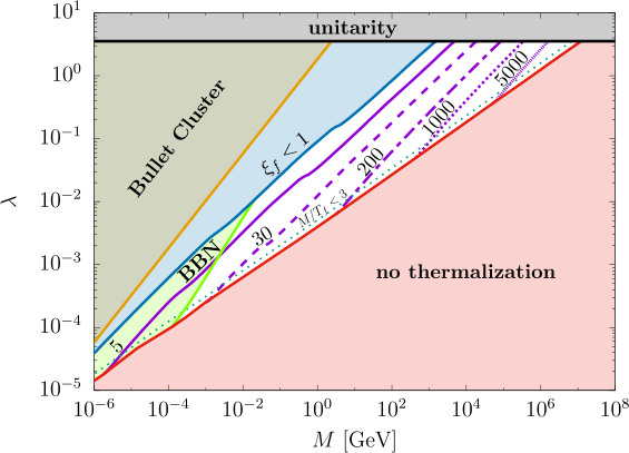
The upper boundary of the relativistic freeze-out region is marked by the green dotted line. In the model at hand, this region is rather small and extends along the border of the ‘‘non-thermalization’’ area. This can be understood qualitatively as follows: smaller couplings lead to earlier freeze-out (since ) and, thus, more significant relativistic effects for a fixed . On the other hand, thermalization is more difficult to achieve at such couplings, so that relativistic freeze-out turns out to be only barely compatible with thermal equilibrium. In contrast, in the scalar dark matter model [19], relativistic freeze-out dominates the allowed parameter space due to a much stronger Bose-Einstein enhancement of the rates.
In the deep non-relativistic regime, the main parameter dependence of the correct relic density curves is captured by
| (27) |
This follows from the freeze-out relation . More precisely, the right hand side of the above equation should be multiplied by , which varies rather slowly in the non-relativistic regime.55 5 Part of this -dependence comes from the velocity suppression of the neutrino annihilation cross section. For relativistic freeze-out, the relic density lines tend to curve down towards vertical lines since in this case becomes almost independent of .
In the allowed region, dark matter is cold: for very light , keV, the dark sector is significantly cooler than the SM thermal bath, while for heavier DM (above 10 MeV), the dark temperature is comparable to or lower than . Therefore, in either case DM is non-relativistic at the structure formation temperature around 1 keV.
We conclude that viable sterile neutrino masses in our model range from about keV to as much as TeV, without violating perturbativity. This in contrast to the usual WIMP mass upper bound of order 10 TeV imposed by perturbative unitarity. The difference stems from the fact that the dark sector can be much colder than the observable one, which suppresses the necessary (see Eq. 27). This was also observed in [47] in a more general context. In the scalar DM model [19], however, an analogous effect is not as pronounced due to a different dependence and the upper bound on the DM mass is of order 100 TeV.
Finally, let us comment on observational prospects of sterile neutrino DM. Indirect detection is hindered by the velocity suppression of , which reduces the corresponding cross section by 6 orders of magnitude (see, however, [48]) and makes this detection mode unlikely. Direct detection prospects are also dim, although they depend on the -decay mechanism. If does not have any significant coupling to fermions, the direct detection cross section is negligibly small. Otherwise, it is suppressed by at least or , where is the effective theory cut-off and is a possible singlet-Higgs mixing angle. On the other hand, the sterile neutrino decay can produce an observable signal in a wide range of photon frequencies, whose intensity depends on the active-sterile neutrino mixing angle (Fig. 2).
5 Conclusion
We have studied thermal sterile neutrinos as dark matter candidates in a singlet-extended Standard Model. If the dark sector is cooler than the SM thermal bath, the freeze out mechanism can account for the correct DM abundance, be it relativistic or non-relativistic freeze out. In order to study the relativistic regime, we have obtained the reaction rates which include the Fermi-Dirac and Bose-Einstein quantum statistical factors as well as dependence on the effective chemical potential. This allows us to analyze the freeze-out process in detail as well as obtain the necessary thermalization condition. Our main results are presented in Fig. 6. We conclude that the relativistic freeze-out regime is limited to a narrow band close to the thermalization bound. Quantum statistics effects are important for deriving the latter. Dark matter is cold and the allowed sterile neutrino masses range from MeV to TeV. Such heavy neutrinos are not in conflict with perturbativity as long as the dark sector is much colder than the observable one.
While prospects of direct detection of neutrino DM are rather dim, its decay can potentially be observed for a range of tiny active-sterile mixing angles (Fig. 2).
Acknowledgements. We are grateful to Valentina De Romeri for collaborating at the early stages of the project and providing us with Fig. 2.
This work was supported by the JSPS Grant-in-Aid for Scientific Research
KAKENHI Grant No. JP20K22349 (TT).
References
- [1] P. Minkowski, Phys. Lett. 67B, 421 (1977).
- [2] M. Gell-Mann, P. Ramond and R. Slansky, Conf. Proc. C 790927, 315 (1979).
- [3] T. Yanagida, Conf. Proc. C 7902131, 95 (1979).
- [4] R. N. Mohapatra and G. Senjanovic, Phys. Rev. Lett. 44, 912 (1980).
- [5] J. Schechter and J. W. F. Valle, Phys. Rev. D 22, 2227 (1980).
- [6] G. Lazarides, Q. Shafi and C. Wetterich, Nucl. Phys. B 181, 287 (1981).
- [7] S. Dodelson and L. M. Widrow, Phys. Rev. Lett. 72, 17 (1994).
- [8] X. D. Shi and G. M. Fuller, Phys. Rev. Lett. 82, 2832 (1999).
- [9] K. Abazajian, G. M. Fuller and M. Patel, Phys. Rev. D 64, 023501 (2001).
- [10] T. Asaka, S. Blanchet and M. Shaposhnikov, Phys. Lett. B 631, 151 (2005).
- [11] T. Asaka, M. Laine and M. Shaposhnikov, JHEP 0701, 091 (2007); Erratum: [JHEP 1502, 028 (2015)].
- [12] A. Kusenko, Phys. Rev. Lett. 97, 241301 (2006).
- [13] K. Petraki and A. Kusenko, Phys. Rev. D 77, 065014 (2008).
- [14] R. S. L. Hansen and S. Vogl, Phys. Rev. Lett. 119, no.25, 251305 (2017).
- [15] J. Herms, A. Ibarra and T. Toma, JCAP 06, 036 (2018).
- [16] C. Jaramillo, M. Lindner and W. Rodejohann, JCAP 04, 023 (2021).
- [17] G. Arcadi, J. P. Neto, F. S. Queiroz and C. Siqueira, Phys. Rev. D 105, no.3, 035016 (2022).
- [18] R. Coy and M. A. Schmidt, JCAP 08, 070 (2022).
- [19] G. Arcadi, O. Lebedev, S. Pokorski and T. Toma, JHEP 08, 050 (2019).
- [20] O. Lebedev, Prog. Part. Nucl. Phys. 120, 103881 (2021).
- [21] V. De Romeri, D. Karamitros, O. Lebedev and T. Toma, JHEP 10, 137 (2020).
- [22] P. Bandyopadhyay, M. Mitra and A. Roy, JHEP 05, 150 (2021).
- [23] T. Bringmann, S. Heeba, F. Kahlhoefer and K. Vangsnes, JHEP 02, 110 (2022).
- [24] M. Drewes and J. U. Kang, JHEP 05, 051 (2016).
- [25] I. Flood, R. Porto, J. Schlesinger, B. Shuve and M. Thum, Phys. Rev. D 105, no.9, 095025 (2022).
- [26] E. Fernandez-Martinez, M. Pierre, E. Pinsard and S. Rosauro-Alcaraz, Eur. Phys. J. C 81, no.10, 954 (2021).
- [27] G. Bélanger, S. Khan, R. Padhan, M. Mitra and S. Shil, Phys. Rev. D 104, no.5, 055047 (2021).
- [28] O. Seto and T. Shimomura, Phys. Lett. B 811, 135880 (2020).
- [29] S. Eijima, O. Seto and T. Shimomura, Phys. Rev. D 106, no.10, 103513 (2022).
- [30] M. Pospelov, A. Ritz and M. B. Voloshin, Phys. Lett. B 662, 53-61 (2008).
- [31] A. Boyarsky, O. Ruchayskiy and M. Shaposhnikov, Ann. Rev. Nucl. Part. Sci. 59, 191 (2009).
- [32] A. Boyarsky, M. Drewes, T. Lasserre, S. Mertens and O. Ruchayskiy, Prog. Part. Nucl. Phys. 104, 1-45 (2019).
- [33] O. Lebedev, JCAP 02, 032 (2023).
- [34] J. R. Ellis and O. Lebedev, Phys. Lett. B 653, 411-418 (2007).
- [35] E. W. Kolb and M. S. Turner, Front. Phys. 69, 1-547 (1990).
- [36] J. Bernstein, ‘‘Kinetic theory in the expanding Universe,’’ Cambridge University Press, Cambridge, 1988.
- [37] J. Bernstein, L. S. Brown and G. Feinberg, Phys. Rev. D 32, 3261 (1985).
- [38] P. Gondolo and G. Gelmini, Nucl. Phys. B 360, 145-179 (1991).
- [39] O. Lebedev and T. Toma, Phys. Lett. B 798, 134961 (2019).
- [40] A. Belyaev, N. D. Christensen and A. Pukhov, Comput. Phys. Commun. 184, 1729-1769 (2013).
- [41] J. König, A. Merle and M. Totzauer, JCAP 11, 038 (2016).
- [42] P. A. R. Ade et al. [Planck], Astron. Astrophys. 594, A13 (2016).
- [43] E. D. Carlson, M. E. Machacek and L. J. Hall, Astrophys. J. 398, 43-52 (1992).
- [44] S. Andreas, O. Lebedev, S. Ramos-Sanchez and A. Ringwald, JHEP 08, 003 (2010).
- [45] A. Fradette, M. Pospelov, J. Pradler and A. Ritz, Phys. Rev. D 99, no.7, 075004 (2019).
- [46] A. Robertson, R. Massey and V. Eke, Mon. Not. Roy. Astron. Soc. 465, no.1, 569-587 (2017).
- [47] R. Coy, T. Hambye, M. H. G. Tytgat and L. Vanderheyden, Phys. Rev. D 104, no.5, 055021 (2021).
- [48] C. Johnson, R. Caputo, C. Karwin, S. Murgia, S. Ritz and J. Shelton, Phys. Rev. D 99, no.10, 103007 (2019).