Optimization of Cartesian Tasks with Configuration Selection
Abstract
A basic task in the design of an industrial robot application is the relative placement of robot and workpiece. Process points are defined in Cartesian coordinates relative to the workpiece coordinate system, and the workpiece has to be located such that the robot can reach all points. Finding such a location is still an iterative procedure based on the developers’ intuition. One difficulty is the choice of one of the several solutions of the backward transform of a typical 6R robot. We present a novel algorithm that simultaneously optimizes the workpiece location and the robot configuration at all process points using higher order optimization algorithms. A key ingredient is the extension of the robot with a virtual prismatic axis. The practical feasibility of the approach is shown with an example using a commercial industrial robot.
Keywords:
configuration, virtual axis, differentiable optimization1 Problem Statement
When programming an industrial robot application the typical workflow starts with the workpiece that has to be processed. The process points like welding points, drilling holes, points describing a glueing or laser contour are defined. For handling applications also points are defined, not relative to the transported workpiece, but to devices holding and transporting the items. The points are actually frames in relative to the workpiece frame . Then the application developer chooses a robot, and the workpiece location relative to the robot.
The difficulty is as follows: A typical industrial robot with up to 8 discrete solutions, one has to be chosen individually for each process point according to some criterion, solvability being the first. We call these solutions in axis space configurations , with a finite set coding the possible configurations like . In industrial robot programming languages frame data are extended by a code for the configuration selection. E.g. the KRL language KSS83SI uses an integer named status, abbreviated S, whose bits 0,1 and 2 code sign choices in the backward transform. A point-to-point command then looks like
PTP {X 100, Y 200, Z 300, A 40, B 50, C 60, S ’B101’}
with components A, B, C as Euler-like angles . Other robot languages use different terms and syntax but the underlying mathematics is the same.
The configuration information is not a part of the Cartesian data so actually an additional degree of freedom comes from the backward transform. But it is not intuitive for humans which solution falls into axis limits due to mechanical design, which may have to be restricted further according to the cell setup or cabling of the robot. So not all of the 8 solutions may reachable, even in an asymmetric way as axis ranges are not symmetric around . So making all points reachable for the robot is still based on human intuition and trial-and-error. It would be desirable to have an algorithm which, given process frames
expressed in a frame , and a robot description, determines a reachable workpiece position in world and suitable configurations for all .
In Wei.2019 we have presented an algorithm which solves the task described so far with an extension of the 6R robot to a RRRPRRR robot with a virtual prismatic axis that makes all of reachable, if we drop axis restrictions in addition. The virtual axis measures non-reachability from the original robot perspective. If a location is found with the virtual axis set to 0 for all positions, and all axes are inside their ranges, then the problem is also solved for original robot. However this algorithm only works with the restrictive assumption that all are approached with the same configuration . In this paper we extend the approach to different configurations for each , still determined by efficient algorithms from differentiable optimization. Approaches with virtual axes are also used e.g. in GeuFlores.2019; Leger.2016; Pellegrino.2020 but the configuration is explicitly held fixed in these papers. Automatic selection of the robot configuration is new to the best of the author’s knowledge.
The paper is organized as follows: In Section 2 we introduce notation and briefly present the virtual axis approach. Section 3 explains the formulation of the optimization problem with the discrete configuration set suitable for solvers using derivatives. Numerical results with data from a industrial robot are shown in Section 4 before we summarize and conclude with directions for further research.
2 Virtual Axis Approach


We consider a 6R robot with spherical wrist and kinematic structure typical of many industrial robots. The robot is modelled in the Denavit-Hartenberg convention of the Robotics Toolbox described in Corke.2011: The frame relating the coordinate systems of axes and is
with the usual abbreviations for translations and rotations. In addition to the familiar , , , the offset gives an additional degree of freedom to assign the axis zero positions as the mechanical engineers prefer.
We use a KUKA KR6R900 robot KSS83SI industrial robot with 6 kg payload and 900 mm reach. A construction drawing with the robot in its home position as well as the axis sense of rotation are shown in Figure 1, parameters and axis limits in Table 1 derived from AgilusSpecification.2013. Note that axis 1 is pointing downward in the manufacturers definition, so the kinematic chain starts with an additional .
This robot is mapped to a virtual robot with an additional prismatic joint with variable between the original axes 3 and 4, shown in the same Table 1 with tildes over the variables. We distinguish between the variables of the two robots with indices and , and respectively. Ignoring axis limits and singularites, the backward transform gives up to 8 discrete solutions indexed by . The virtual robot axis ranges are for all rotational axes, and for the virtual axis.
| type | ||||||||||
|---|---|---|---|---|---|---|---|---|---|---|
| 1 | 1 | -400 | 25 | 0 | R | |||||
| 2 | 2 | 0 | 455 | 0 | 0 | R | ||||
| 3 | 3 | 0 | 35 | R | ||||||
| 4 | 0 | 0 | 0 | 0 | 0 | P | ||||
| 4 | 5 | -420 | 0 | 0 | R | |||||
| 5 | 6 | 0 | 0 | 0 | R | |||||
| 6 | 7 | -80 | 0 | 0 | R |
We denote by , the forward transform of the original robot, denoting the set of frames, i. e. in matrix representation. forward returns the tool frame in world coordinates and also the configuration, hereby making forward injective with an inverse backward on the set of nonsingular axis positions. The configuration is a function ; the formulas are not explicitly presented here: Bit 0 of is set if the wrist centre point is behind axis 1. Bit 1 is set if the wrist centre point is below the line connecting axes 2 and 3. Bit 2 is set if axis 5 is directed upward. These bits are not simply signs of axis angles because there are offsets between axis 1 and 2 as well as between axis 3 and 4, so the wrist centre point is not above axis 1 or on the line from axis 2 to 3 if the robot is in an upright position. We overload the meaning of forward and also write for the 7 axis virtual robot. Analogously, backward denotes the backward transform in world coordinates
The special value in the range is used to signal unreachable points when the wrist centre point is outside the working space, or a solution with the given configuration exists, but outside the axis range.
The backward transform of the virtual robot is identical to the standard 6R backward transform, if the TCP frame is reachable for the 6R robot. If not, the virtual axis is elongated to the minimum length (in absolute value) necesssary for the wrist centre point to make the target point reachable; such a solution always exists for our robot class. This gives a well-defined function (for details see Wei.2019, including a smoothing operation at the workspace boundary). The key idea to replace the error signal in the non-solvable case by the quantity of the virtual robot to measure non-solvability of the original backward transform.
Our implementation can handle the class of 6R robots with the values exactly as given in Table 1, and all the , possibly non-zero as in Table 1. The virtual axis could also be inserted between axes 2 and 3 with no effect on the rest of the analysis. Other locations would not work – e. g. before axis 1 or after axis 6 – or change the kinematic structure, e. g. between axes of the central wrist. The approach carries over to any robot class with analytic solution and a similar virtual axis extension.
3 Optimization with Configuration Selection
Given a workpiece frame it is easy to check whether all process frames are reachable: Evaluate the backward transform for each with all possible configurations , , where denotes the change of coordinates from to . If at least one solution exists for all , choose any of these solutions. If however at least one exists such that signals an unreachable frame for all configurations , we have no mathematical clue how to change . This clue now comes from the virtual axis value .
We explain the algorithm in three steps: First we reformulate the reachability check for a single as a minimization problem, without axis restrictions. Then axis ranges are included. Finally we consider several and variations.
minimin problem
Given a single TCP frame , reachability for workpiece location can be expressed for the original robot as follows: There exists such that . For the virtual robot this is equivalent to: There exists such that where , and is the projection onto the -component. Abbreviating , this can be rephrased as as a minimization problem as in Wei.2019: If has minimum value 0, we have found a reachable solution. The square gives differentiability but can be replaced by the absolute value or any other distance function. The nondifferentiability of the absolute value can also be handled in the optimization problem, see Section 4.
However, we have to optimize over giving (Note that is not the problem we are interested in: this means different positions for each configuration). This is a minimin-optimization problem considered difficult in literature, because the minimum over a finite number of differentiable functions is not differentiable but only continuous. This seems to exclude optimizers using derivatives that wen want to employ for efficiency.
So we have to reformulate the problem. For unconstrained minimax problems like the minimization of the -norm there exist standard transformations to smooth, even linear, but constrained formulations, see textbooks like Luenberger.2016. For minimin, (Nocedal.2006, Exercise 12.6) leaves the problem unanswered, hinting that no differentiable formulation exists. (Eiselt.2007, Chapter 8) suggests a sequence of linear problems, one for each , but only for a linear original problem. A key developer of the Gurobi optimization package suggests mixed nonlinear-integer programming GregGlockner.2016, with a bit for each encoding with whether attains the minimum, and an additional constraint enforcing exactly one minimizing function. This excludes a variable number of functions reaching the minimum simultaneaously, and requires specialized software.
We propose a different transformation to a smooth constrained problem – as smooth as the – with a convex combination which seems to be new. We state the lemma with as the standard optimization variable, in our application any parametrization of the workpiece frame with .
Lemma 1
Consider for , a finite set. Consider the unconstrained minimization problem
| (1) |
and the constrained problem
| (2) | ||||
| subject to |
Then the problems are equivalent: (1) is unbounded iff (2) is. If the problems are bounded, then the minimum and infimum values are the same, for some if the minimum is attained.
Proof
The constraint enforces that at least one function attains its minimum, if a minimum exists.
Assume a finite minimum for some for (1). We show that and with and for all is optimal for (2). Clearly are admissible with objective function value . Choose any admissible. The are nonnegative and sum to 1, so we get
Therefore cannot attain a smaller objective value.
In the other direction, assume a finite minimum for (2) at , . If for several , then all corresponding must take the same value - otherwise we could choose the minimum over , increase the corresponding weight , adjust the convex combination and so reduce the objective value. But with identical function values we can move the weights in to a singleton with , otherwise. As before is the minimum point for (1). The arguments for infimum and unboundedness are similar.
Axis range restrictions
Now we can include axis constraints into the smooth reformulation of the minimin problem. We sill consider a single process frame . We identify where is the virtual axis value from , assuming no constraints on the axes, and now with depending on . If , then is reachable for at least one configuration.
However the axis constraints are special: We need only for those configurations with : If needs an elongated virtual axis, then is unreachable anyway for the original robot anyway, no matter whether the original axes restrictions are fulfilled. We model this with a slack variable for the violation of the axis restrictions for configuration , which is also included in the objective function (we suppress the dependence of on ):
| subject to | ||||||
| (3) | ||||||
If all axis restrictions can be met with we have found a solution for the original robot. With the same argument as in the minimin lemma an objective value 0 signals reachability for at with at least one configurations. The measures for violation of workspace and for violation of axis range are nonnegative, yielding 0 for a reachable pose for the original robot. Summing this up, we have replaced the test whether is reachable by a optimization problem to find and respectively. Individual slack variables and for all axis constraints would also do but increase the number of variables.
If several reach the same minimum value, then the proof of the Lemma shows that any configuration with can be chosen in the application, this is still a degree of freedom.
Formulation with frame list and variations
For the original problem with several frames we simply add indices to the variables , , , of (3) (but not , which describes the single workpiece) and sum over all frames in the objective function .
Note that then we still only have one slack variable for each configuration at each , measuring axis range violations. This is the correct formulation for path point-to-point processes like handling. For path processes with blending contours a change of configuration must not occur on a path enclosed by two stop points because this would mean that a singularity is crossed. However this requirement can be modelled easily: We use one common slack variable for all on the same path segment, but different variables for different segments.
User constraints on , like a rectancle of possible positions on a table, can be expressed in with easily.
4 Numerical Results
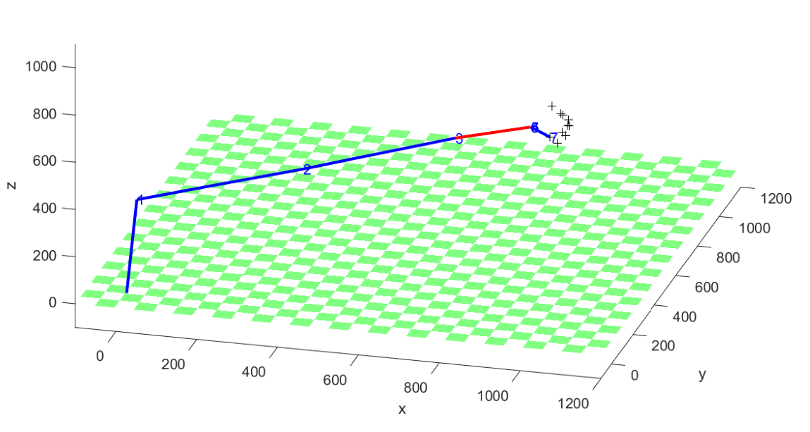
We have implemented the optimization problem in MATLAB with the SQP solver of the Optimization Toolbox. For problems around a solution is found in typically less than 5 minutes on a standard laptop with i7 processor, with parallel evaluation of the computations for the . Figure 2 shows a typical initial and optimized positions. The virtual axis is plotted in red, so the robot is reaching to an unreachable point in the initial setup. In the optimized solution, makes the virtual axis invisible.
We have also compared minimizing the absolute value instead of using the standard transformation , with from linear programming, giving . Numerical experiments showed better overall performance because has small derivatives near the optimium, slowing down progress. The additional variables , for all and increase computation time for derivatives but reduced the number of iterations significantly. Due to the nonlinearity of the problem, the solver sometimes got stuck in an non-reachable workpiece frame.

5 Conclusion and Outlook
We have presented a general purpose algorithms that places a workpiece in the reachable workspace of a 6R industrial robot, capaple of selecting configurations for all process points. A natural next step is a time optimal path through one of the possible configurations of each process point in a travelling salesman approach Laporte.1983. We found no academic software that offers configuration programming at all. In the author’s opinion, this would be a very useful functionality.
References
- (1) Corke, P.: Robotics, Vision and Control: Fundamental Algorithms in MATLAB. Springer (2011)
- (2) Eiselt, H.A., Sandblom, C.L.: Linear Programming and its Applications. Springer-Verlag Berlin Heidelberg, Berlin, Heidelberg (2007). DOI 10.1007/978-3-540-73671-4. URL http://site.ebrary.com/lib/alltitles/docDetail.action?docID=10189321
- (3) Geu Flores, F., Röttgermann, S., Weber, B., Kecskeméthy, A.: Generalization of the virtual redundant axis method to multiple serial-robot singularities. In: V. Arakelian, P. Wenger (eds.) ROMANSY 22 - Robot design, dynamics and control, CISM International Centre for Mechanical Sciences, Courses and Lectures Courses and lectures, vol. 584, pp. 499–506. Springer, Cham (2019)
- (4) Greg Glockner: How to covert min min problem to linear programming problem? (2016). URL https://math.stackexchange.com/questions/1858740/how-to-covert-min-min-problem-to-linear-programming-problem
- (5) KUKA Roboter GmbH: KR AGILUS sixx specification (2013)
- (6) KUKA Roboter GmbH: KUKA system software 8.3: Operating and programming instructions for system integrators (2015)
- (7) Laporte, G., Nobert, Y.: Generalized travelling salesman problem through n sets of nodes: An integer programming approach. INFOR: Information Systems and Operational Research 21(1), 61–75 (1983). DOI 10.1080/03155986.1983.11731885
- (8) Léger, J., Angeles, J.: Off-line programming of six-axis robots for optimum five-dimensional tasks. Mechanism and Machine Theory 100, 155–169 (2016)
- (9) Luenberger, D.G., Ye, Y.: Linear and Nonlinear Programming, International Series in Operations Research & Management Science, vol. 228, 4th ed. 2016 edn. Springer International Publishing and Imprint: Springer, Cham (2016)
- (10) Nocedal, J., Wright, S.J.: Numerical Optimization, 2 edn. Springer, New York (2006)
- (11) Pellegrino, F.A., Vanzella, W.: Virtual redundancy and barrier functions for collision avoidance in robotic manufacturing. In: 2020 7th International Conference on Control, Decision and Information Technologies (CoDIT), vol. 1, pp. 957–962 (2020). DOI 10.1109/CoDIT49905.2020.9263936
- (12) Weiß, M.: Optimal object placement using a virtual axis. In: J. Lenarcic, V. Parenti-Castelli (eds.) Advances in Robot Kinematics 2018, Springer Proceedings in Advanced Robotics, vol. 8, pp. 116–123. Springer International Publishing, Cham (2019)