跳到论文正文
W Papers独立论文阅读器 arXiv:2302.09265 论文正文 计算阅读时间 · 0%
引用这篇论文根据当前论文元数据生成,正式投稿前建议核对。


License: arXiv.org perpetual non-exclusive license
arXiv:2302.09265v1 [cs.ET] 18 Feb 2023

Diffusive Molecular Communication with a Spheroidal Receiver for Organ-on-Chip Systems
Thanks: ©2023 IEEE. Personal use of this material is permitted. Permission from IEEE must be obtained for all other uses, in any current or future media, including reprinting/republishing this material for advertising or promotional purposes, creating new collective works, for resale or redistribution to servers or lists, or reuse of any copyrighted component of this work in other works.

Hamidreza Arjmandi1, Mohamad Zoofaghari2, Mitra Rezaei1,
Kajsa Kanebratt3, Liisa Vilen3, David Janzen4, Peter Gennemark3,5, and Adam Noel1
Affiliation: 1School of Engineering, University of Warwick, Coventry, UK.
2Electrical Engineering Department, Yazd University, Yazd, Iran.
3Drug Metabolism and Pharmacokinetics, Research and Early Development, Cardiovascular, Renal and Metabolism (CVRM),
Bio-Pharmaceuticals, R&D, AstraZeneca, Gothenburg, Sweden.
4Clinical Pharmacology and Quantitative Pharmacology, Clinical Pharmacology and Safety Sciences,
AstraZeneca AB R&D Gothenburg, Gothenburg, Sweden.
5Department of Biomedical Engineering, Linköping University, Sweden.
Abstract

Realistic models of the components and processes are required for molecular communication (MC) systems. In this paper, a spheroidal receiver structure is proposed for MC that is inspired by the 3D cell cultures known as spheroids being widely used in organ-on-chip systems. A simple diffusive MC system is considered where the spheroidal receiver and a point source transmitter are in an unbounded fluid environment. The spheroidal receiver is modeled as a porous medium for diffusive signaling molecules, then its boundary conditions and effective diffusion coefficient are characterized. It is revealed that the spheroid amplifies the diffusion signal, but also disperses the signal which reduces the information communication rate. Furthermore, we analytically formulate and derive the concentration Green’s function inside and outside the spheroid in terms of infinite series-forms that are confirmed by a particle-based simulator (PBS).

Index Terms: 
Molecular communication, Spheroid, Organ-on-chip, Diffusion.

I Introduction

Molecular communication (MC) is a bio-inspired mechanism that is envisioned to realize micro- and nano-scale communication systems using molecules as information carriers [1]. Despite many efforts by the MC community to model the components of MC systems, more realistic models are required. Elements and structures of in vitro environments such as organs-on-chip could be used to improve model realism, potentially contribute to MC research and development, and to provide mechanistic insight into the biology of the organs (on the chip).

Existing literature over-simplifies the MC receiver in a biological environment and does not sufficiently account for the interactions of signaling molecules with the environment and the biological or biosynthetic receivers and transmitters (i.e., cells). The passive receiver, in which information molecules freely diffuse in the receiver’s space and the movement of molecules is not affected, is the most common model used in previous works [2]. Such a simple model is often used to facilitate analysis of other aspects of a MC system, e.g., the environment boundary [3]. The passive model may be relevant for small and hydrophobic molecules (which are repelled from water molecules) that easily pass through a cell membrane. However, most extracellular molecules are too large or too hydrophilic to traverse the cell membrane [4] and also cells usually react with signaling molecules (either directly on the surface or in the intracellular environment).

To address the limitations of the passive receiver model, some works have considered a reception mechanism across the receiver (cell) membrane activating a signaling pathway (i.e., a series of chemical reactions controlling a cell function). These works have studied the effects of various types of reactions across the membrane, as well as the size, number, spatial distribution, and/or saturation of the receptors on the cell membrane [5, 6, 7, 8, 9, 10, 11].

Previous works have considered the receiver as a single cell (or machine) whose surface is reacting with molecules. However, cells do not normally live in isolation but in populations with other cells of the same or of different types. This is true in vivo but also in many in vitro systems. In particular, tissues and tumors in multi-cellular organisms and biofilms of microorganisms are common natural instances whereas spheroids, organoids, tumoroids, and cell islets are well-known instances in biological experimental setups. This inspires the design of MC transceivers based on a population of (biological or biosynthetic) cells. In [12], the authors consider an implantable drug delivery system inside a spherical tumor microenvironment releasing drug molecules and obtain the spatiotemporal drug concentration profile in the surrounding tissue.

One realistic receiver for MC is a spheroid structure, which is a 3D cell aggregation in a spherical shape that is widely used in organ-on-chip systems. Spheroids are constructed by various methods aiming to emulate the internal physiological activities of an organ [13]. In this paper, we consider a diffusive MC system with a spheroidal receiver and a point source transmitter. We model the spheroidal receiver as a porous medium for the diffusion signal and characterize its effective diffusion coefficient and implied boundary condition. We introduce and characterize two important processing features of the spheroid: amplification and dispersion of the diffusion signal. Furthermore, we obtain the concentration Green’s function in an unbounded environment in the presence of the spheroidal receiver. Our results are confirmed by a particle based simulator (PBS).

The rest of the paper is organized as follows. Section II describes the spheroid structure and diffusive MC system. In Section III, the spheroid Green’s function is provided. Results and discussions are presented in Section IV. Finally, Section V concludes the paper.

II System Model

II-A Spheroid model

A spheroid with radius RsR_{s} formed by NcN_{c} cells is considered. The spheroid interior space is comprised of the cells and the void space between the cells (i.e., extracellular environment). Given that the volume of a cell within the spheroid is VcV_{c}, the volumes of the cell matrix and the void space inside the spheroid are given by Vc​NcV_{c}N_{c} and Vs−Vc​NcV_{s}-V_{c}N_{c}, respectively, where Vs=43​π​Rs3V_{s}=\frac{4}{3}\pi R_{s}^{3} is the spheroid volume.

We model the spheroid structure as a porous medium with volume VsV_{s} whose porosity, ϵ\epsilon, is defined as the ratio of the void space to the whole spheroid volume, i.e.,

ϵ=1−Nc​VcVs.\displaystyle\epsilon=1-\frac{N_{c}V_{c}}{V_{s}}. (1)

We assume that the spheroid is in a fluid medium that surrounds it and fills its void space. The diffusive signaling molecules of type AA in the medium can diffuse into the void space of the spheroid and stimulate the spheroid’s cells through a transmembrane mechanism, e.g., by binding to receptors.

Inside the spheroid, the molecules diffuse via the curved paths of the void space among the cells, which leads to a shorter net displacement of the molecules in a given time interval. Thus, macroscopic diffusion within the spheroid effectively differs from the diffusion within the free fluid outside the spheroid. Since the molecules traverse a shorter net path within the spheroid, the effective diffusion coefficient is smaller than the diffusion coefficient in the free fluid medium and molecules are more likely to be observed and sensed by the spheroid’s cells. Given the diffusion coefficient DD for molecules AA in the free fluid, the effective diffusion coefficient within the spheroid is given by

Deff=ϵτ​D,\displaystyle D_{\rm eff}=\frac{\epsilon}{\tau}D, (2)

where τ\tau is the tortuosity, a measure of the transport properties of the porous medium, and is modeled as a function of spheroid porosity as τ=1ϵ0.5\tau=\frac{1}{\epsilon^{0.5}} [14].

To describe the environment geometry, we use the spherical coordinate system where (r,θ,φ)(r,\theta,\varphi) denote radial, elevation, and azimuth coordinates, respectively. At the border of the two diffusive environments with different diffusion coefficients, we have a flow continuity condition as

Deff​∂cs​(r¯,t)∂r=D​∂co​(r¯,t)∂r,\displaystyle D_{\rm eff}\frac{\partial c_{s}(\bar{r},t)}{\partial r}=D\frac{\partial c_{o}(\bar{r},t)}{\partial r}, (3)

and another boundary condition that is generally modeled as [15, Ch. 3]

cs​(r¯,t)=k​co​(r¯,t),\displaystyle c_{s}(\bar{r},t)=kc_{o}(\bar{r},t), (4)

where r¯∈∂Ω\bar{r}\in\partial\Omega, ∂Ω\partial\Omega denotes the boundary region of the spheroid, and csc_{s} and coc_{o} denote the concentration function inside and outside the spheroid, respectively. The constant kk is a function of porosity of the medium and should be determined experimentally. But, the literature on mathematical analysis of tumor spheroids simply assumes continuity of concentration, i.e., k=1k=1, by neglecting the porosity of the medium [16, 17]. However, in the results section, we show using a PBS that for two ideal diffusion environments with diffusion coefficients DD and DeffD_{\rm eff}, we have k=DDeffk=\sqrt{\frac{D}{D_{\rm eff}}}. Thus, for k≠1k\neq 1, a concentration discontinuity (i.e., jump) occurs at the boundary.

Refer to caption
Fig. 1: Porosity (ϵ\epsilon) and concentration ratio at the boundary (kk) versus the number of cells inside the spheroid (NcN_{c}).

Fig. 1 demonstrates the porosity (ϵ\epsilon) and boundary concentration ratio (kk) as a function of the number of the cells, 15000<Nc<2500015000<N_{c}<25000 in the spheroid when the spheroid radius and cell volume are assumed to be Rs=275R_{s}=275 μ​m\mu\mathrm{m} and Vc=3.14×10⁻¹⁵V_{c}=3.14\times 10^{-15} m3\mathrm{m}^{3}, respectively [18]. As observed in Fig. 1, the boundary concentration ratio increases exponentially with an increase in NcN_{c}. For Nc=24000N_{c}=24000, which is the approximate number of cells in HepaRG spheroids reported in [18], we have ϵ=0.13\epsilon=0.13 and correspondingly k=4.49k=4.49. This value of k suggests a large concentration discontinuity at the spheroid boundary.

We assume that the molecules may bind to cell receptors through a chain of reactions leading to product molecules EE that are counted by cells, i.e.,

whereBa​n​dandEm​a​y​r​e​p​r​e​s​e​n​t​t​h​e​r​e​c​e​p​t​o​r​m​o​l​e​c​u​l​e​s​a​n​d​t​h​e​f​i​n​a​l​p​r​o​d​u​c​t​s​i​n​t​h​e​c​e​l​l​s,r​e​s​p​e​c​t​i​v​e​l​y.A​r​e​a​l​m​a​t​u​r​e​s​p​h​e​r​o​i​d​i​s​t​i​g​h​t​l​y​f​o​r​m​e​d​b​y​a​l​a​r​g​e​n​u​m​b​e​r​o​f​c​e​l​l​s,r​e​s​u​l​t​i​n​g​i​n​a​s​m​a​l​l​p​o​r​o​s​i​t​y.T​h​e​n,a​s​i​g​n​a​l​i​n​g​m​o​l​e​c​u​l​e​m​o​v​i​n​g​w​i​t​h​i​n​t​h​e​v​o​i​d​s​p​a​c​e​w​o​u​l​d​b​e​v​e​r​y​c​l​o​s​e​t​o​t​h​e​c​e​l​l​s′​b​o​u​n​d​a​r​i​e​s​a​n​d​f​r​e​q​u​e​n​t​l​y​e​x​p​o​s​e​d​t​o​b​i​n​d​t​o​r​e​c​e​p​t​o​r​s.T​h​u​s,w​e​a​s​s​u​m​e​t​h​a​t​m​o​l​e​c​u​l​e​s​w​i​t​h​i​n​t​h​e​v​o​i​d​s​p​a​c​e​o​f​t​h​e​s​p​h​e​r​o​i​d​a​r​e​h​o​m​o​g​e​n​e​o​u​s​l​y​a​v​a​i​l​a​b​l​e​f​o​r​t​r​a​n​s​m​e​m​b​r​a​n​e​r​e​a​c​t​i​o​n​s.mayrepresentthereceptormoleculesandthefinalproductsinthecells,respectively.\par Arealmaturespheroidistightlyformedbyalargenumberofcells,resultinginasmallporosity.Then,asignalingmoleculemovingwithinthevoidspacewouldbeveryclosetothecells^{\prime}boundariesandfrequentlyexposedtobindtoreceptors.Thus,weassumethatmoleculeswithinthevoidspaceofthespheroidarehomogeneouslyavailablefortransmembranereactions.\par\par\par

II-B Diffusive MC system with spheroidal receiver

A point-to-point diffusive MC system is considered in which the spheroid is assumed to be the receiver. The spheroid might model a cancer tumor site that should receive drug molecules; it might model the spheroids in a organ-on-chip system that receive nutrient molecules to survive; alternatively, it could be a transceiver nanomachine for information exchange in a MC system.

The spheroid is considered in an unbounded fluid medium and the center of the spheroid is chosen as the origin of the spherical coordinate system. A point source transmitter is located at an arbitrary point r¯tx=(rtx,θtx,φtx)\bar{r}_{\rm tx}=(r_{\rm tx},\theta_{\rm tx},\varphi_{\rm tx}) outside the spheroid. The transmitter uses signaling molecules of type A. A schematic illustration of the system model is represented in Fig. 2.
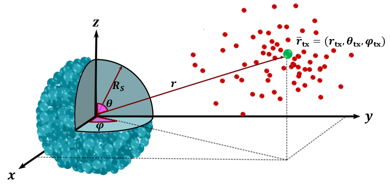
Refer to caption
Fig. 2: System model schematic where the red, greenish-blue, and green spheres represent the signaling molecule, cell, and point source transmitter, respectively.

The released molecules move randomly in the environment following Brownian motion. Their movements are assumed to be independent of each other. The diffusing molecules, which are exposed to the receptors in the spheroid, may bind and generate molecules EE that are counted within the cells in the spheroidal receiver.

The received signal can be defined according to the application. Generally, the cells might respond differently and react to the generated EE molecules. A cell’s response might be a continuous function of product molecule concentration. Then, the received signal in the spheroid may be defined as the aggregate number of generated EE molecules inside the cell. In this case, the concentration profile of EE molecules is obtained as a function of signaling AA molecules based on (II-A). Then, given the uniform density of cells within the spheroid, the received signal is given by

∫0Rs4​π​cE​(r¯,t)​Vc​NcVs​r2​d​r,\displaystyle\int_{0}^{R_{s}}4\pi c_{E}(\bar{r},t)V_{c}\frac{N_{c}}{V_{s}}r^{2}\text{d}r, (5)

where cEc_{E} represents the product molecule concentration. Correspondingly, the received signal can be defined as the total generation rate of the product EE molecules inside the spheroid, i.e., the time derivative of (5). Alternatively, an individual cell might be activated and respond according to a stimulus threshold. For example, if the spheroid is a tumor receiving drug molecules, then each cell might die by receiving a concentration of the drug higher than a threshold. Then, the received signal may be defined as the ratio of killed cells receiving the drug molecules, i.e.,

∫0Rs4​π​IcE​(r¯,t)>𝒯​Vc​NcVs​r2​d​r,\displaystyle\int_{0}^{R_{s}}4\pi I_{c_{E}(\bar{r},t)>\mathcal{T}}V_{c}\frac{N_{c}}{V_{s}}r^{2}\text{d}r, (6)

where I(⋅)I_{(\cdot)} is the indicator function and 𝒯\mathcal{T} is the threshold above which an individual cell is activated.

III Green’s Function Boundary Value Problem

To analyze the presented diffusive MC system, we formulate the corresponding Green’s function boundary value problem for diffusion in the environment. We assume that the point source transmitter, located at an arbitrary point r¯tx=(rtx,θtx,φtx)\bar{r}_{\rm tx}=(r_{\rm tx},\theta_{\rm tx},\varphi_{\rm tx}) outside the spheroid, has an instantaneous molecule release rate11 1 Note that the number of molecules does not have a dimension, so we have not represented it in the units. of δ⁡(t−t0)\delta(t-t_{0}) molecule 1/s1/\rm s, where δ⁡(⋅)\delta(\cdot) is the Dirac delta function. This impulsive point source is represented by the function S⁡(r¯,t,r¯tx,t0)=δ⁡(r−rtx)​δ​(θ−θtx)​δ​(φ−φtx)​δ​(t−t0)r2​sin⁡θS(\bar{r},t,{\bar{r}_{\rm tx}},t_{0})=\frac{{\delta(r-{r_{\rm tx}})\delta(\theta-\theta_{\rm tx})\delta(\varphi-\varphi_{\rm tx})\delta(t-t_{0})}}{r^{2}\sin\theta} s−1​m−3\mathrm{s}^{-1}\,\mathrm{m}^{-3}. Given the source S⁡(r¯,t,r¯tx,t0)S(\bar{r},t,{\bar{r}_{\rm tx}},t_{0}), the molecular diffusion out of the spheroid is described by the partial differential equation (PDE) [19]

D∇2co(r¯,t|r¯tx,t0)+S(r¯,t,r¯tx,t0)=∂co(r¯,t|r¯tx,t0)∂t,\displaystyle D{\nabla^{2}}c_{o}(\bar{r},t|{{\bar{r}}_{\rm tx}},{t_{0}})+S(\bar{r},t,{\bar{r}_{\rm tx}},t_{0})=\frac{{\partial c_{o}(\bar{r},t|{{\bar{r}}_{\rm tx}},{t_{0}})}}{{\partial t}}, (7)

where co(r¯,t|r¯tx,t0)c_{o}(\bar{r},t|{{\bar{r}}_{\rm tx}},{t_{0}}) denotes the molecule concentration at point r¯\bar{r} outside spheroid at time tt. In the rest of the paper, we briefly write coc_{o} instead of co(r¯,t|r¯tx,t0)c_{o}(\bar{r},t|{{\bar{r}}_{\rm tx}},{t_{0}}). In the spherical coordinate system and Fourier domain, (7) is re-written as

Dr2​∂∂r​(r2​∂Co∂r)+Dr2​sin⁡θ​∂∂θ​(sin⁡θ​∂Co∂θ)+Dr2​sin2⁡θ​∂2Co∂φ2\displaystyle\frac{D}{{{r^{2}}}}\frac{\partial}{{\partial r}}\left({r^{2}}\frac{{\partial C_{o}}}{{\partial r}}\right)+\frac{D}{{{r^{2}}\sin\theta}}\frac{\partial}{{\partial\theta}}\left(\sin\theta\frac{{\partial C_{o}}}{{\partial\theta}}\right)+\frac{D}{{{r^{2}}{{\sin}^{2}}\theta}}\frac{{{\partial^{2}}C_{o}}}{{\partial{\varphi^{2}}}} (8)
+δ⁡(r−rtx)​δ​(θ−θtx)​δ​(φ−φtx)​δ​(t−t0)r2​sin⁡θ=i​ω​Co,\displaystyle+\frac{{\delta(r-{r_{\rm tx}})\delta(\theta-\theta_{\rm tx})\delta(\varphi-\varphi_{\rm tx})\delta(t-t_{0})}}{r^{2}\sin\theta}=i\omega C_{o},

where CoC_{o} is the Fourier transform of coc_{o}, ii is the imaginary unit, and ω\omega is the angular frequency variable in the Fourier transform22 2 We use the small cc and capital CC to represent the concentration function in the time and Fourier domains, respectively.. With a first order approximation of the spheroid cell receptor reaction chain (5), the effective diffusion inside the spheroid is modeled as

Deff∇2Cs(r¯,ω|r¯tx,t0)−𝒦(ω)C(r¯,ω|r¯tx,t0)\displaystyle D_{\rm eff}{\nabla^{2}}C_{s}(\bar{r},\omega|{{\bar{r}}_{\rm tx}},{t_{0}})-\mathcal{K}(\omega)C(\bar{r},\omega|{{\bar{r}}_{\rm tx}},{t_{0}}) (9)
=iωCs(r¯,ω|r¯tx,t0),\displaystyle=i\omega C_{s}(\bar{r},\omega|{{\bar{r}}_{\rm tx}},{t_{0}}),

where 𝒦⁡(ω)\mathcal{K}(\omega) is the net impact on molecules A due to the binding process characterized by the reaction chain (II-A). As mentioned, the boundary conditions at the border of the spheroid are given by (3) and (4).

The concentration functions cs(r¯,t|r¯tx,t0)c_{s}(\bar{r},t|{{\bar{r}}_{\rm tx}},{t_{0}}) and co(r¯,t|r¯tx,t0)c_{o}(\bar{r},t|{{\bar{r}}_{\rm tx}},{t_{0}}) that satisfy (7) and (9) subject to the boundary conditions (3) and (4) are called the concentration Green’s functions (CGFs) of diffusion inside and outside the spheroid, respectively. We have solved the problem and obtained the series-form expressions (18) in the Appendix.

IV Results

In this section, we first evaluate the boundary concentration ratio, kk, with a particle based simulator (PBS). We verify the proposed analysis of the spheroid Green’s function using this PBS. Furthermore, we compare the received signal at the spheroidal receiver with a transparent receiver to reveal the signal amplification and dispersion within the spheroid.

The geometric parameters considered in this section are based on the real hepatocyte spheroids used in [18] where the spheroid’s radius is 275 μ\mum with Nc≈24000N_{c}\approx 24000 cells. The volume of one hepatocyte cell is estimated as 3.14×10−153.14\times 10^{-15} m3\mathrm{m}^{3}. The reaction (II-A) inside the spheroid is simply assumed to be an irreversible first order reaction

withk_f=0.01o​r​0.1​s−1.T​h​e​r​e​f​o​r​e,t​h​e​g​e​n​e​r​a​t​i​o​n​r​a​t​e​o​f​t​h​eor0.1$\mathrm{s}^{-1}$.Therefore,thegenerationrateoftheEm​o​l​e​c​u​l​e​s​i​n​s​i​d​e​t​h​e​s​p​h​e​r​o​i​d​i​s​o​b​t​a​i​n​e​d​a​smoleculesinsidethespheroidisobtainedas ∂c E ∂t =k_f c_sa​n​d​c​o​r​r​e​s​p​o​n​d​i​n​g​l​y​t​h​e​t​e​r​mandcorrespondinglythetermK(ω)i​n​(9)​i​s​s​i​m​p​l​yin\eqref{fick2}issimply-k_f.ThePBSisimplementedinMATLAB(R2021b;TheMathWorks,Natick,MA)wherethetimeisdividedintotimestepsof.\par ThePBSisimplementedinMATLAB(R2021b;TheMathWorks,Natick,MA)wherethetimeisdividedintotimestepsofΔt=0.05s.T​h​e​m​o​l​e​c​u​l​e​s​r​e​l​e​a​s​e​d​a​t​t​h​e​p​o​i​n​t​s​o​u​r​c​e​t​r​a​n​s​m​i​t​t​e​r​a​ts.Themoleculesreleasedatthepointsourcetransmitterat ¯ r _tx=(500 μ​m\mu\mathrm{m},π/2,0)m​o​v​e​i​n​d​e​p​e​n​d​e​n​t​l​y​i​n​t​h​e​3−d​i​m​e​n​s​i​o​n​a​l​s​p​a​c​e.T​h​e​d​i​s​p​l​a​c​e​m​e​n​t​o​f​a​m​o​l​e​c​u​l​e​i​nmoveindependentlyinthe3-dimensionalspace.ThedisplacementofamoleculeinΔts​i​s​m​o​d​e​l​e​d​a​s​a​G​a​u​s​s​i​a​n​r​a​n​d​o​m​v​a​r​i​a​b​l​e​w​i​t​h​z​e​r​o​m​e​a​n​a​n​d​v​a​r​i​a​n​c​esismodeledasaGaussianrandomvariablewithzeromeanandvariance2DΔti​n​e​a​c​h​d​i​m​e​n​s​i​o​n​o​f​C​a​r​t​e​s​i​a​n​c​o​o​r​d​i​n​a​t​e​s.F​o​r​t​h​e​P​B​S,t​h​e​s​p​h​e​r​o​i​d​i​s​s​i​m​p​l​y​a​d​i​f​f​u​s​i​o​n​e​n​v​i​r​o​n​m​e​n​t​w​i​t​h​e​f​f​e​c​t​i​v​e​c​o​e​f​f​i​c​i​e​n​tineachdimensionofCartesiancoordinates.ForthePBS,thespheroidissimplyadiffusionenvironmentwitheffectivecoefficientD_eff.Ifthecalculateddisplacementvectorofamoleculeinatimeslotpassesthespheroidboundary,thenthelengthoftheportionofthevectorinsidethespheroidisupdatedbasedontheeffectivediffusioncoefficient.Ifthecalculateddisplacementvectorofamoleculeinatimeslotpassesthespheroidboundary,thenthelengthoftheportionofthevectorinsidethespheroidisupdatedbasedontheeffectivediffusioncoefficientD_eff,i.e.,thatpartofthevectorisscaledbythefactor,i.e.,thatpartofthevectorisscaledbythefactor D eff D .Consideringthereaction(IV)insidethespheroid,amoleculemaybeabsorbedfromthevoidspaceofthespheroidbythecellsduringatimestep.Consideringthereaction\eqref{RC2}insidethespheroid,amoleculemaybeabsorbedfromthevoidspaceofthespheroidbythecellsduringatimestepΔts​w​i​t​h​a​p​p​r​o​x​i​m​a​t​e​p​r​o​b​a​b​i​l​i​t​yswithapproximateprobabilityk_fΔt[20].T​o​s​i​m​u​l​a​t​e​t​h​e​i​m​p​u​l​s​i​v​e​s​o​u​r​c​e,\cite[cite]{[\@@bibref{}{Elka}{}{}]}.Tosimulatetheimpulsivesource,10^6m​o​l​e​c​u​l​e​s​a​r​e​r​e​l​e​a​s​e​d​a​t​t​h​e​t​r​a​n​s​m​i​t​t​e​r​l​o​c​a​t​i​o​n.T​o​o​b​t​a​i​n​a​c​o​n​c​e​n​t​r​a​t​i​o​n​a​t​a​g​i​v​e​n​t​i​m​e​a​n​d​l​o​c​a​t​i​o​n,w​e​a​s​s​u​m​e​a​t​r​a​n​s​p​a​r​e​n​t​s​p​h​e​r​e​c​e​n​t​e​r​e​d​a​t​t​h​a​t​l​o​c​a​t​i​o​n​w​i​t​h​a​s​m​a​l​l​r​a​d​i​u​s​o​f​10​μ​m​a​n​d​c​o​u​n​t​t​h​e​n​u​m​b​e​r​o​f​m​o​l​e​c​u​l​e​s​i​n​s​i​d​e​t​h​e​s​p​h​e​r​e​a​t​t​h​a​t​t​i​m​e.T​h​e​c​o​n​c​e​n​t​r​a​t​i​o​n​w​o​u​l​d​t​h​e​n​b​e​t​h​e​c​o​u​n​t​e​d​n​u​m​b​e​r​o​f​m​o​l​e​c​u​l​e​s​d​i​v​i​d​e​d​b​y​t​h​e​v​o​l​u​m​e​o​f​t​h​e​s​p​h​e​r​e.T​h​e​c​o​n​c​e​n​t​r​a​t​i​o​n​v​a​l​u​e​i​s​n​o​r​m​a​l​i​z​e​d,i.e.,i​s​d​i​v​i​d​e​d​b​ymoleculesarereleasedatthetransmitterlocation.Toobtainaconcentrationatagiventimeandlocation,weassumeatransparentspherecenteredatthatlocationwithasmallradiusof10$\mu\mathrm{m}$andcountthenumberofmoleculesinsidethesphereatthattime.Theconcentrationwouldthenbethecountednumberofmoleculesdividedbythevolumeofthesphere.Theconcentrationvalueisnormalized,i.e.,isdividedby10^6,toobtaintheresponsetotheimpulsivesource. Fig. 3 3 Fig. 3 3CGF at the inner and outer boundaries versus time obtained from the PBS for = N c 24000 . Fig. 3CGF at the inner and outer boundaries versus time obtained from the PBS for = N c 24000 . Fig.showstheconcentrationatinnerandouterboundarypoints,toobtaintheresponsetotheimpulsivesource.\begin{figure}\centering\includegraphics[width]{Fig2.eps} \@@toccaption{{\lx@tag[ ]{{3}}{CGF at the inner and outer boundaries versus time obtained from the PBS for $N_{c}=24000$.}}}\@@caption{{\lx@tag[: ]{{Fig. 3}}{CGF at the inner and outer boundaries versus time obtained from the PBS for $N_{c}=24000$.}}} \@add@centering\end{figure}\par Fig.\ref{Figboundary}showstheconcentrationatinnerandouterboundarypointsc_s(275^- μ​m\mu\mathrm{m}, 0, 0)a​n​dandc_o(275^+ μ​m\mu\mathrm{m}, 0, 0)o​f​t​h​e​s​p​h​e​r​o​i​d​g​i​v​e​n​t​h​e​i​m​p​u​l​s​i​v​e​s​o​u​r​c​e​a​t​t​h​e​t​r​a​n​s​m​i​t​t​e​r​o​b​t​a​i​n​e​d​f​r​o​m​t​h​e​P​B​S​w​h​e​nofthespheroidgiventheimpulsivesourceatthetransmitterobtainedfromthePBSwhenN_c=24000.Wehavealsoplottedtheconcentrationattheouterboundaryscaledbythefactor.Wehavealsoplottedtheconcentrationattheouterboundaryscaledbythefactorkt​o​v​e​r​i​f​y​t​h​e​b​o​u​n​d​a​r​y​c​o​n​d​i​t​i​o​n​(4).T​h​e​m​i​n​o​r​m​i​s​m​a​t​c​h​a​t​t​h​e​p​e​a​k​s​i​s​m​a​i​n​l​y​d​u​e​t​o​t​h​e​P​B​S​p​r​o​c​e​d​u​r​e​t​o​a​p​p​r​o​x​i​m​a​t​e​t​h​e​c​o​n​c​e​n​t​r​a​t​i​o​n​a​t​a​p​o​i​n​t.T​o​c​o​m​p​u​t​e​t​h​e​c​o​n​c​e​n​t​r​a​t​i​o​n​a​t​t​h​e​b​o​u​n​d​a​r​y​p​o​i​n​ttoverifytheboundarycondition\eqref{BC1}.TheminormismatchatthepeaksismainlyduetothePBSproceduretoapproximatetheconcentrationatapoint.Tocomputetheconcentrationattheboundarypoint(275 μ​m\mu\mathrm{m}, 0, 0),wehaveassumedatransparentsphereofradius,wehaveassumedatransparentsphereofradius10  μ​m\mu\mathrm{m}c​e​n​t​e​r​e​d​a​t​t​h​e​b​o​u​n​d​a​r​y​p​o​i​n​t​a​n​d​h​a​v​e​c​o​u​n​t​e​d​t​h​e​m​o​l​e​c​u​l​e​s​i​n​t​h​e​l​e​f​t​a​n​d​r​i​g​h​t​h​e​m​i​s​p​h​e​r​e​t​o​a​p​p​r​o​x​i​m​a​t​e​t​h​e​c​o​n​c​e​n​t​r​a​t​i​o​n​o​f​t​h​e​m​o​l​e​c​u​l​e​s​a​t​i​n​n​e​r​a​n​d​o​u​t​e​r​p​o​i​n​t​s.T​h​i​s​l​e​a​d​s​t​o​s​l​i​g​h​t​l​y​h​i​g​h​e​r​a​n​d​l​o​w​e​r​a​p​p​r​o​x​i​m​a​t​i​o​n​s​f​o​r​t​h​e​c​o​n​c​e​n​t​r​a​t​i​o​n​s​a​t​t​h​e​o​u​t​e​r​a​n​d​i​n​n​e​r​b​o​u​n​d​a​r​y,r​e​s​p​e​c​t​i​v​e​l​y.F​i​g.​d​e​p​i​c​t​s​t​h​e​c​o​n​c​e​n​t​r​a​t​i​o​n​a​t​d​i​f​f​e​r​e​n​t​p​o​i​n​t​s​i​n​s​i​d​e​t​h​e​s​p​h​e​r​o​i​d​a​l​r​e​c​e​i​v​e​r​o​b​t​a​i​n​e​d​f​r​o​m​t​h​e​a​n​a​l​y​s​i​s​p​r​o​v​i​d​e​d​i​n​t​h​e​A​p​p​e​n​d​i​x​a​n​d​a​l​s​o​t​h​e​P​B​S​w​h​e​ncenteredattheboundarypointandhavecountedthemoleculesintheleftandrighthemispheretoapproximatetheconcentrationofthemoleculesatinnerandouterpoints.Thisleadstoslightlyhigherandlowerapproximationsfortheconcentrationsattheouterandinnerboundary,respectively.\par\par\par Fig.\ref{FigCGF}depictstheconcentrationatdifferentpointsinsidethespheroidalreceiverobtainedfromtheanalysisprovidedintheAppendixandalsothePBSwhenN_c=24000.Asobserved,thePBSfullyconfirmstheanalyticalresults.Thefigurealsoindicatesthattheconcentrationsignalweakenssignificantlyatthepointsclosertothespheroidcenterandfartherfromthepointsource.Inparticular,itisobservedthattheconcentrationpeakatthecenterisabout18timessmallerthanthatattheboundary. Fig. 4 4 Fig. 4 4CGF obtained at different points versus time obtained from analysis and PBS for = N c 24000 . Fig. 4CGF obtained at different points versus time obtained from analysis and PBS for = N c 24000 . Fig.comparesthereceivedsignalofthespheroidalandthetransparentreceiverstoshowhowthespheroidstructureaffectsthediffusionsignal.Wemeasurethereceivedsignalasthegenerationrateoftheproduct.Asobserved,thePBSfullyconfirmstheanalyticalresults.Thefigurealsoindicatesthattheconcentrationsignalweakenssignificantlyatthepointsclosertothespheroidcenterandfartherfromthepointsource.Inparticular,itisobservedthattheconcentrationpeakatthecenterisabout18timessmallerthanthatattheboundary.\begin{figure}\centering\includegraphics[width]{Fig4.eps} \@@toccaption{{\lx@tag[ ]{{4}}{CGF obtained at different points versus time obtained from analysis and PBS for $N_{c}=24000$.}}}\@@caption{{\lx@tag[: ]{{Fig. 4}}{CGF obtained at different points versus time obtained from analysis and PBS for $N_{c}=24000$.}}} \@add@centering\end{figure}\par Fig.\ref{FigTran}comparesthereceivedsignalofthespheroidalandthetransparentreceiverstoshowhowthespheroidstructureaffectsthediffusionsignal.WemeasurethereceivedsignalasthegenerationrateoftheproductEm​o​l​e​c​u​l​e​s​a​l​l​t​h​r​o​u​g​h​t​h​e​s​p​h​e​r​o​i​d​o​r​t​r​a​n​s​p​a​r​e​n​t​r​e​c​e​i​v​e​r.N​o​t​e​t​h​a​t​t​h​e​a​b​s​o​r​b​i​n​g​r​e​a​c​t​i​o​n​w​i​t​h​t​h​e​s​a​m​emoleculesallthroughthespheroidortransparentreceiver.Notethattheabsorbingreactionwiththesamek_fi​s​a​l​s​o​c​o​n​s​i​d​e​r​e​d​w​i​t​h​i​n​t​h​e​`​`​t​r​a​n​s​p​a​r​e​n​t​"​r​e​c​e​i​v​e​r.A​s​o​b​s​e​r​v​e​d,t​h​e​s​p​h​e​r​o​i​d​s​t​r​u​c​t​u​r​e​a​m​p​l​i​f​i​e​s​t​h​e​d​i​f​f​u​s​i​o​n​s​i​g​n​a​l​a​n​d​d​e​l​a​y​s​t​h​e​p​e​a​k​o​f​t​h​e​r​e​c​e​i​v​e​d​s​i​g​n​a​l,f​u​r​t​h​e​r​r​e​v​e​a​l​i​n​g​t​h​e​d​i​s​p​e​r​s​i​o​n​o​f​t​h​e​d​i​f​f​u​s​i​o​n​s​i​g​n​a​l​i​n​s​i​d​e​t​h​e​s​p​h​e​r​o​i​d.T​h​e​s​e​t​w​o​e​f​f​e​c​t​s​o​f​a​m​p​l​i​f​i​c​a​t​i​o​n​a​n​d​d​i​s​p​e​r​s​i​o​n​l​e​a​d​t​o​a​b​e​t​t​e​r​r​e​c​e​i​v​e​d​s​i​g​n​a​l​a​t​t​h​e​c​o​s​t​o​f​a​l​o​w​e​r​t​r​a​n​s​m​i​s​s​i​o​n​r​a​t​e​t​h​a​t​t​h​e​r​e​c​e​i​v​e​r​c​a​n​p​e​r​c​e​i​v​e. Fig. 5 5 Fig. 5 5Comparison of the received signal of the spheroidal receiver with the transparent receiver for = N c 24000 and = k f { 0.01 , 0.05 } . Fig. 5Comparison of the received signal of the spheroidal receiver with the transparent receiver for = N c 24000 and = k f { 0.01 , 0.05 } . isalsoconsideredwithinthe``transparent"receiver.Asobserved,thespheroidstructureamplifiesthediffusionsignalanddelaysthepeakofthereceivedsignal,furtherrevealingthedispersionofthediffusionsignalinsidethespheroid.Thesetwoeffectsofamplificationanddispersionleadtoabetterreceivedsignalatthecostofalowertransmissionratethatthereceivercanperceive.\begin{figure}\centering\includegraphics[width]{Fig5.eps} \@@toccaption{{\lx@tag[ ]{{5}}{Comparison of the received signal of the spheroidal receiver with the transparent receiver for $N_{c}=24000$ and $k_{f}=\{0.01,0.05\}$.}}}\@@caption{{\lx@tag[: ]{{Fig. 5}}{Comparison of the received signal of the spheroidal receiver with the transparent receiver for $N_{c}=24000$ and $k_{f}=\{0.01,0.05\}$.}}} \@add@centering\end{figure}

Conclusion

In this paper, we characterized the received diffusion signal by a spheroidal receiver inspired by spheroids used in organ-on-chip systems. We modeled the spheroid as a porous medium and its boundary condition with free fluid outside. We revealed that the diffusion signal is affected by the spheroid structure in two ways: amplification and dispersion. Both impacts are caused by the effective diffusion coefficient inside the spheroid which is smaller than the diffusion of molecules in the free fluid outside the spheroid. We also provided a series-form expression for the Green’s function inside and outside the spheroid and confirmed it using PBS. The proposed spheroid model and analysis not only suggest a new MC receiver, but also support the analysis of organ-on-chip systems where the 3D cell culture spheroids are widely used and the tumors or tumoroids receiving drug molecules in in vivo and in vitro environments, respectively.

V Acknowledgement

This work was supported by the Engineering and Physical Sciences Research Council [grant number EP/V030493/1].

∑n=0∞∑m=0nHm​n​Dr2​∂∂r​(r2​∂Rno​(r,ω)∂r)​Pn​m​(cos⁡θ)​cos⁡(m⁡(φ−φtx)+∑n=0∞∑m=0nHm​n​Rno​(r,ω)​Dr2​sin⁡θ​∂∂θ​(sin⁡θ​∂Pn​m​(cos⁡θ)∂θ)+CLOSEDr2​sin2⁡θ​∂2(cos⁡(m⁡(φ−φtx)))∂φ2−(i​ω)​∑n=0∞∑m=0nHm​n​Rno​(r,ω)​Pn​m​(cos⁡θ)​cos⁡(m⁡(φ−φtx))=−∑n=0∞∑m=0nLm2​n+12(n−m)!(n+m)!×Pn​m(cosθ)Pn​m(cosθtx)cos(m(φ−φtx))δ(r¯−r¯tx),\begin{array}[]{l}\sum_{n=0}^{\infty}\sum_{m=0}^{n}H_{mn}\frac{D}{{{r^{2}}}}\frac{\partial}{{\partial r}}({r^{2}}\frac{{\partial R_{n}^{o}(r,\omega)}}{{\partial r}})P_{nm}(\cos\theta)\cos(m(\varphi-\varphi_{\rm tx})+\sum_{n=0}^{\infty}\sum_{m=0}^{n}H_{mn}R_{n}^{o}(r,\omega)\frac{D}{{{r^{2}}\sin\theta}}\frac{\partial}{{\partial\theta}}(\sin\theta\frac{{\partial P_{nm}(\cos\theta)}}{{\partial\theta}})+\\ \frac{D}{{{r^{2}}{{\sin}^{2}}\theta}}\frac{{{\partial^{2}}(\cos(m(\varphi-\varphi_{\rm tx})))}}{{\partial{\varphi^{2}}}}-({i\omega})\sum_{n=0}^{\infty}\sum_{m=0}^{n}H_{mn}R_{n}^{o}(r,\omega)P_{nm}(\cos\theta)\cos(m(\varphi-\varphi_{\rm tx}))\\ =-\sum\limits_{n=0}^{\infty}\sum\limits_{m=0}^{n}L_{m}\frac{{2n+1}}{2}\frac{{(n-m)!}}{{(n+m)!}}\times{P_{nm}(\cos\theta)P_{nm}(\cos{\theta_{\rm tx}})}{\cos(m(\varphi-\varphi_{\rm tx}))}\delta(\bar{r}-\bar{r}_{\rm tx}),\end{array}


∑n=0∞∑m=0nHm​n​Dr2​∂∂r​(r2​∂Rns​(r,ω)∂r)​Pn​m​(cos⁡θ)​cos⁡(m⁡(φ−φtx)+∑n=0∞∑m=0nHm​n​Rns​(r,ω)​Dr2​sin⁡θ​∂∂θ​(sin⁡θ​∂Pn​m​(cos⁡θ)∂θ)+CLOSEDr2​sin2⁡θ​∂2(cos⁡(m⁡(φ−φtx)))∂φ2−(𝒦⁡(i​ω)+i​ω)​∑n=0∞∑m=0nHm​n​Rns​(r,ω)​Pn​m​(cos⁡θ)​cos⁡(m⁡(φ−φtx))=0.\begin{array}[]{l}\sum_{n=0}^{\infty}\sum_{m=0}^{n}H_{mn}\frac{D}{{{r^{2}}}}\frac{\partial}{{\partial r}}({r^{2}}\frac{{\partial R_{n}^{s}(r,\omega)}}{{\partial r}})P_{nm}(\cos\theta)\cos(m(\varphi-\varphi_{\rm tx})+\sum_{n=0}^{\infty}\sum_{m=0}^{n}H_{mn}R_{n}^{s}(r,\omega)\frac{D}{{{r^{2}}\sin\theta}}\frac{\partial}{{\partial\theta}}(\sin\theta\frac{{\partial P_{nm}(\cos\theta)}}{{\partial\theta}})+\\ \frac{D}{{{r^{2}}{{\sin}^{2}}\theta}}\frac{{{\partial^{2}}(\cos(m(\varphi-\varphi_{\rm tx})))}}{{\partial{\varphi^{2}}}}-(\mathcal{K}(i\omega)+{i\omega})\sum_{n=0}^{\infty}\sum_{m=0}^{n}H_{mn}R_{n}^{s}(r,\omega)P_{nm}(\cos\theta)\cos(m(\varphi-\varphi_{\rm tx}))=0.\end{array}


[jn​(k1​Rs)−yn​(k2​Rs)−jn′​(k2​Rs)0Deff​k1​jn​(k1​Rs)−D​k2​yn′​(k2​Rs)−D​k2​jn′​(k2​Rs)00yn​(k2​rt​x)jn​(k2​rt​x)−yn​(k2​rt​x)0rt​x2​yn′​(k2​rt​x)rt​x2​jn′​(k2​rt​x)−rt​x2​yn′​(k2​rt​x),]​[GnAnBnDn]=[0001]\begin{bmatrix}j_{n}(k_{1}R_{s})&-y_{n}(k_{2}R_{s})&-j^{\prime}_{n}(k_{2}R_{s})&0\\ D_{\rm eff}k_{1}j_{n}(k_{1}R_{s})&-Dk_{2}y^{\prime}_{n}(k_{2}R_{s})&-Dk_{2}j^{\prime}_{n}(k_{2}R_{s})&0\\ 0&y_{n}(k_{2}r_{tx})&j_{n}(k_{2}r_{tx})&-y_{n}(k_{2}r_{tx})\\ 0&r^{2}_{tx}y^{\prime}_{n}(k_{2}r_{tx})&r^{2}_{tx}j^{\prime}_{n}(k_{2}r_{tx})&-r^{2}_{tx}y^{\prime}_{n}(k_{2}r_{tx}),\end{bmatrix}\begin{bmatrix}G_{n}\\ A_{n}\\ B_{n}\\ D_{n}\end{bmatrix}=\begin{bmatrix}0\\ 0\\ 0\\ 1\end{bmatrix} (17)

References

  • [1] N. Farsad, et. al., “A comprehensive survey of recent advancements in molecular communication,” in IEEE Communications Surveys & Tutorials, vol. 18, no. 3, pp.1887-919, Feb. 2016.
  • [2] V. Jamali, et. al., “Channel modeling for diffusive molecular communication −- A tutorial review,” in Proceedings of the IEEE, vol. 107, no. 7, pp. 1256-1301, July 2019.
  • [3] H. Arjmandi, M. Zoofaghari and A. Noel, “Diffusive molecular communication in a biological spherical environment with partially absorbing boundary,” in IEEE Transactions on Communications, vol. 67, no. 10, pp. 6858-6867, Oct. 2019.
  • [4] D. Bi, et. al., “A survey of molecular communication in cell biology: Establishing a new hierarchy for interdisciplinary applications,” in IEEE Communications Surveys and Tutorials, vol. 23, no. 3, pp. 1494-1545, 3rd quarter 2021.
  • [5] N.V. Sabu, N. Varshney and A.K. Gupta, “3-D diffusive molecular communication with two fully-absorbing receivers: Hitting probability and performance analysis,” in IEEE Transactions on Molecular, Biological and Multi-Scale Communications, vol. 6, no. 3, pp. 244-249, Dec. 2020.
  • [6] M. Pierobon and I.F. Akyildiz, “Noise analysis in ligand-binding reception for molecular communication in nanonetworks,” in IEEE Transactions on Signal Processing, vol. 59, no. 9, pp. 4168-4182, Sept. 2011.
  • [7] A. Akkaya, H. B. Yilmaz, C.B. Chae and T. Tugcu, “Effect of receptor density and size on signal reception in molecular communication via diffusion with an absorbing receiver,” in IEEE Communications Letters, vol. 19, no. 2, pp. 155-158, Feb. 2015.
  • [8] A. Ahmadzadeh, H. Arjmandi, A. Burkovski and R. Schober, “Comprehensive reactive receiver modeling for diffusive molecular communication systems: Reversible binding, molecule degradation, and finite number of receptors,” in IEEE Transactions on NanoBioscience, vol. 15, no. 7, pp. 713-727, Oct. 2016.
  • [9] C. T. Chou, “Impact of receiver reaction mechanisms on the performance of molecular communication networks,” in IEEE Transactions on Nanotechnology, vol. 14, no. 2, pp. 304-317, March 2015.
  • [10] S. Lotter, M. Schäfer, J. Zeitler and R. Schober, “Saturating receiver and receptor competition in synaptic DMC: Deterministic and statistical signal models,” in IEEE Transactions on NanoBioscience, vol. 20, no. 4, pp. 464-479, Oct. 2021.
  • [11] G. Genc, Y.E. Kara, T. Tugcu, A.E. Pusane, “Reception modeling of sphere-to-sphere molecular communication via diffusion,” in Nano communication networks, vol. 16, pp. 69-80, Jan. 2018.
  • [12] M. M. Al-Zu’bi and A. S. Mohan, “Modelling of implantable drug delivery system in tumor microenvironment using molecular communication paradigm,” in IEEE Access, vol. 7, pp. 141929-141940, 2019.
  • [13] S. Daunys, et. al., “3D tumor spheroid models for in vitro therapeutic screening of nanoparticles,” InBio-Nanomedicine for Cancer Therapy, Springer, Cham, pp. 243-270, 2021.
  • [14] F. Sharifi, B. Firoozabadi,K. Firoozbakhsh, “Numerical investigations of hepatic spheroids metabolic reactions in a perfusion bioreactor,” Frontiers in bioengineering and biotechnology, vol. 7, p.221, Sep. 2019.
  • [15] J. Crank, The mathematics of diffusion, Oxford university press, 1979.
  • [16] J.J. Klowss, et al., “A stochastic mathematical model of 4D tumour spheroids with real-time fluorescent cell cycle labelling,” Journal of the Royal Society Interface, vol. 19, no. 189, Apr. 2022.
  • [17] J. A. Bull, et al., “Mathematical modelling reveals cellular dynamics within tumour spheroids.” PLoS Computational Biology, vol. 16, no. 8, Aug. 2020.
  • [18] S. Bauer, et al., “Functional coupling of human pancreatic islets and liver spheroids on-a-chip: Towards a novel human ex vivo type 2 diabetes model,” Scientific reports, vol. 7, no. 1, pp. 1-11, Nov. 2017.
  • [19] P. Grindrod, The theory and applications of reaction-diffusion equations: Patterns and waves, Clarendon Press, 1996.
  • [20] Y. Deng, et al., “Modeling and simulation of molecular communication systems with a reversible adsorption receiver,” IEEE Transactions on Molecular, Biological and Multi-Scale Communications, vol. 1, no. 4 , pp.347-362, Dec. 2015.
  • [21] M. Zoofaghari, A. Etemadi, H. Arjmandi and I. Balasingham, ”Modeling molecular communication channel in the biological sphere with arbitrary homogeneous boundary conditions,” in IEEE Wireless Communications Letters, vol. 10, no. 12, pp. 2786-2790, Dec. 2021.

In this Appendix, we solve the frequency domain PDEs (8) and (9) given the boundary conditions (3) and (4). The general solution of (8) and (9) is considered as [21]

Cq​(r,θ,φ,ω|r¯tx)=∑n=0∞∑m=0nHm​n​Rnq​(r,ω)​cos⁡(m⁡(φ−φtx))\displaystyle C_{q}(r,\theta,\varphi,\omega|\bar{r}_{\rm tx})=\sum\limits_{n=0}^{\infty}{\sum\limits_{m=0}^{n}{{{H_{mn}R_{n}^{q}(r,\omega)}\cos(m(\varphi-{\varphi_{\rm tx}}))}}} (18)
×Pn​m​(cos⁡θ),q∈{s,o},\displaystyle\times P_{nm}(\cos\theta),\;\;q\in\{s,o\},

where Rnq​(r,ω)R_{n}^{q}(r,\omega) is the unknown radial function of rr for the region q∈{s,m}q\in\{s,m\}, ℱ⁡(θ,φ)=cos⁡(m​φ)​Pn​m​(cos⁡θ)\mathcal{F}(\theta,\varphi)=\cos(m\varphi)P_{nm}(\cos\theta) is the associated Fourier-Legendre function of the first kind with degree nn and order mm that satisfies the partial differential equation (PDE) in

Dsin⁡θ​∂∂θ​(sin⁡θ​∂ℱ⁡(θ,φ)∂θ)+Dsin2⁡θ​∂2ℱ⁡(θ,φ)∂φ2\displaystyle\frac{D}{{\sin\theta}}\frac{\partial}{{\partial\theta}}\big(\sin\theta\frac{{\partial\mathcal{F}(\theta,\varphi)}}{{\partial\theta}}\big)+\frac{D}{{{{\sin}^{2}}\theta}}\frac{{{\partial^{2}}\mathcal{F}(\theta,\varphi)}}{{\partial{\varphi^{2}}}} (19)
+n⁡(n+1)​ℱ​(θ,φ)=0,\displaystyle+{n(n+1)}\mathcal{F}(\theta,\varphi)=0,

and Hm​nH_{mn} denotes the unknown coefficient corresponding to the mode m​nmn of the response.

Also, the representation of δ⁡(φ−φtx)​δ⁡(θ−θtx)sin⁡θ{\delta(\varphi-{\varphi_{\rm tx}})}\frac{{\delta(\theta-{\theta_{\rm tx}})}}{{\sin\theta}} based on the aforementioned Fourier-Legendre basis functions is given by

δ⁡(φ−φtx)​δ⁡(θ−θtx)sin⁡θ=∑n=0∞∑m=0nLm​2​n+12​(n−m)!(n+m)!\displaystyle{\displaystyle\delta(\varphi-{\varphi_{\rm tx}})}\frac{{\delta(\theta-{\theta_{\rm tx}})}}{{\sin\theta}}=\sum\limits_{n=0}^{\infty}\sum\limits_{m=0}^{n}L_{m}\frac{{2n+1}}{2}\frac{{(n-m)!}}{{(n+m)!}} (20)
Pnm​(cos⁡θ)​Pnm​(cos⁡θtx)​cos⁡(m⁡(φ−φtx)),\displaystyle{\displaystyle P_{n}^{m}(\cos\theta)P_{n}^{m}(\cos{\theta_{\mathrm{tx}}})}{\cos\big(m(\varphi-\varphi_{\rm tx})\big)},

where L0=12​πL_{0}=\frac{1}{2\pi} and Lm=1π,m≥1L_{m}=\frac{1}{\pi},m\geq 1. Replacing CqC_{q} and δ⁡(φ−φtx)​δ⁡(θ−θtx)sin⁡θ{\delta(\varphi-{\varphi_{\rm tx}})}\frac{{\delta(\theta-{\theta_{\rm tx}})}}{{\sin\theta}} in (8) and (9) by the corresponding series-form representations given by (18) and (20), respectively, leads to (V) and (V) at the top of this page. Matching the two sides of (V) yields

Hm​n=Lm​2​n+12​(n−m)!(n+m)!​Pnm​(cos⁡θtx),H_{mn}=L_{m}\frac{{2n+1}}{2}\frac{{(n-m)!}}{{(n+m)!}}P_{n}^{m}(\cos\theta_{\mathrm{tx}}), (21)

and

r2​∂2Rno​(r,ω)∂r2+2​r​∂Rno​(r,ω)∂r\displaystyle r^{2}\frac{\partial^{2}R_{n}^{o}(r,\omega)}{\partial r^{2}}+2r\frac{\partial R_{n}^{o}(r,\omega)}{\partial r} +(k12​r2−n⁡(n+1))​Rno​(r,ω)\displaystyle+(k_{1}^{2}r^{2}-n(n+1))R_{n}^{o}(r,\omega) (22)
=δ⁡(r¯−r¯tx),\displaystyle=\delta(\bar{r}-\bar{r}_{\mathrm{tx}}),

where k1=i​ωDk_{1}=\sqrt{\frac{i\omega}{D}}. Similarly, (V) is reduced to

r2​∂2Rns​(r,ω)∂r2+2​r​∂Rns​(r,ω)∂r\displaystyle r^{2}\frac{\partial^{2}R_{n}^{s}(r,\omega)}{\partial r^{2}}+2r\frac{\partial R_{n}^{s}(r,\omega)}{\partial r} +(k22​r2−n⁡(n+1))​Rns​(r,ω)\displaystyle+(k_{2}^{2}r^{2}-n(n+1))R_{n}^{s}(r,\omega) (23)
=0,\displaystyle=0,

where k2=−𝒦⁡(i​ω)−i​ωDeffk_{2}=\sqrt{\frac{-{\mathcal{K}(i\omega)-i\omega}}{D_{\rm eff}}}. By applying (18) in the Fourier forms of boundary conditions (3) and (4), we obtain

Deff​∂Rns​(r,ω)∂r|r=Rs=D​∂Rno​(r,ω)∂r|r=Rs,D_{\rm eff}\frac{\partial R_{n}^{s}(r,\omega)}{\partial r}\bigg|_{r=R_{s}}=D\frac{\partial R_{n}^{o}(r,\omega)}{\partial r}\bigg|_{r=R_{s}}, (24)
Rns​(r,ω)|r=Rs=k×Rno​(r,ω)|r=Rs.R_{n}^{s}(r,\omega)\bigg|_{r=R_{s}}=k\times R_{n}^{o}(r,\omega)\bigg|_{r=R_{s}}. (25)

To solve (22), we remove the source term δ⁡(r¯−r¯tx)\delta(\bar{r}-\bar{r}_{\mathrm{tx}}) at the right-hand side and consider the derivative discontinuity of the CGF at r=rtxr=r_{\mathrm{tx}} that leads to the following corresponding boundary condition [21]33 3 The equivalent boundary condition of (26) is derived by integration of two sides of over [rtx+,rtx−][{r}_{\mathrm{tx}}^{+},{r}_{\mathrm{tx}}^{-}].

r2​∂Rn​(r,ω)∂r|r=rt​x+−r2​∂Rn​(r,ω)∂r|r=rtx−=1.r^{2}\frac{\partial R_{n}(r,\omega)}{\partial r}\bigg|_{r=r^{+}_{tx}}-r^{2}\frac{\partial R_{n}(r,\omega)}{\partial r}\bigg|_{r=r^{-}_{\mathrm{tx}}}=1. (26)

The solutions of the homogeneous form of the PDE of (22) and also (23) are then given by

Rns​(r,ω)=Gn​jn​(k​r),r<Rs\displaystyle R_{n}^{s}(r,\omega)=G_{n}j_{n}(kr),\;r<R_{s} (27)
Rno​(r,ω)={Bn​jn​(k​r)+An​yn​(k​r),Rs<r<rtxDn​yn​(k​r),r>rtx,\displaystyle R_{n}^{o}(r,\omega)=\left\{{\begin{array}[]{*{20}{c}}{\begin{array}[]{*{20}{c}}B_{n}j_{n}(kr)+A_{n}y_{n}(kr),\;{R_{s}<r<r_{\rm tx}}\end{array}}\\ {\begin{array}[]{*{20}{c}}D_{n}y_{n}(kr),\;{r>r_{\rm tx}}\end{array}}\end{array}}\right.,

where jn​(⋅)j_{n}(\cdot) and yn​(⋅)y_{n}(\cdot) are the nnth order of the first and second types of spherical Bessel function, respectively. By applying the solution (27) to the boundary conditions (24), (25), and (26), and also the continuity condition of concentration at r¯tx\bar{r}_{\mathrm{tx}}, i.e.,

Rno​(r,ω)|r=rtx+=Rno​(r,ω)|r=rtx−,R_{n}^{o}(r,\omega)\bigg|_{r=r^{+}_{\mathrm{tx}}}=R_{n}^{o}(r,\omega)\bigg|_{r=r^{-}_{\mathrm{tx}}}, (30)

the system of linear equations (17) is obtained by which the coefficients AnA_{n}, BnB_{n}, GnG_{n}, and DnD_{n} are calculated. Noteworthy, j′​(⋅)j^{\prime}(\cdot) and y′​(⋅)y^{\prime}(\cdot) in (17) are the derivative functions of j⁡(⋅)j(\cdot) and y⁡(⋅)y(\cdot) in terms of rr, respectively. By having the coefficients An,Bn,GnA_{n},B_{n},G_{n}, and DnD_{n}, Rnq​(r,ω)R_{n}^{q}(r,\omega), q∈{s,o}q\in\{s,o\} in (27) is known and the CGF is computed by taking the inverse Fourier transform of (18).