Z-residual diagnostics for detecting misspecification of the functional form of covariates for shared frailty models
Abstract
In survival analysis, the hazard function often depends on a set of covariates. Martingale and deviance residual are most widely used for examining the validity of the function form of covariates by checking whether there is a discernible trend in their scatterplot against continuous covariates. However, visual inspection of martingale and deviance residuals is often subjective. In addition, these residuals lack a reference distribution due to censoring. It is therefore challenging to derive numerical statistical tests based on martingale or deviance residuals. In this paper, we extend the idea of randomized survival probability (Li et al. 2021) and develop a residual diagnostic tool that can provide both graphical and numerical tests for checking the covariate functional form in semi-parametric shared frailty models. We develop a general function that calculates Z-residuals for semi-parametric shared frailty models based on the output from the coxph function in the survival package in R. Our extensive simulation studies indicate that the derived numerical test based on Z-residuals has great power for checking the functional form of covariates. In a real data application on modelling the survival time of acute myeloid leukemia patients, the Z-residual diagnosis results show that a model with log-transformation is inappropriate for modelling the survival time, which could not be detected by other diagnostic methods.
keywords
random survival probability, functional form of covariates, residual diagnosis, frailty model\affilnum3Department of Community Health and Epidemiology, Faculty of Medicine, Dalhousie University, Halifax, CA††corresponding: Cindy Feng, Department of Community Health and Epidemiology, Faculty of Medicine, Dalhousie University, Halifax, CA.
1 Introduction
Survival data with a multilevel structure occur frequently in many applications. For example, patients are often clustered within hospitals. The hazard of events differs from one cluster to another cluster induced by unobserved cluster-level factors. In survival analysis, conventional Cox proportional hazard models (Cox 1972) and accelerated failure time models (Lin et al. 1998) assume that subjects are independent. Random effects can be incorporated into conventional survival models to account for cluster-level heterogeneity. Such heterogeneity is often called frailty in the context of survival analysis. A shared frailty model extends the classic survival models by incorporating random effects (frailties) acting multiplicatively on the baseline hazard function (Vaupel et al. 1979), where the frailties are common or shared among individuals within a cluster or group (Clayton 1978; Duchateau and Janssen 2008; Karagrigoriou 2011; Hanagal 2015). Despite the increasing popularity of shared frailty models for modeling clustered survival data, examining model assumptions are often overlooked partly due to the limited model diagnostic tools.
Residual diagnostics are often used to assess the overall goodness of fit (GOF) and to identify specific model misspecification (e.g., functional form of covariate effects). However, in the presence of censored observations, residual diagnostics is not as straightforward as a normal linear regression model. Cox-Snell (CS) residual (Cox and Snell 1968) is the most widely used tool for diagnosing survival models, which are defined as the negative logarithm of estimated survival probability. In the absence of censored observations, the survival probability is uniformly distributed when the model is true; therefore, the CS residual is exponentially distributed. However, in the presence of censored observations, CS residuals are no longer exponentially distributed since the survival probability is not uniformly distributed. To account for censored observations, diagnostics based on CS residuals compares the agreement of cumulative hazard plot of CS residuals estimated with Kaplan-Meier method (Kaplan and Meier 1958) and the straight line, which is the cumulative hazard of the standard exponential distribution.
Although the overall GOF checking such as the cumulative hazard plot of CS residuals is widely used for diagnosing survival models, the overall GOF test reveals little information about the nature of the model inadequacies. Tailored graphical and numeric diagnostic tools are therefore needed. A number of residuals diagnostics tools have been proposed (Collett 2015) for checking the functional form of covariates, of which martingale (Therneau et al. 1990) and deviance (Therneau and Grambsch 2013; McCullagh and Nelder 1989) residuals are most widely used. Martingale residuals can be viewed as the difference between the observed value of a subject’s failure indicator and its expected value, integrated over the time for which that patient was at risk, which can be used to assess the functional form covariates and identify outliers in the survival data. Deviance residuals are a normalized transform of the martingale residuals. They also have a mean of zero but are approximately symmetrically distributed about zero when the fitted model is appropriate. Although these two types of residuals are widely used and available in the survival package in R software, each of these traditional types of residuals has limitations. Martingale residuals are asymmetric, with the upper bound of martingale residuals being one and no lower bound, making it difficult for visual inspection. Deviance residuals are less skewed and more normally distributed. The locally weighted scatterplot smoothing (LOWESS) lines on the scatterplots of the residuals against the continuous covariates is useful for revealing patterns in the residuals that would not otherwise be perceived. However, visual inspection of LOWESS lines can be still subjective. It is desirable to have a numerical measure of the statistical significance of the observed trend. However, martingale and deviance residuals lack a reference distribution due to censoring. It is therefore challenging to derive a numerical test to measure the statistical significance of the observed pattern in the residual plots.
Li et al. 2021 proposed to use randomized survival probabilities (RSPs) to define residuals for checking the model assumptions of accelerated failure time (AFT) models without random effects. The key idea of RSP is to replace the survival probability of a censored failure time with a uniform random number between 0 and the survival probability of the censored time. The RSPs are uniformly distributed under the true model, hence, can then be transformed into normally distributed residuals with the normal quantile function. The new residual was called the normally-transformed RSP (NRSP) residual. Provided with the normally distributed reference distribution for the NRSP residual, statistical tests can be derived based on NRSP residuals for checking model assumptions, such as distributional assumption, functional form of covariates, etc. However, NRSP residuals have not been extended to diagnose Cox proportional hazard models or semi-parametric shared frailty models.
In this study, we extend the idea of NRSP residuals to develop residual diagnostics tools for checking the functional form of the covariates in semi-parametric shared frailty models. We rename NRSP residuals as Z-residuals for simplicity, as Z is often used to denote a standard normal random variable. For calculating the Z-residuals, we treat the random effects as fixed effects; that is, our Z-residual is conditional on the group identities. We developed a general function for calculating such conditional Z-residuals given the output of coxph in the survival package in R and proposed a non-homogeneity test for testing whether there is a trend in Z-residuals. We conducted extensive simulation studies to investigate the performance of the Z-residuals diagnostics tool in detecting misspecification of functional form of covariates. Our results showed that the non-homogeneity test based on Z-residuals has greater power and satisfactory type I error compared to the overall GOF tests in detecting misspecification of the covariate functional form. We also demonstrated the effectiveness of Z-residuals in diagnosing functional form of covariates in a real data analysis of mortality risk of acute myeloid leukemia patients (Estey et al. 2000; Henderson et al. 2002). Our proposed Z-residual diagnostic tool discovered that a model with log transformation of a continuous covariate is inappropriate in this real data application, which however can not be captured by other diagnostic methods.
The rest of this paper is organized as follows. Section 2 gives a brief review of semi-parametric shared frailty models. In Section 3 we review the conventional residuals and model diagnostics methods for shared frailty models. In Section 4 we present the definition of Z-residuals and the non-homogeneity test based on Z-residuals. In Section 5, we conduct simulation studies to investigate the performances of the Z-residual diagnostics tool. Section 6 presents the results of applying the Z-residual diagnostics tool for diagnosing the functional form of covariates in a real data application. The article is concluded in Section 7.
2 Shared Frailty Model and Statistical Inference
2.1 Notation and Shared Frailty Model
A shared frailty model is a frailty model where the frailties are common or shared among individuals within groups. The formulation of a frailty model for clustered failure survival data is defined as follows. Suppose there are groups of individuals with individuals in the th group, = 1, 2, …, . If the number of subjects is 1 for all groups, then the univariate frailty model is obtained (Karagrigoriou 2011). Otherwise, the model is called the shared frailty model (Hougaard 2000; Duchateau and Janssen 2008; Hougaard 1995) because all subjects in the same cluster share the same frailty value . Suppose is the true failure time for the th individual from the th group, which we assume to be a continuous random variable in this article, where . Let denote the realization of . In the scenario of right censoring, we can observe that is greater than a value , where is the corresponding censoring time. The observed failure times are denoted by the pair , where . The observed data can be written as and ). Since we will consider only the right-censoring in this article, we will use “censoring” as a short for “right-censoring”. The survival function of based on a postulated model is defined as , where the subscript indicates that the probability depends on covariate for the th individual of the th group.
For a shared frailty model, the hazard of an event at time for the th individual, = 1, 2, , , in the th group, is then
| (1) |
and the survival function for the th individual of the th group at time follows:
| (2) |
where is a row vector of values of explanatory variables for the th individual in the th group, i.e., ; is the vector of regression coefficients; is the baseline hazard function, is the baseline cumulative hazard function (CHF), and is the frailty term that is common for all individuals within the th group. Let . The hazard and survival functions with frailty can also be written as,
| (3) |
and
| (4) |
where = is a random effect in the linear component of the proportional hazards model. Note that cannot be negative, but can be any value. If is zero, corresponding to is one, the model does not have frailty. The form of the baseline hazard function may be assumed to be unspecified as a semi-parametric model or fully specified to follow a parametric distribution.
In our study, we focus mainly on the shared gamma frailty model, since gamma distribution is one of the most common distribution for modelling the frailty effect (Collett 2015). It is easy to obtain a closed-form representation of the observable survival, cumulative density, and hazard functions due to the simplicity of the Laplace transform (Balan and Putter 2020). The gamma distribution is a two-parameter distribution with a shape parameter and scale parameter . It takes a variety of shapes as varies: when = 1, it is identical to the well-known exponential distribution; when is large, it takes a bell-shaped form reminiscent of a normal distribution; when is less than one, it takes exponentially shaped and asymptotic to both the vertical and horizontal axes. Under the assumption , the two-parameter gamma distribution turns into a one-parameter distribution. The expected value is one and the variance is equal to .
2.2 Parameter Estimation and Inference
Arguably the most popular R package for fitting semi-parametric shared frailty models is the survival package (Therneau 2022). The coxph function of the survival R package can be used to fit semi-parametric shared frailty models via penalized partial likelihood method (Duchateau and Janssen 2004; Ripatti and Palmgren 2000; McGilchrist 1993); and the Breslow (1972) estimator (Downton 1972; Lin 2007) is used for estimating the baseline CHF. The frailty distribution can be specified as Gamma, Gaussian, or t distribution. It accommodates the clustered failures and recurrent events data with the right, left, and interval censoring types. When the coxph function fits the shared frailty model with clustered failures data, the cluster size should be above five. Otherwise, the random effects will be treated as fixed effects. The survival R package is used for estimating parameters and inference in this study.
In the Cox proportional hazards regression, the Breslow estimator (Lin 2007) is the nonparametric maximum likelihood estimation for the baseline CHF. The baseline CHF is . Breslow (1972) suggested estimating the baseline CHF via maximizing the likelihood function. After getting the estimators and , nonparametric maximum likelihood estimator of can be derived as:
| (5) |
where are the ordered distinct event time among the ’s and is the risk set at , i.e., is the number of events at . The Breslow approximation is the first option to estimate the baseline hazard function in nearly all the R packages for fitting Cox regression models with or without frailties.
The penalized partial likelihood (PPL) approach can be used to estimate parameters in a shared frailty model (McGilchrist 1993; Duchateau and Janssen 2008). The full data log-likelihood contains the frailty terms , which are assumed to be observed random variables first. The full data log-likelihood follows the joint density of and , which can be split into two parts. The first part is the conditional likelihood of the data given the frailties, which takes the random effects as another set of the parameter in the first part of the likelihood. The second part is the log-likelihood of the random effects. Since the full likelihood is only used to estimate the components of and the components of , the terms involving alone can be omitted to give the penalized. The second part corresponds to the frailties distribution in which the likelihood is considered a penalty term. The estimation is based on maximizing the penalized partial log-likelihood (PPL) for the frailty model, which is given by
| (6) |
over both and . Here is the partial log-likelihood for the Cox model that includes the random effects.
| (7) |
where and . In the penalty function , is the parameter for the frailty. The random effect is equal to , where is usually assumed to have a gamma distribution. The penalty function can be written as,
| (8) |
where denotes the density function of the random effect .
The maximization of the PPL consists of an inner and an outer loop (Duchateau and Janssen 2008). For the gamma frailty effects with unit mean and variance , the penalized likelihood can be maximized with the Newton-Raphson algorithm in the inner loop. The estimates of ’s and the ’s are first taken to be values that maximize for a given value of the . The outer loop is based on the maximization of a profiled version of the marginal likelihood for given estimates and . The process is iterated until convergence.
3 Review of Existing Residuals for Survival Models
In this section, we review some existing residuals used in survival analysis. A central concept in these residuals is formulated based on the survival probability (SP). The widely used CS residual is defined as , where is the true failure time. In the absence of censored observations, the survival probability is uniformly distributed when the model is true; therefore, the CS residual is exponentially distributed. A plot of the CHF against the true failure time will give a straight line through the origin with a unit slope when the residuals have a unit exponential distribution, which is expected when the survival model is correctly specified. In addition to the graphical checking, we can apply numerical GOF testing methods such as Kolmogorov-Smirnov (KS) test to CS residuals. When there are censored failure times, the distribution of is no longer uniformly distributed under the true model, which means the CS residuals are no longer exponentially distributed. The CS residuals can be regarded as a dataset with censoring. The Kaplan-Meier (KM) estimate of the survivor function can still be computed for CS residuals. Hence, the most widely used diagnostics tool is to apply the KM method to get an estimate of the CHF of CS residuals and compare the CHF against the straight line.
Transforming SPs into exponentially-distributed CS residuals is only one option among many others. For example, one can also transform SPs using the quantile of standard normal distribution (Nardi and Schemper 1999), defined as , where is the observed failure time or censoring time. We will call it censored Z-residuals in this paper. The diagnosis of the GOF of can be converted to the diagnosis of the normality of . The function gofTestCensored in R package EnvStats (Millard 2018; Steven P. Millard 2013) provides an SF test for testing the normality of multiply censored data. Hence, gofTestCensored can be applied to check the normality of censored Z-residuals for checking the overall GOF of survival models. We will refer to this test using CZ-CSF method in this paper.
Although the aforementioned overall GOF checking methods can be used to determine how closely the residuals are distributed corresponding to their reference distributions when the model assumptions are met, they cannot be used to test the plausibility of specific model assumptions, in particular, the functional form of covariates. For checking whether a functional form of individual covariates may be misspecified, tailored graphical and quantitative diagnostics tools are needed. Martingale and deviance residuals have been proposed to check the functional form in survival analysis. The martingale residuals (Therneau et al. 1990) provide a measure of the discrepancy between the number of predicted death by the model and the number of observed failures in the interval , which is either 1 or 0. The martingale residuals are defined as , where is the event indicator for the th individual of the th group observation, is equal to 1 if that observation is an event; otherwise zero if censored, and is the Cox-Snell residual. The martingale residuals sum to zero, but are not symmetrically distributed about zero (Collett 2015). The deviance residuals (Therneau and Grambsch 2013; McCullagh and Nelder 1989) can be regarded as an attempt to make the martingale residuals symmetrically distributed about zero, and are defined as , where is the martingale residual, the function is the sign function (Collett 2015). Other residual-based diagnostics tools have also been proposed for censored survival models; see Peng and Taylor 2017; Grambsch and Therneau 1994; Keleş and Segal 2002; Farrington 2000; Davison and Gigli 1989; Lin et al. 1993; Law and Jackson 2017; Shepherd et al. 2016; Hillis 1995 and the references therein. A common drawback for these residuals is that their distributions under the true model are very complicated due to the censoring, hence, they cannot be characterized by a known distribution or probability table, posing challenges for devising numerical tests based on these conventional residuals for diagnosing survival models.
4 Z-residual
4.1 Definition of Z-residual
In this paper, we extended Z-residual (Li et al. 2021), to diagnose shared frailty models in a Cox proportional hazard setting with a baseline function unspecified. The normalized randomized survival probabilities (RSPs) for in the shared frailty model is defined as:
| (9) |
where is a uniform random number on , and is the postulated survival function for given . is a random number between and when is censored. It is proved that the RSPs are uniformly distributed on given under the true model (Li et al. 2021). Therefore, the RSPs can be transformed into residuals with any desired distribution. We prefer to transform them with the normal quantile:
| (10) |
which is normally distributed under the true model, so that we can conduct model diagnostics with Z-residuals for censored data in the same way as conducting model diagnostics for a normal regression model. There are a few advantages of transforming RSPs into Z-residuals. First, the diagnostics methods for checking normal regression are rich in the literature. Second, transforming RSPs into normal deviates facilitates the identification of extremely small and large RSPs. The frequency of such small RSPs may be too small to be highlighted by the plots of RSPs. However, the presence of such extreme SPs, even very few, is indicative of model mis-specification. Normal transformation can highlight such extreme RSPs.
4.2 Diagnosis of the Functional Form of Covariates using Z-residuals
A QQ plot based on Z-residuals can be used to graphically assess the model’s overall GOF, and SW or SF test applied to Z-residuals can be used to numerically test the overall GOF of the model. The conditional distribution of Z-residual given is approximately a standard normal and is homogeneous at varying levels of covariates when a model is correctly specified. For checking the functional form of the covariate, we can plot Z-residuals against covariates and/or linear predictors. When the functional form is correctly specified, we expect that there is no trend in these scatterplots. However, such a graphical examination is difficult to determine whether the observed trend in Z-residuals is caused by chance or by the misspecification in the covariate function. Therefore, we desire a formal test to quantify the statistical significance of the difference between the observed trend and the expected horizontal line at 0. In this paper, we propose the following diagnostics procedure. The Z-residuals can be divided into groups by cutting the covariates or linear predictors into equally-spaced intervals as shown in Figure 1. Then we can check whether the Z-residuals of the groups are homogeneously distributed. Figure 1 demonstrates two scatterplots about Z-residuals by cutting the covariate into equally-spaced intervals. The left panel shows that the Z-residuals are randomly scattered without showing differential group means or variances. The right panel clearly shows that the Z-residuals are not homogeneous; particularly their group means differ substantially. A quantitative method to assess the homogeneity of such grouped Z-residuals is to test the equality of group means of the Z-residuals. We apply the F-test in ANOVA to test the equality of the means of grouped Z-residuals as shown in Figure 1.


4.3 A P-value Upper Bound for Assessing Replicated Z-residuals GOF Test p-values
A difficulty in conducting statistical tests with Z-residuals is the randomness in the test p-values. Given a fitted model, we can generate many sets of Z-residuals and obtain replicated test p-values. According to the distribution of order statistics of correlated random variables (Caraux and Gascuel 1992; Rychlik 1992), we can obtain the following inequality for the th order statistics :
| (11) |
Based on (11), a p-value upper bound for observed (simulated) th statistics is given by . To avoid the selection of , we report the minimal upper bound for , denoted by :
| (12) |
The is rather conservative for assessing model fit because of its generality. When a model has a small , it is highly suspected that the model can be improved for better fitting the dataset. Considering the conservatism of , a rule of thumb for declaring model failure in practice should be much larger, say 0.25 as suggested by Yuan and Johnson 2012, than the conventional for exact p-values.
5 Simulation Studies
In this section, we present simulation studies to demonstrate the effectiveness of the Z-residuals in checking the adequacy of the functional form of covariates. Three covariates are generated as follows: is from Uniform[0, 1], is from positive Normal(0, 1), and is from Bern(0.25). We generate the failure times from a shared frailty model with Weibull baseline with the following hazard function:
| (13) |
where is the hazard function of Weibull with shape =3 and scale =0.007. The data generator is given by , where = {1,, g } and = {1,, } and is simulated from Uniform ([0, 1]); the frailty term is generated from a gamma distribution with a variance of 0.5. The censoring times are simulated from exponential distributions. The rates were set to four different values to obtain four different censoring rates: 0%, 20%, 50%, and 80%. We fixed the number of clusters , and set the cluster size (, sample size in each cluster) to be 10 values: 10, 20, …, 100. For each combination of cluster size and censoring rate, we generated 1000 datasets for estimating model rejection rates of different diagnostics methods. In addition to fitting the true model with as a covariate to these datasets, we also consider fitting the shared frailty gamma model assuming linear effect for as a wrong model to investigate the performance of different diagnostics methods.
We first show the performance of graphical methods for assessing the overall GOF for a single simulated dataset with 20 clusters of 40 observations in each cluster and the percentage of censoring . As shown in the panels of the first row of Figure 2, the CHFs of the CS residuals of both of the true and wrong models align well along the straight line, suggesting that the CS residuals cannot effectively detect the model misspecification of the wrong model with linear covariate effects. The normality of the Z-residual under the true and the wrong models is examined via QQ plots, as shown in the panels of the second row of Figure 2. The points in the two QQ plots for Z-residuals align very well along with straight lines, indicating that the distributions of the Z-residuals under the true and the wrong models are very close to a normal distribution. Therefore, the QQ plots of Z-residuals cannot detect the misspecification in the wrong model either.
The panels in the third and fourth rows of Figure 2 demonstrate the advantage of examining the scatterplots of Z-residuals against the linear predictor for diagnosing the misspecification of the functional form of covariates. Under the true model, the residuals are mostly bounded between -3 and 3 as the standard normal variates without a visible trend. We can see the LOWESS curve in the scatterplot under the true model is very close to the horizontal line at 0. For the wrong model, a non-linear trend in the Z-residuals is clearly observed. In the fourth row, we first divide Z-residuals into = 10 groups by cutting the linear predictors into equally spaced intervals. The scatterplot and the boxplot indicate that the Z-residuals are homogeneous across groups under the true model, but exhibit differential group means under the wrong model. We further checked the scatterplots and grouped boxplots of Z-residuals against under the true and wrong models, as shown in the fifth and sixth rows of Figure 2. The Z-residuals of the true models are fairly homogeneous against . By contrast, for the wrong model, we see a clear non-linear pattern in the scatterplots and differential group means in the boxplots against ; these plots suggest that the model with linear covariate effects does not fit well to the dataset.
As a comparison, we also show the performance of martingale and deviance residuals for assessing the functional form of in Figure 3 by displaying the martingale and deviance residuals against the covariate under the true and wrong models, respectively. Under the true model, the martingale residuals are mostly within the interval (-4, 1); the deviance residuals are more symmetrically distributed than martingale residuals and they are mostly within the interval (-3, 3). The LOWESS curves in the scatterplots of martingale and deviance residuals under the true model are very close to horizontal lines. Note that the LOWESS curve is slightly tilted downward on the right because the censoring occurs more frequently for cases with large . Under the wrong model, the LOWESS curves show more pronounced non-horizontal trends in the scatterplots of martingale and deviance residuals. From this comparison, we see that the scatterplots of martingale and deviance residuals can distinguish the true and wrong models and confirm that the true model is a better model for the dataset. However, due to the lack of numerical measures, we cannot tell whether the observed non-horizontal trend is caused by chance or due to misspecified functional form for the covariate. The decision based on visual inspection is often subjective.
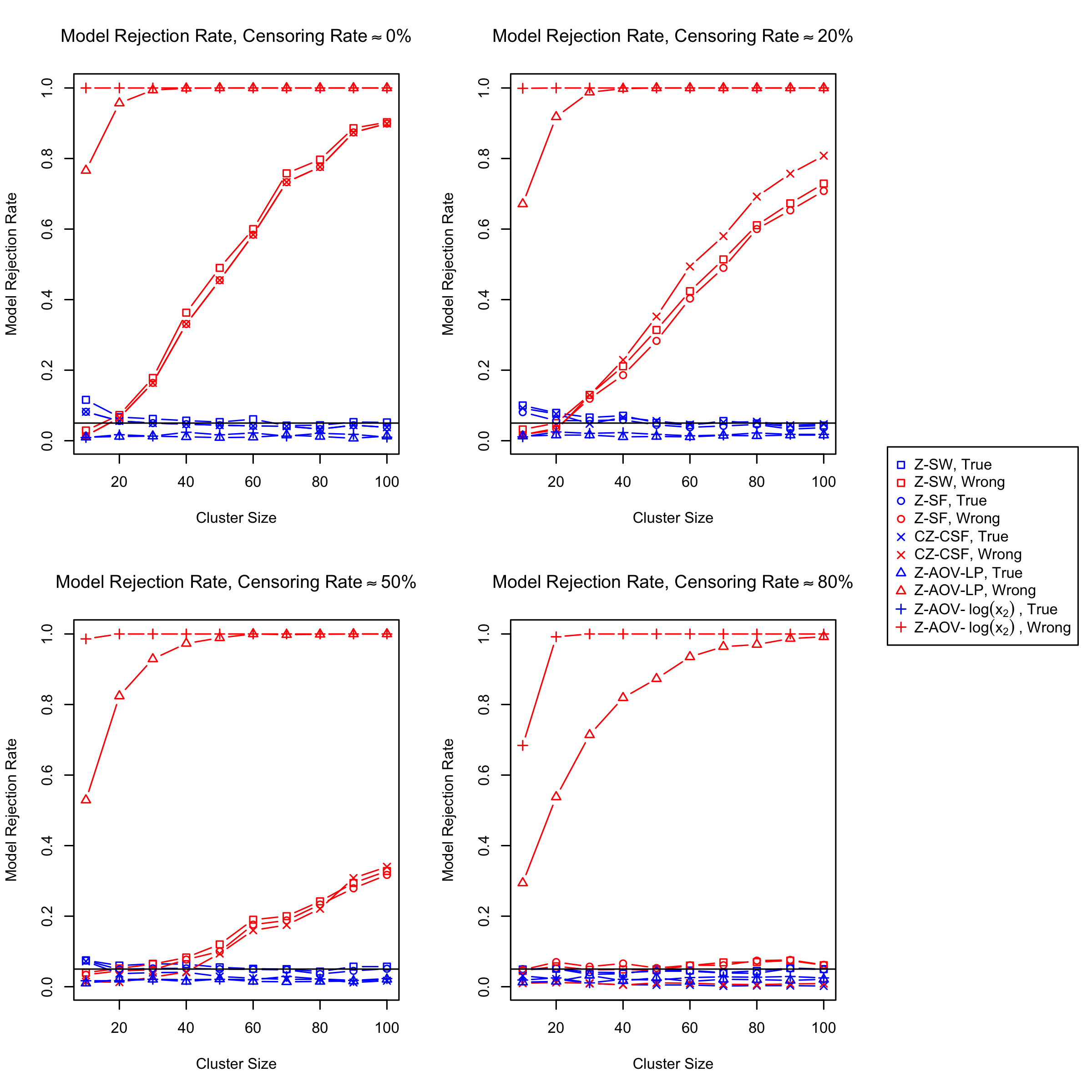
In addition to the graphical assessment, numerical tests with Z-residuals can be constructed as Z-residuals are approximately distributed as the standard normal under the true model. We compare a set of residual-based testing methods for detecting the inadequacy of fitted models. The overall GOF test methods are denoted by “R-T” with “R” denoting the residual name and “T” denoting the test method. For example, Z-SW is the test method that the normality of Z-residuals is tested with the SW test. In particular, CZ-CSF is the method that the normality of censored Z-residuals (shortened by CZ) is tested by an extended SF method for censored observations, which is implemented with gofTestCensored in the R package EnvStats. For detecting the misspecification in the covariate functional form, we can divide Z-residuals into groups by cutting the linear predictor or a covariate into equally-spaced intervals as shown by the boxplots of Figure 2. We can then test the homogeneity of Z-residuals across the groups. Z-AOV-LP is the method of applying ANOVA to test the equality of the means of Z-residuals against the groups formed with the linear predictor (LP) and Z-AOV- is the method of testing the equality of the means of Z-residuals against the groups formed with the covariate .
We simulated 1000 datasets for each combination of cluster size and censoring rate as described at the beginning of this section. Using the 1000 datasets generated from the true model under each scenario, the model rejection rate of each test method was estimated by the proportion of the test p-values less than 0.05. The model rejection rates of all the considered test methods are shown in Figures 4 and 7. The non-homogeneity test methods, Z-AOV-LP and Z-AOV-, can detect the non-linear covariate effects with very high true-positive rates (model rejection rates under the wrong models) and low false-positive rates (model rejection rates under the true models). Of all the compared test methods, Z-AOV- performs the best for detecting the nonlinear covariate effects with the highest powers, which are nearly 100%, and the powers stay high even for the scenario with a cluster size as small as 10. The Z-SW, Z-SF, and CZ-CSF tests have false-positive rates close to the nominal level of 5% for all scenarios and have certain powers when the censoring rate is less than 80%. We also note that their powers increase as the cluster size increases. However, the powers of these overall GOF tests are significantly smaller than the corresponding powers of the Z-AOV-LP and Z-AOV- methods. The comparison demonstrates the advantage of testing the homogeneity of Z-residuals for checking the assumption of covariate functional form in addition to the overall GOF tests, which do not inspect the relationship between residuals and covariates.
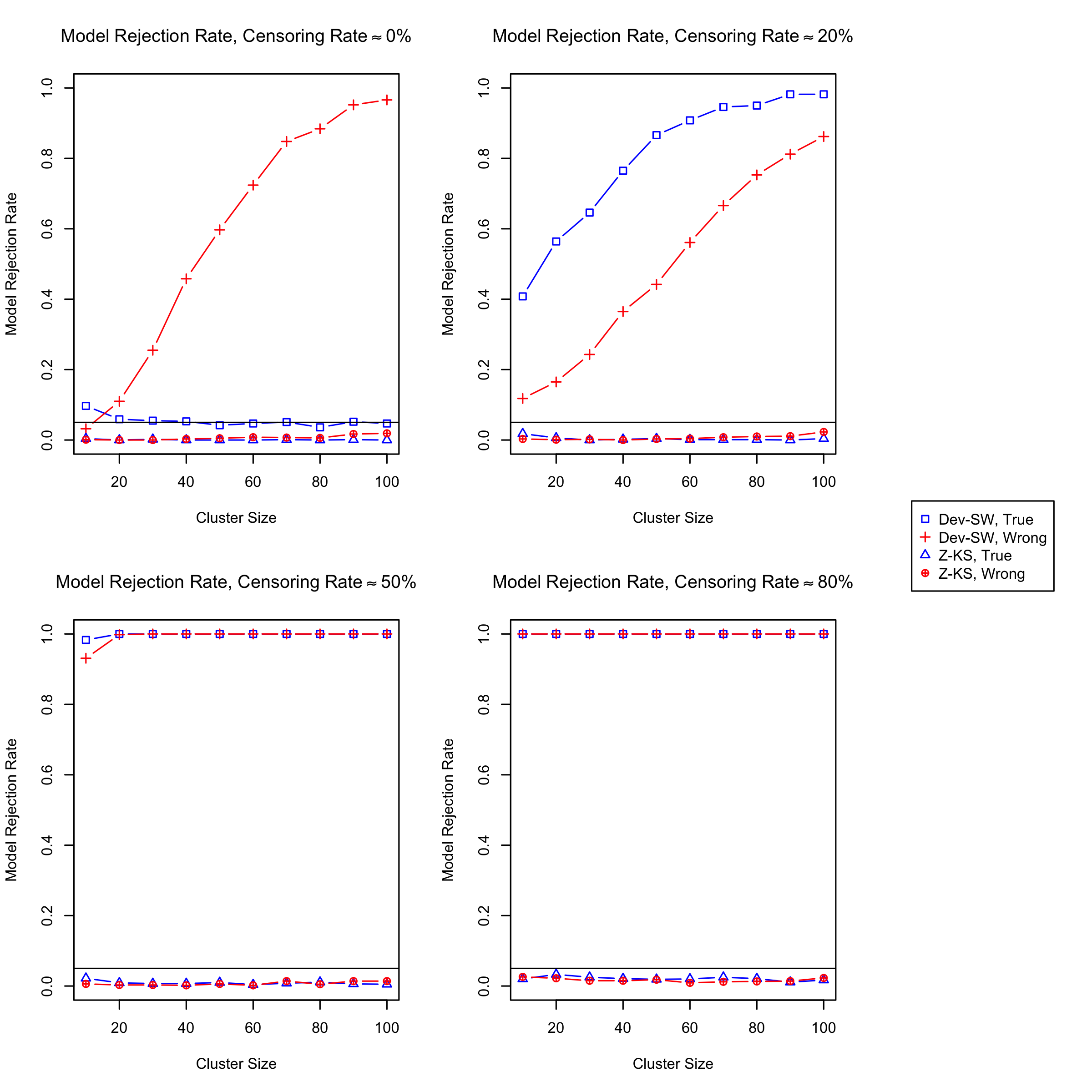
In appended Figure 7, we show the performances of the Z-KS and Dev-SW tests, which were separated from Figure 4 for better visualization. Z-KS test has low false-positive rates but also very low powers, which shows the conservatism of the KS test for testing the normality of Z-residuals. When the censorship is 0, the performance of Dev-SW is satisfactory. However, when there are censored observations, the Dev-SW method has very high (nearly 100%) model rejection rates when the model is correctly specified. Hence, the high powers of Dev-SW do not indicate that it is a good test method.
6 A Real Data Example
In this section, we apply the proposed residual diagnostics tools based on Z-residuals to diagnose the functional form of covariates in a real application for modelling the survival times of acute myeloid leukemia patients. The dataset contains 1498 patients recorded at the M. D. Anderson Cancer Center between 1980 and 1996 (Estey et al. 2000). The dataset used in our analysis contains 411 patients who are aged below 60 from 24 administrative districts recorded at the M.D Anderson Cancer Center between 1980 and 1996. The data collected information on the survival time for acute myeloid leukemia and prognostic factors, including age, sex, white blood cell count (wbc) at diagnosis, and the townsend score (tpi) for which higher values indicate less affluent areas. The censoring rate is 29.2%. The response variable of interest is the survival time in days, which is the time from entry to the study or death. The preliminary study showed that the wbc is highly right-skewed. Logarithm transformation is often used to reduce the impact of extremely large values of the covariate on the response variable, such as the wbc variable in this application. However, a logarithm transformation may mask the impact of extremely large values of the covariate on the outcome variable.
We fitted two shared frailty models, one with covariates wbc, age, sex and tpi, which is labelled as the wbc model, and the other with log(wbc) replacing wbc, which is labelled as the lwbc model. Table 1 shows the estimated regression coefficients, the corresponding standard errors and p-values for the covariate effects from fitting the two shared frailty models. The results indicate that the estimated effect of wbc is statistically significant (p-value 0.001) but the effect of log(wbc) is not significant (p-value=0.135). The difference in the p-values for wbc and log(wbc) highlights that the statistical inference of the covariate effect may depend on the assumption of the functional form of the covariates.
| Covariates | Estimate | SE | P-value |
|---|---|---|---|
| 0.021 | 0.005 | 0.000 | |
| 0.215 | 0.118 | 0.068 | |
| 0.005 | 0.001 | 0.000 | |
| 0.023 | 0.016 | 0.140 | |
| 0.906 |
| Covariates | Estimate | SE | P-value |
|---|---|---|---|
| 0.021 | 0.005 | 0.000 | |
| 0.216 | 0.118 | 0.069 | |
| 0.035 | 0.024 | 0.135 | |
| 0.024 | 0.016 | 0.128 | |
| 0.906 |
The overall GOF tests and graphical checking with CS residuals and Z-residuals show that both the wbc and lwbc models provide adequate fits to the dataset. The first row of Figure 5 shows that the estimated CHFs of the CS residuals of both of the wbc and lwbc models align closely along the diagonal line. Similarly, the QQ plots (the second row of Figure 5) of Z-residuals of these two models align well with the 45∘ diagonal line. The scatterplots of Z-residuals against the linear predictor don’t exhibit visible trends; their LOWESS lines are very close to the horizontal line at 0; the boxplots of Z-residuals grouped by cutting linear predictors into equal-spaced intervals (the fourth row of Figure 5) appear to have equal means and variance across groups. The Z-AOV-LP test also gives large p-values for the wbc and lwbc models (0.63 and 0.76 respectively).
The above diagnostics results reveal no serious misspecification in these two models. However, the inspection of the Z-residuals against the covariate log(wbc) reveals that the functional form of the lwbc model is likely misspecified. The scatterplots and comparative boxplots of the Z-residuals against log(wbc) are shown in the fifth and sixth rows of Figure 5. The LOWESS curve of the wbc model appears to align well with the horizontal line at 0 and the grouped Z-residuals of the wbc model appear to have equal means and variances across groups. However, the diagnosis results for the lwbc model are very different. It appears that there is a non-linear trend in the LOWESS curve of the lwbc model and the grouped Z-residuals appear to have different means across groups. To measure the statistical significance of the observed trends, we apply Z-AOV- to test the equality of the means of the grouped Z-residuals of these two models. The p-values are 0.16 and 0.00 respectively for the wbc and lwbc models as shown in the boxplots. The very small p-value of the Z-AOV-log(wbc) test for the lwbc models strongly suggests that the log transformation of wbc is likely inappropriate for modelling the survival time.
The Z-residual test p-values quoted above contain randomness because of the randomization in generating Z-residuals. To ensure the robustness of the model diagnostics results, we generated 1000 replicated test p-values with 1000 sets of regenerated Z-residuals for each test method. Figure 6 displays the histograms of 1000 replicated Z-residual test p-values for the wbc and lwbc models. The red vertical lines in these histograms show the upper bound summaries of these replicated p-values, (see Sec. 4.3 for details). These histograms show that the Z-SW, Z-SF, and Z-AOV-LP tests for both models give a large proportion of p-values greater than 0.05, and the large p-values result in large values. In contrast, the replicated Z-AOV-log(wbc) p-values for the lwbc model are almost all smaller than 0.001. The consistently small Z-AOV-log(wbc) p-values further confirm that the log transformation of wbc is inappropriate for modelling the survival time.
Table 2 tabulates all the values (shown with red lines in Figure 6) for diagnosing the two models with Z-residual-based tests. In addition, we also report the non-random CZ-CSF test p-values for the two models and the AIC values for comparing these two models. The CZ-CSF p-values of both models are larger than 5% (Table 2). Therefore, the CZ-CSF test does not identify the inadequacy of the lwbc model either. The AIC value, 3132.105, of the lwbc model, is much larger than the AIC value 3111.669 of the wbc model, which indicates that the wbc model provides a better model fit compared to the lwbc model. This conclusion is consistent with the model diagnostics results as given by the Z-AOV-log(wbc) test, which reveals that the lwbc model is inappropriate for modelling the survival time of this dataset by checking the homogeneity of Z-residuals against log(wbc). Although the AIC of the wbc model is smaller than that of the lwbc model, we also see that a large proportion of Z-AOV-log(wbc) p-values for the wbc model are tiny; the value is 0.074. We think that the wbc model could be improved to provide a better fit for the survival time of this dataset.
| Model | AIC | CZ-CSF | Z-SW | Z-SF | Z-AOV-LP | Z-AOV-log(wbc) |
|---|---|---|---|---|---|---|
| value | ||||||
| wbc model | 3111.669 | 0.255 | 0.495 | 0.693 | 0.703 | 0.074 |
| lwbc model | 3132.105 | 0.305 | 0.579 | 0.781 | 0.978 | 0.00001 |
7 Conclusions and Discussions
In this paper, we extended the idea of randomized survival probability (Li et al. 2021) to develop a residual diagnostic tool that can provide both graphical and numerical results for checking the covariate functional form in semi-parametric shared frailty models. We proposed a non-homogeneity test for testing whether there is a trend in Z-residuals for checking the covariate functional form. Our extensive simulation studies showed that the overall GOF tests (including CS-CSF, Z-SW, and Z-SF) may not be powerful enough for detecting the misspecification in covariate functional form and that the proposed non-homogeneity tests based on the Z-residuals are significantly more powerful than the aforementioned overall GOF tests. Applied to a real dataset, the Z-residual diagnostics discovers that a model with log-transformation is inappropriate for modelling the survival time of acute myeloid leukemia patients, which is not captured by other diagnostics methods.
The Z-residuals-based diagnostics methods can be extended in several directions. When the full dataset is used to estimate the model parameters and used to calculate residuals for model checking, there might be a conservatism problem (bias) due to the double use of the dataset. The double use of the data may reduce the power of detecting model misspecification, especially in the case of small sample size or high censoring rate. Cross-validation could be a good method to solve this problem. The cross-validatory Z-residual may be a more powerful tool for identifying the model inadequacy in the survival data.
In this paper, we considered semiparametric shared frailty models assuming proportional hazards. However, if the model includes time-varying coefficients or time-dependent explanatory variables, the proportional hazards assumption may be violated. A number of residuals have been proposed for evaluating the assumption of proportional hazards. Traditionally, the Schoenfeld (Collett 2015; Schoenfeld 1982) and Scaled Schoenfeld (Grambsch and Therneau 1994) residuals are often used in testing the assumption of proportional hazard. Lin et al. 1993 proposed the cumulative sums of martingale residuals to check the validity of the PH assumption. Extending the Z-residual for diagnosing the proportional hazard assumption and comparing it with existing residual diagnostics tools warrants a research topic in the future.
Appendix A Additional Figures and Tables
References
- Balan and Putter (2020) Balan TA and Putter H (2020) A tutorial on frailty models. Statistical Methods in Medical Research 29(11): 3424–3454.
- Caraux and Gascuel (1992) Caraux G and Gascuel O (1992) Bounds on distribution functions of order statistics for dependent variates. Statistics & Probability Letters 14(2): 103–105.
- Clayton (1978) Clayton DG (1978) A Model for Association in Bivariate Life Tables and Its Application in Epidemiological Studies of Familial Tendency in Chronic Disease Incidence. Biometrika 65: 141–151.
- Collett (2015) Collett D (2015) Modelling Survival Data in Medical Research. Chapman and Hall/CRC.
- Cox (1972) Cox DR (1972) Regression models and life-tables. Journal of the Royal Statistical Society. Series B, Methodological 34(2): 187–220.
- Cox and Snell (1968) Cox DR and Snell EJ (1968) A general definition of residuals. Journal of the Royal Statistical Society. Series B (Statistical Methodology) 30(2): 248–275.
- Davison and Gigli (1989) Davison AC and Gigli A (1989) Deviance residuals and normal scores plots. Biometrika 76(2): 211–221.
- Downton (1972) Downton F (1972) Discussion on Professor Cox’s Paper. Journal of the Royal Statistical Society. Series B, Methodological 34(2): 202–220.
- Duchateau and Janssen (2004) Duchateau L and Janssen P (2004) Penalized Partial Likelihood for Frailties and Smoothing Splines in Time to First Insemination Models for Dairy Cows. Biometrics 60(3): 608–614.
- Duchateau and Janssen (2008) Duchateau L and Janssen P (2008) The Frailty Model. Statistics for Biology and Health. New York: Springer Verlag. ISBN 978-0-387-72834-6.
- Estey et al. (2000) Estey EH, Shen Y and Thall PF (2000) Effect of time to complete remission on subsequent survival and disease-free survival time in AML, RAEB-t, and RAEB. Blood 95(1): 72–77.
- Farrington (2000) Farrington CP (2000) Residuals for proportional hazards models with interval-censored survival data. Biometrics 56(2): 473–482.
- Grambsch and Therneau (1994) Grambsch PM and Therneau TM (1994) Proportional hazards tests and diagnostics based on weighted residuals. Biometrika 81(3): 515–526.
- Hanagal (2015) Hanagal D (2015) Modeling survival data using frailty models. Statistical methods in Medical Research 24(6): 936–936.
- Henderson et al. (2002) Henderson R, Shimakura S and Gorst D (2002) Modeling spatial variation in leukemia survival data. Journal of the American Statistical Association 97(460): 965–972.
- Hillis (1995) Hillis SL (1995) Residual plots for the censored data linear regression model. Statistics in Medicine 14(18): 2023–2036.
- Hougaard (1995) Hougaard P (1995) Frailty models for survival data. Lifetime Data Analysis 1(3): 255–273.
- Hougaard (2000) Hougaard P (2000) Analysis of Multivariate Survival Data. Springer.
- Kaplan and Meier (1958) Kaplan EL and Meier P (1958) Nonparametric estimation from incomplete observations. Journal of the American Statistical Association 53(282): 457–481.
- Karagrigoriou (2011) Karagrigoriou A (2011) Frailty models in survival analysis. Journal of Applied Statistics 38(12): 2988–2989.
- Keleş and Segal (2002) Keleş S and Segal MR (2002) Residual-based tree-structured survival analysis. Statistics in Medicine 21(2): 313–326.
- Law and Jackson (2017) Law M and Jackson D (2017) Residual plots for linear regression models with censored outcome data: A refined method for visualizing residual uncertainty. Communications in Statistics - Simulation and Computation 46(4): 3159–3171.
- Li et al. (2021) Li L, Wu T and Feng C (2021) Model diagnostics for censored regression via randomized survival probabilities. Statistics in Medicine 40(6): 1482–1497.
- Lin (2007) Lin DY (2007) On the Breslow estimator. Lifetime Data Analysis 13(4): 471–480.
- Lin et al. (1993) Lin DY, Wei LJ and Ying Z (1993) Checking the Cox Model with Cumulative Sums of Martingale-Based Residuals. Biometrika 80(3): 557–572.
- Lin et al. (1998) Lin DY, Wei LJ and Ying Z (1998) Accelerated failure time models for counting processes. Biometrika 85(3): 605–618.
- McCullagh and Nelder (1989) McCullagh P and Nelder JA (1989) Generalized Linear Models, Second Edition. CRC Press. ISBN 978-0-412-31760-6.
- McGilchrist (1993) McGilchrist CA (1993) REML Estimation for Survival Models with Frailty. Biometrics 49(1): 221.
- Millard (2018) Millard SP (2018) EnvStats: Package for Environmental Statistics, Including US EPA Guidance.
- Nardi and Schemper (1999) Nardi A and Schemper M (1999) New Residuals for Cox Regression and Their Application to Outlier Screening. Biometrics 55(2): 523–529.
- Peng and Taylor (2017) Peng Y and Taylor JMG (2017) Residual-based model diagnosis methods for mixture cure models. Biometrics 73(2): 495–505.
- Ripatti and Palmgren (2000) Ripatti S and Palmgren J (2000) Estimation of Multivariate Frailty Models Using Penalized Partial Likelihood. Biometrics 56(4): 1016–1022.
- Rychlik (1992) Rychlik T (1992) Stochastically extremal distributions of order statistics for dependent samples. Statistics & probability letters 13(5): 337–341.
- Schoenfeld (1982) Schoenfeld D (1982) Partial residuals for the proportional hazards regression model. Biometrika 69(1): 239–241.
- Shepherd et al. (2016) Shepherd BE, Li C and Liu Q (2016) Probability-scale residuals for continuous, discrete, and censored data. The Canadian journal of statistics = Revue canadienne de statistique 44(4): 463–479. 10.1002/cjs.11302.
- Steven P. Millard (2013) Steven P Millard (2013) EnvStats: An R Package for Environmental Statistics. 2nd ed. 2013.. edition. New York, NY: Springer. ISBN 978-1-4614-8456-1.
- Therneau (2022) Therneau TM (2022) A Package for Survival Analysis in R. URL https://CRAN.R-project.org/package=survival. R package version 3.3-1.
- Therneau and Grambsch (2013) Therneau TM and Grambsch PM (2013) Modeling Survival Data: Extending the Cox Model. Springer Science & Business Media.
- Therneau et al. (1990) Therneau TM, Grambsch PM and Fleming TR (1990) Martingale-based residuals for survival models. Biometrika 77(1): 147–160.
- Vaupel et al. (1979) Vaupel JW, Manton KG and Stallard E (1979) The impact of heterogeneity in individual frailty on the dynamics of mortality. Demography 16(3): 439–454.
- Yuan and Johnson (2012) Yuan Y and Johnson VE (2012) Goodness-of-Fit Diagnostics for Bayesian Hierarchical Models. Biometrics 68(1): 156–164.