All plus four point (A)dS graviton function using generalized on-shell recursion relation
Abstract
This paper presents a calculation of the four gravitons amplitude in (Anti)-de Sitter space, focusing specifically on external gravitons with positive helicity. To achieve this, we employ a generalized recursion method that involves complexifying all external momentum of the graviton function, which results in the factorization of AdS graviton amplitudes and eliminates the need for Feynman-Witten diagrams. Our calculations were conducted in three boundary dimensions, with a particular emphasis on exploring cosmology and aiding the cosmological bootstrap program. To compute the expression, we utilized the three-dimensional spinor helicity formalism. The final expression was obtained by summing over residues of physical poles, and we present both symbolic and numerical results. Additionally, we discuss the advantages and limitations of this approach, and highlight potential opportunities for future research.
I Introduction
The surprising simplicity of scattering amplitudes in flat space has provided a beautiful conundrum: why is the scattering amplitudes of gravity simple, given the non-linear nature of general relativity? Attempts to understand this underlying elegance has driven important advancements in theoretical physics in recent years Elvang:2013cua. One of the most effective tools for studying the simplicity of these observables in flat space is the on-shell recursion relations, which express the scattering amplitudes of higher point amplitudes as a sum of products of lower-point amplitudes Britto:2005fq.
Alongside the advances in Minkowski space, there has been a growing emphasis on the study of holographic observables. Holography finds concrete appearance in asymptotically Anti-de Sitter (AdS) spacetimes, where AdS scattering amplitudes are equivalent to the correlation functions of a conformal field theory (CFT) on the boundary Maldacena:1997re. Many innovative techniques such as Mellin space, conformal bootstrap, and harmonic analysis in AdS are used in the computations of these correlators Penedones:2010ue; Fitzpatrick:2011ia; Rastelli:2016nze; Heemskerk:2009pn; Costa:2014kfa; Sleight:2017fpc; Fitzpatrick:2011dm; Costa:2014kfa; Paulos:2011ie; Kharel:2013mka. This work will build upon progresses made in (A)dS momentum space Bzowski:2013sza; Bzowski:2015pba; Bzowski:2018fql; Bzowski:2015pba; Bzowski:2019kwd; Bzowski:2020kfw; Isono:2018rrb; Isono:2019wex; Coriano:2013jba; Coriano:2018bbe; Anand:2019lkt; Farrow:2018yni; Nagaraj:2019zmk; Nagaraj:2020sji; Jain:2020rmw; Meltzer:2020qbr; Albayrak:2018tam; Albayrak:2019asr; Albayrak:2019yve; Albayrak:2020isk; Albayrak:2020bso; Bzowski:2022rlz; Caloro:2022zuy; Meltzer:2021zin. However, we use an approach which has been largely under-used in curved spacetime. Instead of relying on perturbative Feynman-Witten diagrams, we will use recursion relations to compute our expression, revisiting an attractive perspective on the topic that was started in these seminal papers Raju:2012zr; Raju:2012zs.
A compelling reason to investigate these correlators in momentum space is due to its close relationship to the wave function of the universe Maldacena:2002vr; Ghosh:2014kba. Therefore, the cosmological bootstrap Arkani-Hamed:2018kmz; Baumann:2019oyu; Baumann:2020dch; Sleight:2019hfp; Sleight:2020obc and cosmological collider physics programs Arkani-Hamed:2015bza; Wang:2022eop; Niu:2022fki; Niu:2022quw; Xianyu:2022jwk; Qin:2022lva; Reece:2022soh; Reece:2022soh; Heckelbacher:2022hbq; Pinol:2021aun; Lu:2021wxu; DiPietro:2021sjt; Kumar:2019ebj; Hook:2019vcn; Hook:2019zxa; Alexander:2019vtb; Aoki:2023tjm; Qin:2023ejc; Pimentel:2022fsc; Tong:2022cdz; Baumann:2019ztm have been putting an organized effort to unravel the properties of cosmologically relevant correlators. While the language of AdS computations looks different, the techniques here translate naturally to cosmology as both AdS and cosmological correlators exhibit a total energy singularity when sum of the norms of the momenta are analytically continued to zero. The behavior of the correlator around this singularity is closely linked to the scattering amplitude for the same process in flat space, meaning that holographic and cosmological correlators contain within them valuable physics of the flat space scattering amplitudes.
In curved spaces, on-shell recursion relations require various modifications,11 1 Firstly, it is not a priori given that a correlator in general curved spaces is a meromorphic function, hence the usual contour-deformation arguments of BCFW needs to be altered to take into account the other singularities. Secondly, the absence of the conservation of momentum along the bulk direction complicates the deformation. Luckily, flat-space-like on-shell recursion relations do exist in (A)dS, and one can work with a simple deformation by sticking to momentum space in the Poincaré patch as we detail in the body. which is especially true for the three-dimensional boundaries that are most relevant to cosmology. In three dimensions, the standard two-line shift used in BCFW recursion relations is not possible, so a generalization to an -line deformation is necessary Raju:2012zs. However, this significantly increases the number of partitions to consider, which reduces efficiency. Moreover, the complexity of the computation is further increased by the fact that the deformation parameter satisfies a quadratic equation, as the boundary momenta are not null. These challenges have hindered the use of RBCFW (Raju’s extension of BCFW in AdS), developed by Raju over a decade ago. In our work, we aim to clarify these challenges and demonstrate the areas where (A)dS on-shell methods are most effective.
Our paper aims to calculate the four point graviton amplitude with all plus external helicities using RBCFW and spinor helicity techniques. There have been other recent approaches to this problem where the authors compute late time four point function and the related quartic coefficient by direct computation and by other approaches Bonifacio:2022vwa. Similarly, authors of this paper have computed up to five point exchange diagrams in AdS in Albayrak:2019yve. However, we will proceed with RBCFW instead, and compute four point all plus helicity graviton amplitude. Besides being previously uncomputed, all plus helicity has also been historically important in the flat space scattering amplitude program as a playground to discover structures about more complicated amplitudes. Interestingly, the four point flat space all plus helicity amplitude vanishes at tree-level; but for pure Yang-Mills and gravity, the loop level counterpart is non-zero for non-supersymmetric cases. These amplitudes have been used as toy examples to study non-supersymmetric amplitudes in flat space. Nevertheless, the task to compute this function in (A)dS for graviton is rather formidable. It’s important to remember that even in flat space, computing the four point graviton amplitude is a challenging task that was only made easier with the development of on-shell recursion techniques. However, in principle, using RBCFW is a straightforward approach to tackle these calculations. Moreover, recursive methods can be employed to compute higher point amplitudes without having to worry about the infinite series of interaction vertices that arise from the expansion of the Einstein-Hilbert action. Therefore, we believe that this is an intriguing approach that demands more attention.
The paper is structured as follows. In § II, we briefly review the momentum space perturbation theory and on-shell methods in AdS via providing the necessary ingredients for the calculations. In § III, we compute the all plus helicity four point graviton amplitude and analyze it from different analytical and numerical perspectives. We then conclude in § IV by discussing the efficacy of RBCFW computations as to the weaknesses and strengths of this technology. In particular, we detail in what kind of computations we believe that this method would shine, and then close with an outlook. We collect the technical details in the appendix, along with a review of the spinor helicty formalism in AdS.22 2 The attached Mathematica files contain the less presentable data, such as the symbolic expression for the full amplitude and the data points for Figure 1.
II Preliminaries
II.1 Momentum space perturbation theory in AdS
We start by setting our conventions and notations. We work in Poincaré coordinates with the metric : is the radial coordinate, approach the boundary as , and is the boundary metric in mostly positive signature. As we preserve the manifest translation symmetry at the boundary, we will make use of it by going to the boundary Fourier domain and working with the coordinates , following the treatment of the related papers in the literature Raju:2010by; Raju:2011mp; Raju:2012zs; Raju:2012zr; Albayrak:2018tam; Albayrak:2019asr; Albayrak:2019yve; Albayrak:2020isk; Albayrak:2020bso; Albayrak:2020fyp.
The perturbative treatment of gravity in AdS is relatively complicated albeit straightforward:33 3 The quadratic part of the gravity action can be used to obtain the bulk to bulk propagator, from which one can obtain the bulk to boundary propagator by taking one of the vertices to the boundary. we will simplify the expressions by sticking to the axial gauge, i.e. . In this gauge, the bulk-to-boundary propagator reads as
| (2.1a) | ||||
| whereas the bulk to bulk propagator is | ||||
| (2.1b) | ||||
Here, denote the norm of , is the polarization vector, and the tensor is defined as . Finally, the vertex factor for the graviton cubic self-interaction is44 4 Note the contravariant form for the vertex factor (hence ).
| (2.2) |
We refer the reader to Raju:2011mp for further details on the derivation of these ingredients.
The computation of Witten diagrams in this formalism is quite straightforward: we take the contracted product of necessary ingredients and then integrate over bulk radius of internal vertices; for instance, the three point graviton amplitude has the expression
| (2.3) |
The Witten diagrams computed along these lines correspond to the vacuum correlators with all sources in the same Poincaré patch. In contrast, general correlation functions in global AdS may have sources in multiple patches; when viewed from one patch, insertions in the other patches are invisible and they simply amount to creating boundary conditions on the past and future horizons of the chosen patch Raju:2011mp. Such objects are called transition amplitudes, and we can derive them from the usual Witten diagrams by a simple replacement of bulk to boundary propagators (corresponding to the insertions in the other patches) with normalizable modes: in practice, this is equivalent to the replacement of the modified Bessel function of the second kind () with the Bessel function of the first kind (). In this paper, we will only need two transition amplitudes:
| (2.4a) | ||||
| (2.4b) | ||||
which can be straightforwardly derived as is done in Raju:2012zs.55 5 are “scalar” parts of the transition amplitudes that depend only on the norms of the vectors; see eqn. (A.9) for their explicit expressions. The brackets refer to the products of spinor-helicities: we review our spinor helicity conventions in § A.1.
II.2 Recursion relations in AdS
In this section, we will briefly review the recursion relations introduced in Raju:2012zr, which generalizes the previous work of the author Raju:2010by; Raju:2011mp in AdS and Risager’s work in flat space Risager:2005vk.
Our starting point is the observation that we have
| (2.5) |
where parameterizes the external legs and is a judiciously chosen set. This equality follows from the linear dependence of vectors for sufficiently high :66 6 In low dimensions, such as (AdS4), this is evidently true for four and higher point amplitudes. In higher dimensions, one can still proceed by decomposing the general polarization vector to a linear sum of special ones for which this equation is true, see §4.4 of Raju:2011mp. it allows the deformation of the external momenta while still preserving the momentum conservation:
| (2.6) |
One can go ahead and use a contour deformation in the plane to rewrite any tensor in terms of its residues along with a possible boundary contribution. In the cause of gauge and gravity correlators, the Ward identities actually help us constraint the possible form of the boundary term; in the end, one is left with the following recursion relation:
| (2.7) |
where is a boundary term and is a bi-partitioning of the set into the sets and such that . The piece can be reconstructed from lower-point transition amplitudes as
| (2.8) |
for
| (2.9) |
where is a transition amplitude in the sense that it is same with upto the replacement of the bulk-to-boundary propagator of the momentum--particle with a normalizable mode. The momentum is defined as
| (2.10) |
where are solutions to the constraint .
The algorithm of obtaining a higher point amplitude from a lower one is therefore:
- 1.
Turn lower point amplitude to a transition amplitude by replacing one of the bulk-to-boundary propagators with a normalizable mode
- 2.
Glue two such transition amplitudes, fixing the momentum of internal leg by eqn. (2.10)
- 3.
Solve for : this is precisely what differentiates the curved space from the flat one as this relation is quadratic, unlike the linear relation of standard BCFW.
- 4.
Compute via eqn. (2.8). We will focus on AdS4, for which the relation will turn into an equality with a proportionality constant for the stress tensor correlator.77 7 See eqn. (4.12) of Raju:2012zs for the more general case.
- 5.
Sum over all possible permissable bi-partitions: this gives the integrand of higher point amplitude up to a constrained boundary piece.88 8 The boundary piece is of the form (2.11) for rational functions , where the second piece cancels the divergent part of .
- 6.
Do the integration in eqn. (2.7). The integrand will be even in for all cases in this paper, therefore we can convert the integral into a residue integration where the contribution at the infinity is canceled precisely by the boundary piece .
III Four point graviton amplitude in AdS4
III.1 Derivation of the general result
We start by considering the polarization sum of the product of transitional amplitudes in the bi-partition . By using the identity eqn. (A.10) and some massaging, we get
| (3.1) | ||||
where stands for the internal leg, and where and the operator are defined in the Appendix A.2.
As shown in eqn. (2.9), we actually need to deform the spinors as induced by the deformation of in eqn. (2.6);99 9 We are considering all-line deformation, hence the set is . in our case, this amounts to shifting the spinor as
| (3.2) |
for given in eqn. (A.21), where external ’s remain the same. Thus, we only need to apply the deformation of the internal ,1010 10 We use the identities (3.3a) (3.3b) derived in Raju:2012zs. which leads to
| (3.4) |
where we denote the deformed spinors by a superscript for brevity, i.e. and so on.
Alternatively, we could use momentum conservation to get rid of the explicit dependence on the internal leg first:1111 11 In spinors, reads as (3.5) which is used twice: first to rewrite as , second to remove internal spinor completely. this leads to an expression with explicit ’s (not just ’s as eqn. (3.1)), which deforms nontrivially to the final form
| (3.6) |
We will make use of this alternative (yet equivalent) form below; nevertheless, let us proceed for now with the former expression. Inserting it into eqn. (2.8), we get
| (3.7) |
where we used eqn. (A.17) to pull to the leftmost and set .1212 12 This is consistent both with normalizable mod having a negative imaginary part required by the correct analytical continuation Raju:2012zr, and with the constraint in the recursion prescription.
As we are interested in all plus helicity amplitude, different bi-partitions can be straightforwardly related to each other via ; in fact, by using eqn. (A.16) and eqn. (A.17), we can immediately write down in the form . All that is left is to insert this in eqn. (2.7), which turns into a simple residue extraction as explained in the final item of the algorithm above; thus, putting everything together, we arrive at the final expression
| (3.8) |
where we define
| (3.9) |
for brevity, e.g. .
One can compute the residues and insert the computed in Appendix A.3; to illustrate, let us consider the last residue. After a manageable calculation,1313 13 Although these computations are straightforward –albeit tediously long, we streamlined them like the rest of the calculations in this paper via the proprietary software Mathematica and the handy packages xAct & xTensor garcia:2004xact; garcia:2004xtensor. one can show that the brackets at that residue satisfy
| (3.10a) | ||||
| (3.10b) | ||||
| (3.10c) | ||||
which yields the result
| (3.11) |
for . The other residues can be computed analogously: the full explicit result can be found in the attached Mathematica file.
III.2 Center of mass frame
The general result in eqn. (3.8) can be written in a simpler form by boosting to the center of mass frame, i.e. .1414 14 We do not lose any generality here as this is an invertible transformation. The identity for ensures
| (3.12) |
in this frame, which simplify the overall computation. In particular, partition gets the rather nice form
| (3.13) |
for defined in eqn. (A.25), where the only dependence is carried by the following coefficients
| (3.14) |
Despite not being in a polynomial form in , the other partitions are still simpler in this frame, e.g.
| (3.15) |
where are known combinations of square and angle brackets, given in eqn. (A.26).
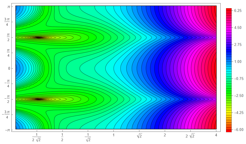
III.3 Overall behavior of the amplitude
In the previous section, we introduced the center of mass frame in which the amplitude takes a simpler form. We can further fix the configuration such that1515 15 By starting in a generic coordinate system, one can arrive at this configuration by (1) boosting to the center of mass frame, (2) scaling the zeroth coordinate so that , (3) shifting the zeroth coordinate so that , (4) rotating the other coordinates so that . As all of these transformations are invertible, the whole process amounts to fixing the symmetry without losing generality.
| (3.16) | ||||
where is the angle between the vectors and ,1616 16 Mathematically speaking, the actual angle between the vectors and is ; however, we will refer to as the angle as it measures the collinearity of and in the spatial coordinates. and is the ratio of the norms and . In this frame, we have
| (3.17) |
where we can explicitly compute ; for instance, the piece in front of becomes
| (3.18) |
However, the other pieces are more complicated and it is in fact not sensible to consider individual pieces as they develop spurious poles in this frame.1717 17 We physically expect (and numerically verify) that the full amplitude does not have poles at the locations and ; hence we know the singularities in the individual contributions to be spurious. Therefore, we consider the full amplitude instead, and extract its overall behavior with respect to its arguments numerically, which we present in Figure (1). We provide the corresponding data in the attached Mathematica file.
IV Conclusions
In this paper, we symbolically computed the four point graviton amplitude in AdS for all plus external helicities. We did this by using the AdS on-shell recursion relations, which have seen limited attention and have not been used in explicit full computations since their introduction more than a decade ago.1818 18 At the same time of his introduction of this technology in Raju:2012zr, the author publishes another paper in which he actually carries out explicit computation of four point graviton amplitude of helicities Raju:2012zs. However, that computation does not fairly represent the technical difficulty of this technology, because most of the partitions for (and only for) this set of helicities have deformations free of square roots (main complication of quadratic solution for deformation). As we mentioned in the introduction, on-shell recursion relations in curved spaces are far more complicated than their flat space counterparts, and this work is intended to serve the goal of being a playground to test the strengths and weaknesses of BCFW on AdS.
We found out that RBCFW is rather efficient at providing compact implicit results, as we did with eqn. (3.8). Indeed, we were able to package the formidable four point graviton amplitude in AdS to mere four lines without the use of any four point interaction vertices. However, to get the full explicit result, one needs to extract out the deformations (see eqn. (3.10)) and compute the residues, which are straightforward albeit tedious computations. One still needs to take these residues in the usual diagrammatic approach, since Witten diagrams also have analogous bulk integrals; nevertheless, the deformation itself is rather lengthy in the general case as we detail in § A.3. However, all of the necessary steps are highly algorithmic, which takes us to our next point.
We have observed that the rigid algorithmic approach in RBCFW (as loosely listed at the end of § II) makes it rather straightforward to implement the calculations into a symbolic computation software. Indeed, we wrote a short script in the propriety program Mathematica to carry out the computations: this allowed us to obtain the full, explicit result, which we provide in the attached file. The downside though is that the result is not yet in the shortest possible form,1919 19 It is relatively hard to teach Mathematica to make use of all Schouten identities and momentum conservations in an intelligent and time-efficient way; perhaps the machine learning can be utilized for such optimization tasks in future. which makes it improbable to extract a physical intuition.
Besides computing the amplitude, we also commented with explicit results on how certain configurations simplify the calculations; nevertheless, they are still too lengthy to be performed by pen and paper. We believe that certain limits should make them more manageable, and we plan to explore this in our next project. It is of course plausible as well to compute higher point amplitudes and see how the complexity of explicit results change with that. Furthermore, one could introduce machine learning or more general AI tools to explore various ways to train the software to simplify the lengthy results into forms from which clearer physical intuitions can be extracted. Additionally, it is entirely possible that using the right variable rather than the three dimensional spinor helicity might be the best way to move forward: we believe that more attention needs to go into the investigation of the right variables to approach this problem.
These points aside, we do see some simplicity. Much like in Raju’s work, perhaps the most physical pole coming from the propagator in the four point diagrams yields the simplest result, leading to cancellation of all the messy terms. However, we still need to understand how best to simplify the expressions coming from the poles of the lower point amplitudes. In summary, on-shell recursion relations in AdS can really be useful to get the full explicit results in a reliable and fast fashion, without caring for the redundancies in the result.2020 20 As noted before, our current implementation does not make much use of various identities. They are also quite useful to compute numerical results, which are valuable data to compare with experiments. These advantages become radically more significant in the calculation of higher point amplitudes since the approach is sufficiently robust and efficiently recursive. Additionally, they could be a useful device to check double copy relations for higher point amplitudes in (A)dS Lee:2022fgr; Li:2022tby; Drummond:2022dxd; Herderschee:2022ntr; Sivaramakrishnan:2021srm; Diwakar:2021juk; Zhou:2021gnu; Albayrak:2020fyp; Armstrong:2020woi.
Before closing, we will share a poignant anecdote from DeWitt.2121 21 We were inspired to mention this historical allegory after coming across a similar and uplifting tale in a related paper, where we found a quote from Parke and Taylor on page 39 Bonifacio:2022vwa. In 1968, Bryce DeWitt impressively computed the four-point scattering amplitudes for gravitons DeWitt:1967uc. In the paper, DeWitt writes a sagacious commentary on the subject that remains striking to this day. He says, “it is a pity that nature displays such indifference to so intriguing and beautiful a subject [graviton scattering], for the calculations themselves are of considerable intrinsic interest.” DeWitt later says “there must be an easier way” due to the significant amount of cancellation between terms. Despite the fact that this quote has been partially buried in the passage of time, posterity has ultimately vindicated his belief, about the simplicity of these structures, to be correct. Admittedly, in modern times, we have at our disposal an exceedingly straightforward formula for graviton scattering amplitudes involving points Hodges:2012ym. It is eminently plausible that we stand at the threshold of generalizing these breakthroughs to encompass curved spaces such as (A)dS.
Acknowledgements.
We would like to thank Chandramouli Chowdhury, Jinwei Chu, Nikos Dokmetzoglou, Austin Joyce, Hayden Lee, and David Meltzer for discussions. SA is supported by a VIDI grant of the Netherlands Organisation for Scientic Research (NWO) that is funded by the Dutch Ministry of Education, Culture and Science (OCW).Appendix A
A.1 Spinor Helicity Formalism
A vector in the flat boundary of the AdS4 can be turned into a null vector by attaching its norm as a fourth component, i.e. . One can then convert this vector into a pair of spinors and by the relation
| (A.1) |
where we define -matrices as
| (A.2) |
In the rest of the paper we use the shorthand notation instead of for clarity.
Unlike its flat space counterpart, the relevant symmetry group here is , not : that means the relevant isogeny is not , but . In practice, this amounts to the existence of an invariant combination of and which we denote as2222 22 Despite the presence of the relative minus sign in our definition of compared to Raju:2012zs, our conventions are same: the author there chooses , whereas we choose and . In summary, all of our results are consistent with his conventions when written in terms of brackets.
| (A.3) |
Of course, we still have the familar invariants of the flat space scattering amplitudes as well:
| (A.4) |
for tensor
| (A.5) |
We can raise and lower the indices with the by contracting from left and right respectively:
| (A.6) |
and analogously for the dotted indices.
One can work out relations between products of and via their explicit representations:
| (A.7) | ||||
Contractions of these equations with arbitrary spinors produce generalizations of the Schouten identities in the scattering amplitudes literature; for instance,
| (A.8) |
A.2 Technical Details
We define the scalar part of the three point graviton transition amplitudes in eqn. (2.4) as
| (A.9a) | ||||
| (A.9b) | ||||
where is on a different footing than as it corresponds to a normalizable mode. Note that, these factors satisfy the relation . When viewed as a mere three point transition amplitude, corresponds to the norm associated with the momentum of the normalizable mode, which is only defined for timelike vectors, i.e. . needs to be imaginary also in the recursion relation of higher point functions, as we impose for . Thus, we end up with the relation
| (A.10) |
This identity is rather useful, as it allows to simplify the helicity sum in eqn. (3.1). The term there is defined as
| (A.11) |
For convenience with the later definitions, let us define the following operator:
| (A.12) |
A minus sign in the indices indicates a sign change in the replacement, i.e. would replace with . In this paper, we only need the following special instances of this operator:
| (A.13) | |||
where we also define for consistency. Note that these operators also act on the norms of vectors as they are related to the square brackets, i.e.
| (A.14) |
The action of on everything else conforms to the naive expectations; for instance,
| (A.15) |
which also implies
| (A.16) |
and analogously for other . This also leads to the neat relation
| (A.17) |
where all relevant obey the conditional.2323 23 One can show this by comparing the action of the operator in the partition of eqn. (A.20), with the partition of the same equation. Note that similar identities apply for other , e.g. .2424 24 The second equality follows from the trivial symmetries of , i.e. (A.18) This allows one to compute one piece of the stress tensor correlator and apply operators at the end to get all contributions, as explicitly shown in eqn. (3.8).
A.3 Derivation of
The defining equation of is ; the momentum conservation then turns this into the relation2525 25 We are also making use of the identity (A.19)
| (A.20) |
for the deformation given in eqn. (3.2). The coefficients there are fixed upto an overall scaling with the relations
| (A.21) |
One can go ahead and solve the equation to get the explicit result for as a function of ; however, we only need for the location of the poles . Below, we list at all poles, from which other can be computed.
| (A.22a) | ||||
| (A.22b) | ||||
| (A.22c) | ||||
| (A.22d) | ||||
These can be compared to the similar computations in Raju:2012zs.2626 26 Note that the author uses hatted spinors which we do not introduce in this paper. The translation between brackets of such spinors and others can be made via the identities and .
A.4 Coefficients in the center of mass frame
References
- (1) H. Elvang and Y.-t. Huang, arXiv:1308.1697 [hep-th].
- (2) R. Britto, F. Cachazo, B. Feng, and E. Witten, Phys. Rev. Lett. 94 (2005) 181602.
- (3) J. M. Maldacena, Adv. Theor. Math. Phys. 2 (1998) 231–252.
- (4) J. Penedones, JHEP 03 (2011) 025.
- (5) A. L. Fitzpatrick, J. Kaplan, J. Penedones, S. Raju, and B. C. van Rees, JHEP 11 (2011) 095.
- (6) L. Rastelli and X. Zhou, Phys. Rev. Lett. 118 no. 9, (2017) 091602.
- (7) I. Heemskerk, J. Penedones, J. Polchinski, and J. Sully, JHEP 10 (2009) 079.
- (8) M. S. Costa, V. Gonçalves, and J. a. Penedones, JHEP 09 (2014) 064.
- (9) C. Sleight and M. Taronna, JHEP 06 (2017) 100.
- (10) A. L. Fitzpatrick and J. Kaplan, JHEP 10 (2012) 032.
- (11) M. F. Paulos, JHEP 10 (2011) 074.
- (12) S. Kharel and G. Siopsis, JHEP 11 (2013) 159.
- (13) A. Bzowski, P. McFadden, and K. Skenderis, JHEP 03 (2014) 111.
- (14) A. Bzowski, P. McFadden, and K. Skenderis, JHEP 03 (2016) 066.
- (15) A. Bzowski, P. McFadden, and K. Skenderis, JHEP 11 (2018) 159.
- (16) A. Bzowski, P. McFadden, and K. Skenderis, Phys. Rev. Lett. 124 no. 13, (2020) 131602.
- (17) A. Bzowski, P. McFadden, and K. Skenderis, JHEP 01 (2021) 192.
- (18) H. Isono, T. Noumi, and G. Shiu, JHEP 07 (2018) 136.
- (19) H. Isono, T. Noumi, and G. Shiu, JHEP 10 (2019) 183.
- (20) C. Coriano, L. Delle Rose, E. Mottola, and M. Serino, JHEP 07 (2013) 011.
- (21) C. Corianò and M. M. Maglio, Nucl. Phys. B 938 (2019) 440–522.
- (22) N. Anand, Z. U. Khandker, and M. T. Walters, JHEP 10 (2020) 095.
- (23) J. A. Farrow, A. E. Lipstein, and P. McFadden, JHEP 02 (2019) 130.
- (24) B. Nagaraj and D. Ponomarev, JHEP 06 (2020) 068.
- (25) B. Nagaraj and D. Ponomarev, JHEP 08 no. 08, (2020) 012.
- (26) S. Jain, R. R. John, and V. Malvimat, JHEP 11 (2020) 049.
- (27) D. Meltzer and A. Sivaramakrishnan, JHEP 11 (2020) 073.
- (28) S. Albayrak and S. Kharel, JHEP 02 (2019) 040.
- (29) S. Albayrak, C. Chowdhury, and S. Kharel, JHEP 10 (2019) 274.
- (30) S. Albayrak and S. Kharel, JHEP 12 (2019) 135.
- (31) S. Albayrak, C. Chowdhury, and S. Kharel, Phys. Rev. D 101 no. 12, (2020) 124043.
- (32) S. Albayrak and S. Kharel, Phys. Rev. D 103 no. 2, (2021) 026004.
- (33) A. Bzowski, P. McFadden, and K. Skenderis, JHEP 12 (2022) 039.
- (34) F. Caloro and P. McFadden, arXiv:2212.03887 [hep-th].
- (35) D. Meltzer, JCAP 12 no. 12, (2021) 018.
- (36) S. Raju, Phys. Rev. D 85 (2012) 126009.
- (37) S. Raju, Phys. Rev. D 85 (2012) 126008.
- (38) J. M. Maldacena, JHEP 05 (2003) 013.
- (39) A. Ghosh, N. Kundu, S. Raju, and S. P. Trivedi, JHEP 07 (2014) 011.
- (40) N. Arkani-Hamed, D. Baumann, H. Lee, and G. L. Pimentel, JHEP 04 (2020) 105.
- (41) D. Baumann, C. Duaso Pueyo, A. Joyce, H. Lee, and G. L. Pimentel, JHEP 12 (2020) 204.
- (42) D. Baumann, C. Duaso Pueyo, A. Joyce, H. Lee, and G. L. Pimentel, SciPost Phys. 11 (2021) 071.
- (43) C. Sleight and M. Taronna, JHEP 02 (2020) 098.
- (44) C. Sleight and M. Taronna, Phys. Rev. D 104 no. 8, (2021) L081902.
- (45) N. Arkani-Hamed and J. Maldacena, arXiv:1503.08043 [hep-th].
- (46) D.-G. Wang, G. L. Pimentel, and A. Achúcarro, arXiv:2212.14035 [astro-ph.CO].
- (47) X. Niu, M. H. Rahat, K. Srinivasan, and W. Xue, arXiv:2211.14324 [hep-ph].
- (48) X. Niu, M. H. Rahat, K. Srinivasan, and W. Xue, JCAP 02 (2023) 013.
- (49) Z.-Z. Xianyu and H. Zhang, arXiv:2211.03810 [hep-th].
- (50) Z. Qin and Z.-Z. Xianyu, JHEP 10 (2022) 192.
- (51) M. Reece, L.-T. Wang, and Z.-Z. Xianyu, arXiv:2204.11869 [hep-ph].
- (52) T. Heckelbacher, I. Sachs, E. Skvortsov, and P. Vanhove, JHEP 08 (2022) 139.
- (53) L. Pinol, S. Aoki, S. Renaux-Petel, and M. Yamaguchi, Phys. Rev. D 107 no. 2, (2023) L021301.
- (54) Q. Lu, M. Reece, and Z.-Z. Xianyu, JHEP 12 (2021) 098.
- (55) L. Di Pietro, V. Gorbenko, and S. Komatsu, JHEP 03 (2022) 023.
- (56) S. Kumar and R. Sundrum, JHEP 04 (2020) 077.
- (57) A. Hook, J. Huang, and D. Racco, Phys. Rev. D 101 no. 2, (2020) 023519.
- (58) A. Hook, J. Huang, and D. Racco, JHEP 01 (2020) 105.
- (59) S. Alexander, S. J. Gates, L. Jenks, K. Koutrolikos, and E. McDonough, JHEP 10 (2019) 156.
- (60) S. Aoki, arXiv:2301.07920 [hep-th].
- (61) Z. Qin and Z.-Z. Xianyu, arXiv:2301.07047 [hep-th].
- (62) G. L. Pimentel and D.-G. Wang, JHEP 10 (2022) 177.
- (63) X. Tong and Z.-Z. Xianyu, JHEP 10 (2022) 194.
- (64) D. Baumann, H. S. Chia, R. A. Porto, and J. Stout, Phys. Rev. D 101 no. 8, (2020) 083019.
- (65) J. Bonifacio, H. Goodhew, A. Joyce, E. Pajer, and D. Stefanyszyn, arXiv:2212.07370 [hep-th].
- (66) S. Raju, Phys. Rev. Lett. 106 (2011) 091601.
- (67) S. Raju, Phys. Rev. D 83 (2011) 126002.
- (68) S. Albayrak, S. Kharel, and D. Meltzer, JHEP 03 (2021) 249.
- (69) K. Risager, JHEP 12 (2005) 003.
- (70) J. M. Martin-Garcia,, “xAct: Efficient tensor computer algebra for the Wolfram Language,” 2002. http://www.xact.es/. Accessed: 2023-01-01.
- (71) J. M. Martin-Garcia,, “xTensor: Fast abstract tensor computer algebra,” 2002. http://www.xact.es/xTensor/. Accessed: 2023-01-01.
- (72) H. Lee and X. Wang, arXiv:2212.11282 [hep-th].
- (73) Y.-Z. Li, arXiv:2212.13195 [hep-th].
- (74) J. M. Drummond, R. Glew, and M. Santagata, arXiv:2202.09837 [hep-th].
- (75) A. Herderschee, R. Roiban, and F. Teng, JHEP 05 (2022) 026.
- (76) A. Sivaramakrishnan, JHEP 04 (2022) 036.
- (77) P. Diwakar, A. Herderschee, R. Roiban, and F. Teng, JHEP 10 (2021) 141.
- (78) X. Zhou, Phys. Rev. Lett. 127 no. 14, (2021) 141601.
- (79) C. Armstrong, A. E. Lipstein, and J. Mei, JHEP 02 (2021) 194.
- (80) B. S. DeWitt, Phys. Rev. 162 (1967) 1239–1256.
- (81) A. Hodges, arXiv:1204.1930 [hep-th].