h-analysis and data-parallel physics-informed neural networks
Abstract
We explore the data-parallel acceleration of physics-informed machine learning (PIML) schemes, with a focus on physics-informed neural networks (PINNs) for multiple graphics processing units (GPUs) architectures. In order to develop scale-robust and high-throughput PIML models for sophisticated applications which may require a large number of training points (e.g., involving complex and high-dimensional domains, non-linear operators or multi-physics), we detail a novel protocol based on -analysis and data-parallel acceleration through the Horovod training framework. The protocol is backed by new convergence bounds for the generalization error and the train-test gap. We show that the acceleration is straightforward to implement, does not compromise training, and proves to be highly efficient and controllable, paving the way towards generic scale-robust PIML. Extensive numerical experiments with increasing complexity illustrate its robustness and consistency, offering a wide range of possibilities for real-world simulations.
keywords
physics-informed machine learning, physics-informed neural networks, GPU acceleration, Horovod.Introduction
Simulating physics throughout accurate surrogates is a hard task for engineers and computer scientists. Numerical methods such as finite element methods, finite difference methods and spectral methods can be used to approximate the solution of partial differential equations (PDEs) by representing them as a finite-dimensional function space, delivering an approximation to the desired solution or mapping[1].
Real-world applications often incorporate partial information of physics and observations, which can be noisy. This hints at using data-driven solutions throughout machine learning (ML) techniques. In particular, deep learning (DL)[2, 3] principles have been praised for their good performance, granted by the capability of deep neural networks (DNNs) to approximate high-dimensional and non-linear mappings, and offer great generalization with large datasets. Furthermore, the exponential growth of GPUs capabilities has made it possible to implement even larger DL models.
Recently, a novel paradigm called physics-informed machine learning (PIML)[4] was introduced to bridge the gap between data-driven[5] and physics-based[6] frameworks. PIML enhances the capability and generalization power of ML by adding prior information on physical laws to the scheme by restricting the output space (e.g., via additional constraints or a regularization term). This simple yet general approach was applied successfully to a wide range complex real-world applications, including structural mechanics[7, 8] and biological, biomedical and behavioral sciences[9].
In particular, physics-informed neural networks (PINNs)[10] consist in applying PIML by means of DNNs. They encode the physics in the loss function and rely on automatic differentiation (AD)[11]. PINNs have been used to solve inverse problems[12], stochastic PDEs[13, 14], complex applications such as the Boltzmann transport equation[15] and large-eddy simulations [16], and to perform uncertainty quantification[17, 18].
Concerning the challenges faced by the PINNs community, efficient training[19], proper hyper-parameters setting[20], and scaling PINNs[21] are of particular interest. Regarding the latter, two research areas are gaining attention.
First, it is important to understand how PINNs behave for an increasing number of training points (or equivalently, for a suitable bounded and fixed domain, a decreasing maximum distance between points ). Throughout this work, we refer to this study as -analysis as being the analysis of the number of training data needed to obtain a stable generalization error. In their pioneer works[22, 23], Mishra and Molinaro provided a bound for the generalization error with respect to to for data-free and unique continuation problems, respectively. More precise bounds have been obtained using characterizations of the DNN[24].
Second, PINNs are typically trained over graphics processing units (GPUs), which have limited memory capabilities. To ensure models scale well with increasingly complex settings, two paradigms emerge: data-parallel and model-parallel acceleration. The former splits the training data over different workers, while the latter distributes the model weights. However, general DL backends do not readily support multiple GPU acceleration. To address this issue, Horovod[25] is a distributed framework specifically designed for DL, featuring a ring-allreduce algorithm[26] and implementations for TensorFlow, Keras and PyTorch.
As model size becomes prohibitive, domain decomposition-based approaches allow for distributing the computational domain. Examples of such approaches include conservative PINNs (cPINNs) [27], extended PINNs (XPINNs) [28, 29], and distributed PINNs (DPINNs) [30]. cPINNs and XPINNs were compared in [31]. These approaches are compatible with data-parallel acceleration within each subdomain. Additionally, a recent review concerning distributed PIML[21] is also available. Regarding existing data-parallel implementations, TensorFlow MirroredStrategy in TensorDiffEq[32] and NVIDIA Modulus[33], should be mentioned. However, to the authors knowledge, there is no systematic study of the background of data-parallel PINNs and their implementation.
In this work, we present a procedure to attain data-parallel efficient PINNs. It relies on -analysis and is backed by a Horovod-based acceleration. Concerning -analysis, we observe PINNs exhibiting three phases of behavior as a function of the number of training points :
- 1.
A pre-asymptotic regime, where the model does not learn the solution due to missing information;
- 2.
A transition regime, where the error decreases with ;
- 3.
A permanent regime, where the error remains stable.
To illustrate this, Fig. 1 presents the relative error distribution with respect to (number of domain collocation points) for the forward “1D Laplace” case. The experiment was conducted over independent runs with a learning rate of and iterations of ADAM[34] algorithm. The transition regime—where variability in the results is high and some models converge while others do not—is between and . For more information on the experimental setting and the definition of precision , please refer to “1D Laplace”.
Building on the empirical observations, we use the setting in [22, 23] to supply a rigorous theoretical background to -analysis. One of the main contributions of this manuscript is the bound on the “Generalization error for generic PINNs”, which allows for a simple analysis of the -dependence. Furthermore, this bound is accompanied by a practical “Train-test gap bound”, supporting regimes detection.
To summarize the latter results, a simple yet powerful recipe for any PIML scheme could be:
- 1.
Choose the right model and hyper-parameters to achieve a low training loss;
- 2.
Use enough training points to reach the permanent regime (e.g., such that the training and test losses are similar).
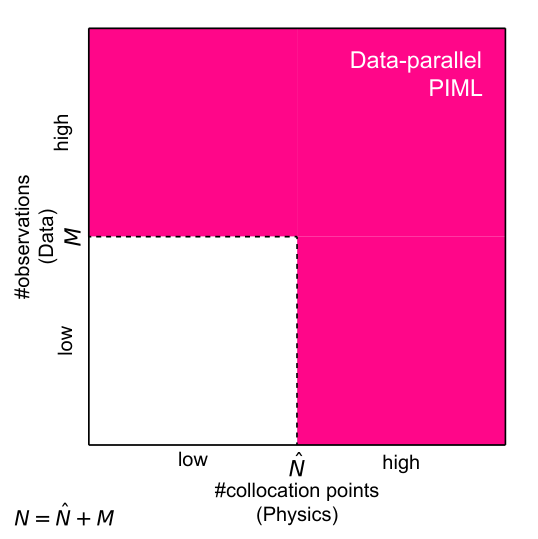
Any practitioner strives to reach the permanent regime for their PIML scheme, and we provide the necessary details for an easy implementation of Horovod-based data acceleration for PINNs, with direct application to any PIML model. Fig. 2 (left) further illustrates the scope of data-parallel PIML. For the sake of clarity, Fig. 2 (right) supplies a comprehensive review of important notations defined throughout this manuscript, along with their corresponding introductions.
| Notation | Definition | Eq. |
|---|---|---|
| Eq. (2) | ||
| Residual for | Eq. (3) | |
| # collocation points | Eq. (6) | |
| # observations | Eq. (6) | |
| # training points | Eq. (6) | |
| Training error | Eq. (18) | |
| Testing error | Eq. (18) | |
| Generalization error | Eq. (20) |
Next, we apply the procedure to increasingly complex problems and demonstrate that Horovod acceleration is straightforward, using the pioneer PINNs code of Raissi as an example. Our main practical findings concerning data-parallel PINNs for up to GPUs are the following :
- •
They do not require to modify their hyper-parameters;
- •
They show similar training convergence to the GPU-case;
- •
They lead to high efficiency for both weak and strong scaling (e.g for Navier-Stokes problem with 8 GPUs).
This work is organized as follows: In “Problem formulation”, we introduce the PDEs under consideration, PINNs and convergence estimates for the generalization error. We then move to “Data-parallel PINNs” and present “Numerical experiments”. Finally, we close this manuscript in “Conclusion”.
Problem formulation
General notation
Throughout, vector and matrices are expressed using bold symbols. For a natural number , we set . For , and an open set with , let be the standard class of functions with bounded -norm over . Given , we refer to[1, Section 2] for the definitions of Sobolev function spaces . Norms are denoted by , with subscripts indicating the associated functional spaces. For a finite set , we introduce notation , closed subspaces are denoted by a -symbol and .
Abstract PDE
In this work, we consider a domain , , with boundary . For any , , we solve a general non-linear PDE of the form:
| (1) |
with a spatio-temporal differential operator, the boundary conditions (BCs) operator, the material parameters—the latter being unknown for inverse problems—and for any . Accordingly, for any function defined over , we introduce
| (2) |
and define the residuals for each and any observation function :
| (3) |
PINNs
Following[20, 35], let be a smooth activation function. Given an input , we define as being a -layer neural feed-forward neural network with , and neurons in the -th layer for . For constant width DNNs, we set . For , let us denote the weight matrix and bias vector in the -th layer by and , respectively, resulting in:
| (4) |
This results in representation , with
| (5) |
the (trainable) parameters—or weights—in the network. We set . Application of PINNs to Eq. (1) yields the approximate .
We introduce the training dataset , , for and observations , . Furthermore, to each training point we associate a quadrature weight . All throughout this manuscript, we set:
| (6) |
Note that (resp. ) represents the amount of information for the data-driven (resp. physics) part, by virtue of the PIML paradigm (refer to Fig. 2). The network weights in Eq. (5) are trained (e.g., via ADAM optimizer[34]) by minimizing the weighted loss:
| (7) |
We seek at obtaining:
| (8) |
The formulation for PINNs addresses the cases with no data (i.e. ) or physics (i.e. ), thus exemplifying the PIML paradigm. Furthermore, it is able to handle time-independent operators with only minor changes; a schematic representation of a forward time-independent PINN is shown in Fig. 3.

Our setting assumes that the material parameters are known. If , one can solve the inverse problem by seeking:
| (9) |
Similarly, unique continuation problems[23], which assume incomplete information for and , are solved throughout PINNs without changes. Indeed, “2D Navier-Stokes” combines unique continuation problem and unknown parameters .
Automatic Differentiation
We aim at giving further details about back-propagation algorithms and their dual role in the context of PINNs:
- 1.
Training the DNN by calculating ;
- 2.
Evaluating the partial derivatives in and so as to compute the loss .
They consist in a forward pass to evaluate the output (and ), and a backward pass to assess the derivatives. To further elucidate back-propagation, we reproduce the informative diagram from[11] in Fig. 4.

TensorFlow includes reverse mode AD by default. Its cost is bounded with for scalar output NNs (i.e. for ). The application of back-propagation (and reverse mode AD in particular) to any training point is independent of other information, such as neighboring points or the volume of training data. This allows for data-parallel PINNs. Before detailing its implementation, we justify the -analysis through an abstract theoretical background.
Convergence estimates
To understand better how PINNs scale with , we follow the method in [22, 23] under a simple setting, allowing to control the data and physics counterparts in PIML. Set and define spaces:
| (10) |
We assume that Eq. (1) can be recast as:
| (11) | ||||
| (12) |
We suppose that Eq. (11) is well-posed and that for any , there holds that:
| (13) |
Eq. (11) is a stability estimate, allowing to control the total error by means of a bound on PINNs residual. Residuals in Eq. (3) are:
| (14) |
From the expression of residuals, we are interested in approximating integrals:
| (15) |
We assume that we are provided quadratures:
| (16) |
for weights and quadrature points such that for :
| (17) |
For any , the loss is defined as follows:
| (18) |
with and the training error for collocation points and observations respectively.
Notice that application of Eq. (17) to and yields:
| (19) |
We seek to quantify the generalization error:
| (20) |
We detail a new result concerning the generalization error for PINNs.
Theorem 1 (Generalization error for generic PINNs)
Under the presented setting, there holds that:
| (21) |
with .
Proof 1
Consider the setting of Theorem 1. There holds that:
The novelty of Theorem 1 is that it describes the generalization error for a simple case involving collocation points and observations. It states that the PINN generalizes well as long as the training error is low and that sufficient training points are used. To make the result more intuitive, we rewrite Eq. (21), with expressing the terms up to positive constants:
| (22) |
The generalization error depends on the training errors (which are tractable during training), parameters and and bias .
To return to -analysis, we now have a theoretical proof of the three regimes presented in “Introduction”. Let us assume that . For small values of or , the bound in Theorem 1 is too high to yield a meaningful estimate. Subsequently, the convergence is as , marking the transition regime. It is paramount for practitioners to reach the permanent regime when training PINNs, giving ground to data-parallel PINNs.
In general applications, the exact solution is not available. Moreover, it is relevant to determine whether is large enough. To this extent, we introduce a same cardinality testing (or validation) set. Interestingly, the entire analysis above and Theorem 1 remain valid for another set of testing points, with the testing error and set as in Eq. (18). The train-test gap, which is tractable, can be quantified as follows.
Theorem 2 (Train-test gap bound)
Under the presented setting, there holds that:
Proof 2
Consider the setting of Theorem 2. For and there holds that:
The bound in Theorem 1 is valuable as it allows to assess the quadrature error convergence—and the regime—with respect to the number of training points.
Data-parallel PINNs
Data-distribution and Horovod
In this section, we present the data-parallel distribution for PINNs. Let us set and define ranks (or workers):
each rank corresponding generally to a GPU. Data-parallel distribution requires the appropriate partitioning of the training points across ranks.
We introduce collocation points and observations, respectively, for each rank (e.g., a GPU) yielding:
with
| (23) |
Data-parallel approach is as follows: We send the same synchronized copy of the DNN defined in Eq. (4) to each rank. Each rank evaluates the loss and the gradient . The gradients are then averaged using an all-reduce operation, such as the ring all-reduce implemented in Horovod[26, 36], which is known to be bandwith optimal with respect to the number of ranks[36]. The process is illustrated in Figure 5 for . The ring-allreduce algorithm involves each of the size nodes communicating with two of its peers times [26].

It is noteworthy to observe that data generation for data-free PINNs (i.e. with ) requires no modification to existing codes, provided that each rank has a different seed for random or pseudo-random sampling. Horovod allows to apply data-parallel acceleration with minimal changes to existing code. Moreover, our approach and Horovod can easily be extended to multiple computing nodes. As pointed out in “Introduction”, Horovod supports popular DL backends such as TensorFlow, PyTorch and Keras. In Listing 1, we demonstrate how to integrate data-parallel distribution using Horovod with a generic PINNs implementation in TensorFlow 1.x. The highlighted changes in pink show the steps for incorporating Horovod, which include: (i) initializing Horovod; (ii) pinning available GPUs to specific workers; (iii) wrapping the Horovod distributed optimizer and (iv) broadcasting initial variables to the master rank being .
Weak and strong scaling
Two key concepts in data distribution paradigms are weak and strong scaling, which can be explained as follows: Weak scaling involves increasing the problem size proportionally with the number of processors, while strong scaling involves keeping the problem size fixed and increasing the number of processors. To reformulate:
- •
Weak scaling: Each worker has training points, and we increase the number of workers size;
- •
Strong scaling: We set a fixed total number of training points, and we split the data over increasing size workers.
We portray weak and strong scaling in Fig. 6 for a data-free PINN with . Each box represents a GPU, with the number of collocation points as a color. On the left of each scaling option, we present the unaccelerated case. Finally, we introduce the training time for size workers. This allows to define the efficiency and speed-up as:
Numerical experiments
Throughout, we apply our proceeding to three cases of interest:
- •
“1D Laplace” equation (forward problem);
- •
“1D Schrödinger” equation (forward problem);
- •
“2D Navier-Stokes” equation (inverse problem).
For each case, we perform a -analysis followed by Horovod data-parallel acceleration, which is applied to the domain training points (and observations for the Navier-Stokes case). Boundary loss terms are negligible due to the sufficient number of boundary data points.
Methodology
We perform simulations in single float precision on a AMAX DL-E48A AMD Rome EPYC server with 8 Quadro RTX 8000 Nvidia GPUs—each one with a 48 GB memory. We use a Docker image of Horovod 0.26.1 with CUDA 12.1, Python 3.6.9 and Tensorflow 2.6.2. All throughout, we use tensorflow.compat.v1 as a backend without eager execution.
All the results are ready for use in HorovodPINNs GitHub repository and fully reproducible, ensuring also compliance with FAIR principles (Findability, Accessibility, Interoperability, and Reusability) for scientific data management and stewardship [37]. We run experiments times with seeds defined as:
in order to obtain rank-varying training points. For domain points, Latin Hypercube Sampling is performed with pyDOE 0.3.8. Boundary points are defined over uniform grids.
We use Glorot uniform initialization [3, Chapter 8]. “Error” refers to the -relative error taken over , and “Time” stands for the training time in seconds. For each case, the loss in Eq. (7) is with unit weights and Monte-Carlo quadrature rule for . Also, we set the volume of domain and
We introduce the time to perform iterations. The training points processed by second is as follows:
| (24) |
For the sake of simplicity, we summarize the parameters and hyper-parameters for each case in Table 1.
| Case | learning rate | width | depth | iterations | |||
| 1D Laplace | |||||||
| 1D Schrödinger | |||||||
| 2D Navier-Stokes |
1D Laplace
We first consider the 1D Laplace equation in as being:
| (25) |
Acknowledge that . We solve the problem for:
We set and . Points in are generated randomly over , and . The residual in Eq. (3):
yields the loss:
-analysis
We perform the -analysis for the error as portrayed before in Figure 1. The asymptotic regime occurs between and , with a precision of in accordance with general results for -analysis of traditional solvers. The permanent regime shows a slight improvement in accuracy, with mean “Error” dropping from for to for . To complete the -analysis, Figure 7 shows the convergence results of ADAM optimizer for all the values of . This plot reveals that each regime exhibits similar patterns. The high variability in convergence during the transition regime is particularly interesting, with some runs converging and others not. In the permanent regime, the convergence shows almost identical and stable patterns irrespective of .
Furthermore, we plot the training and test losses in Figure 8. Acknowledge that the validation loss and “Error” show similar behaviors. We use this figure as a reference to define each transition regime. In particular, it hints that the permanent regime is reached for as the relative error at best iteration between and drops from to . For the sake of precision, the value for is .
Data-parallel implementation
We set and compare both weak and strong scaling to original implementation, referred to as “no scaling”.
We provide a detailed description of Fig. 9, as it will serve as the basis for future cases:
- •
Left-hand side: Error for corresponding to .
- •
Middle: Error for weak scaling with and for ;
- •
Right-hand side: Error for strong scaling with and for
To reduce ambiguity, we use the -superscript for no scaling, as is performed over rank. The color for each violin box in the figure corresponds to the number of domain collocation points used for each GPU.
Fig. 9 demonstrates that both weak and strong scaling yield similar convergence results to their unaccelerated counterpart. This result is one of the main findings in this work: PINNs scale properly with respect to accuracy, validating the intuition behind -analysis and justifying the data-parallel approach. This allows one to move from pre-asymptotic to permanent regime by using weak scaling, or leverage the cost of a permanent regime application by dispatching the training points over different workers. Furthermore, the hyper-parameters, including the learning rate, remained unchanged.
Next, we summarize the data-parallelization results in Table 2 with respect to size.
| size | Weak scaling | Strong scaling | Weak scaling | Strong scaling |
In the first column, we present the time required to run iterations for ADAM, referred to as . This value is averaged over one run of iterations with a heat-up of iteration (i.e. we discard the values corresponding to iterations and ). We present the resulting mean value standard deviation for the resulting vector. The second column, displays the efficiency of the run, evaluated with respect to .
Table 2 reveals that data-based acceleration results in supplementary training times as anticipated. Weak scaling efficiency varies between for to for , resulting in a speed-up of when using GPUs. Similarly, strong scaling shows similar behavior. Furthermore, it can be observed that yields almost equal for () and ().
To conclude, the Laplace case is not reaching its full potential with Horovod due to the small batch size . However, increasing the value of in next cases will lead to a noticeable increase in efficiency.
1D Schrödinger
We solve the non-linear Schrödinger equation along with periodic BCs (refer to [10, Section 3.1.1]) given over with and :
where . We apply PINNs to the system with in Eq. (4) as . We set .
-analysis
To begin with, we perform the -analysis for the parameters in Fig. 10.
Again, the transition regime for the total execution time distribution begins at a density of and spans between and . At higher magnitudes of , the error remains approximately the same. To illustrate this more complex case, we present the total execution time distribution in Fig. 11.
We note that the training times remain stable for . This observation is of great importance and should be emphasized, as it adds additional parameters to the analysis. Our work primarily focuses on error in -analysis, however, execution time and memory requirements are also important considerations. We see that in this case, weak scaling is not necessary (the optimal option is to use and ). Alternatively, strong scaling can be done with .
To gain further insight into the variability of the transition regime, we focus on . We compare the solution for and in Fig. 12.


The upper figures depict predicted by the PINN. The lower figures show a comparison between the exact and predicted solutions are plotted for . It is evident that the solution for closely resembles the exact solution, whereas the solution for fails to accurately represent the solution near , thereby illustrating the importance of achieving a permanent regime. Next, we show the training and testing losses in Fig. 13. We remark that the training and test losses converge for . Analysis of the train-test gap showed that it converged as . Visually, one can assume that the losses are close enough for (or ), in accordance with the -analysis performed in Fig. 10.
Data-parallel implementation
We compare the error for unaccelerated and data-parallel implementations of simulations for in Fig. 14, analogous to the analysis in Fig. 9.
Again, the error is stable with size. Both no scaling and weak scaling are similar. Strong scaling is unaffected by size. We plot the training time in Fig. 15.
We observe that both weak and strong scaling increase linearly and slightly with size. Both scaling show similar behaviors. Fig. 16 portrays the number of training points processed per second (refer to Eq. (24)) and the efficiency with respect to size, with white bars representing the ideal scaling. Efficiency shows a gradual decrease with size, with results surpassing those of the previous section. The efficiency for reaches and respectively for weak and strong scaling, representing a speed-up of and .
Inverse problem: Navier-Stokes equation
We consider the Navier-Stokes problem with , and unknown parameters . The resulting divergence-free Navier Stokes is expressed as follows:
| (26) |
wherein and are the and components of the velocity field, and the pressure. We assume that there exists such that:
| (27) |
Under Eq. (27), last row in Eq. (26) is satisfied. The latter leads to the definition of residuals:
We introduce pseudo-random points and observations , yielding the loss:
with
Throughout this case, we have , and we plot the results with respect to . Acknowledge that , and that both and the BCs are unkwown.
-analysis
We conduct the -analysis and show the error in Fig. 17, showing no differences with previous cases.
Surprisingly, the permanent regime is reached only for , despite the problem being a -dimensional, non-linear, and inverse one. This corresponds to low values of , indicating that PINNs seem to prevent the curse of dimensionality. In fact, the it was achieved with only points per unit per dimension. The total training time is presented in Fig. 18, where it can be seen to remain stable up to , and then increases linearly with .
Again, we represent the training and test losses in Fig. 19. The train-test gap is shown to decrease for as . Furthermore, the train-test gap can be considered as being small enough, visually, for .
Data-parallel implementation
We run the data-parallel simulations, setting . As shown in Fig. 20, the simulations exhibit stable accuracy with size.
The execution time increases moderately with size, as illustrated in Fig. 21. The training time decreases with for the no scaling case. However, this behavior is temporary (refer to Fig. 17 before).
We conclude our analysis by plotting the efficiency with respect to size in Fig. 22. Efficiency lowers with increasing size, but shows the best results so far, with (resp. ) weak (resp. strong) scaling efficiency for . For the sake of completeness, the weak efficiency for and improved to . This encouraging result sets the stage for further exploration of more intricate applications.
Conclusion
In this work, we proposed a novel data-parallelization approach for PIML with a focus on PINNs. We provided a thorough -analysis and associated theoretical results to support our approach, as well as implementation considerations to facilitate implementation with Horovod data acceleration. Additionally, we ran reproducible numerical experiments to demonstrate the scalability of our approach. Further work include the implementation of Horovod acceleration to DeepXDE[35] library, coupling of localized PINNs with domain decomposition methods, and application on larger GPU servers (e.g., with more than 100 GPUs).
Data availability
The code required to reproduce these findings are available to download from https://github.com/pescap/HorovodPINNs.
References
- [1] Steinbach, O. Numerical Approximation Methods for Elliptic Boundary Value Problems: Finite and Boundary Elements. Texts in Applied Mathematics (Springer New York, 2007).
- [2] LeCun, Y., Bengio, Y. & Hinton, G. Deep learning. \JournalTitlenature 521, 436–444 (2015).
- [3] Bengio, Y., Goodfellow, I. & Courville, A. Deep learning, vol. 1 (MIT press Cambridge, MA, USA, 2017).
- [4] Karniadakis, G. E. et al. Physics-informed machine learning. \JournalTitleNature Reviews Physics 3, 422–440, DOI: https://doi.org/10.1038/s42254-021-00314-5 (2021).
- [5] You, H., Yu, Y., Trask, N., Gulian, M. & D’Elia, M. Data-driven learning of nonlocal physics from high-fidelity synthetic data. \JournalTitleComputer Methods in Applied Mechanics and Engineering 374, 113553, DOI: https://doi.org/10.1016/j.cma.2020.113553 (2021).
- [6] Sun, L., Gao, H., Pan, S. & Wang, J.-X. Surrogate modeling for fluid flows based on physics-constrained deep learning without simulation data. \JournalTitleComputer Methods in Applied Mechanics and Engineering 361, 112732, DOI: https://doi.org/10.1016/j.cma.2019.112732 (2020).
- [7] Lai, Z. et al. Neural Modal ODEs: Integrating Physics-based Modeling with Neural ODEs for Modeling High Dimensional Monitored Structures. \JournalTitlearXiv preprint arXiv:2207.07883 (2022).
- [8] Lai, Z., Mylonas, C., Nagarajaiah, S. & Chatzi, E. Structural identification with physics-informed neural ordinary differential equations. \JournalTitleJournal of Sound and Vibration 508, 116196, DOI: https://doi.org/10.1016/j.jsv.2021.116196 (2021).
- [9] Alber, M. et al. Integrating machine learning and multiscale modeling—perspectives, challenges, and opportunities in the biological, biomedical, and behavioral sciences. \JournalTitleNPJ digital medicine 2, 1–11, DOI: https://doi.org/10.1038/s41746-019-0193-y (2019).
- [10] Raissi, M., Perdikaris, P. & Karniadakis, G. Physics-informed neural networks: A deep learning framework for solving forward and inverse problems involving nonlinear partial differential equations. \JournalTitleJournal of Computational Physics 378, 686–707, DOI: https://doi.org/10.1016/j.jcp.2018.10.045 (2019).
- [11] Baydin, A. G., Pearlmutter, B. A., Radul, A. A. & Siskind, J. M. Automatic Differentiation in Machine Learning: A Survey. \JournalTitleJ. Mach. Learn. Res. 18, 5595–5637, DOI: https://doi.org/10.5555/3122009.3242010 (2017).
- [12] Chen, Y., Lu, L., Karniadakis, G. E. & Negro, L. D. Physics-informed neural networks for inverse problems in nano-optics and metamaterials. \JournalTitleOpt. Express 28, 11618–11633, DOI: https://doi.org/10.1364/OE.384875 (2020).
- [13] Chen, X., Duan, J. & Karniadakis, G. E. Learning and meta-learning of stochastic advection–diffusion–reaction systems from sparse measurements. \JournalTitleEuropean Journal of Applied Mathematics 32, 397–420, DOI: https://doi.org/10.1017/S0956792520000169 (2021).
- [14] Meng, X. & Karniadakis, G. E. A composite neural network that learns from multi-fidelity data: Application to function approximation and inverse PDE problems. \JournalTitleJournal of Computational Physics 401, 109020, DOI: https://doi.org/10.1016/j.jcp.2019.109020 (2020).
- [15] Li, R., Wang, J.-X., Lee, E. & Luo, T. Physics-informed deep learning for solving phonon Boltzmann transport equation with large temperature non-equilibrium. \JournalTitlenpj Computational Materials 8, 1–10, DOI: https://doi.org/10.1038/s41524-022-00712-y (2022).
- [16] Yang, X. I. A., Zafar, S., Wang, J.-X. & Xiao, H. Predictive large-eddy-simulation wall modeling via physics-informed neural networks. \JournalTitlePhys. Rev. Fluids 4, 034602, DOI: https://doi.org/10.1103/PhysRevFluids.4.034602 (2019).
- [17] Zhang, D., Lu, L., Guo, L. & Karniadakis, G. E. Quantifying total uncertainty in physics-informed neural networks for solving forward and inverse stochastic problems. \JournalTitleJournal of Computational Physics 397, 108850, DOI: https://doi.org/10.1016/j.jcp.2019.07.048 (2019).
- [18] Escapil-Inchauspé, P. & Ruz, G. A. Physics-informed neural networks for operator equations with stochastic data, DOI: https://doi.org/10.48550/ARXIV.2211.10344 (2022).
- [19] Wang, S., Yu, X. & Perdikaris, P. When and why PINNs fail to train: A neural tangent kernel perspective. \JournalTitleJournal of Computational Physics 449, 110768, DOI: https://doi.org/10.1016/j.jcp.2021.110768 (2022).
- [20] Escapil-Inchauspé, P. & Ruz, G. A. Hyper-parameter tuning of physics-informed neural networks: Application to Helmholtz problems. \JournalTitlearXiv preprint arXiv:2205.06704 (2022).
- [21] Shukla, K., Xu, M., Trask, N. & Karniadakis, G. E. Scalable algorithms for physics-informed neural and graph networks. \JournalTitleData-Centric Engineering 3, e24, DOI: https://doi.org/10.1017/dce.2022.24 (2022).
- [22] Mishra, S. & Molinaro, R. Estimates on the generalization error of physics-informed neural networks for approximating PDEs. \JournalTitleIMA Journal of Numerical Analysis DOI: https://doi.org/10.1093/imanum/drab093 (2022).
- [23] Mishra, S. & Molinaro, R. Estimates on the generalization error of physics-informed neural networks for approximating a class of inverse problems for PDEs. \JournalTitleIMA Journal of Numerical Analysis 42, 981–1022, DOI: https://doi.org/10.1093/imanum/drab032 (2021).
- [24] Shin, Y., Darbon, J. & Karniadakis, G. E. On the convergence of physics informed neural networks for linear second-order elliptic and parabolic type PDEs. \JournalTitlearXiv preprint arXiv:2004.01806 (2020).
- [25] Khoo, Y., Lu, J. & Ying, L. Solving parametric PDE problems with artificial neural networks. \JournalTitleEuropean Journal of Applied Mathematics 32, 421–435 (2021).
- [26] Sergeev, A. & Del Balso, M. Horovod: fast and easy distributed deep learning in TensorFlow. \JournalTitlearXiv preprint arXiv:1802.05799 (2018).
- [27] Jagtap, A. D., Kharazmi, E. & Karniadakis, G. E. Conservative physics-informed neural networks on discrete domains for conservation laws: Applications to forward and inverse problems. \JournalTitleComputer Methods in Applied Mechanics and Engineering 365, 113028, DOI: https://doi.org/10.1016/j.cma.2020.113028 (2020).
- [28] Jagtap, A. D. & Karniadakis, G. E. Extended Physics-Informed Neural Networks (XPINNs): A Generalized Space-Time Domain Decomposition Based Deep Learning Framework for Nonlinear Partial Differential Equations. \JournalTitleCommunications in Computational Physics 28, 2002–2041, DOI: https://doi.org/10.4208/cicp.OA-2020-0164 (2020).
- [29] Hu, Z., Jagtap, A. D., Karniadakis, G. E. & Kawaguchi, K. When Do Extended Physics-Informed Neural Networks (XPINNs) Improve Generalization? \JournalTitleSIAM Journal on Scientific Computing 44, A3158–A3182, DOI: https://doi.org/10.1137/21M1447039 (2022).
- [30] Dwivedi, V., Parashar, N. & Srinivasan, B. Distributed physics informed neural network for data-efficient solution to partial differential equations. \JournalTitlearXiv preprint arXiv:1907.08967 (2019).
- [31] Shukla, K., Jagtap, A. D. & Karniadakis, G. E. Parallel physics-informed neural networks via domain decomposition. \JournalTitleJournal of Computational Physics 447, 110683, DOI: https://doi.org/10.1016/j.jcp.2021.110683 (2021).
- [32] McClenny, L. D., Haile, M. A. & Braga-Neto, U. M. TensorDiffEq: Scalable Multi-GPU Forward and Inverse Solvers for Physics Informed Neural Networks. \JournalTitlearXiv preprint arXiv:2103.16034 (2021).
- [33] Hennigh, O. et al. NVIDIA SimNet™: An AI-accelerated multi-physics simulation framework. In Computational Science–ICCS 2021: 21st International Conference, Krakow, Poland, June 16–18, 2021, Proceedings, Part V, 447–461 (Springer, 2021).
- [34] Kingma, D. P. & Ba, J. Adam: A method for stochastic optimization. \JournalTitlearXiv preprint arXiv:1412.6980 (2014).
- [35] Lu, L., Meng, X., Mao, Z. & Karniadakis, G. E. DeepXDE: A Deep Learning Library for Solving Differential Equations. \JournalTitleSIAM Review 63, 208–228, DOI: https://doi.org/10.1137/19M1274067 (2021). https://doi.org/10.1137/19M1274067.
- [36] Patarasuk, P. & Yuan, X. Bandwidth optimal all-reduce algorithms for clusters of workstations. \JournalTitleJournal of Parallel and Distributed Computing 69, 117–124 (2009).
- [37] Wilkinson, M. D. et al. The fair guiding principles for scientific data management and stewardship. \JournalTitleScientific data 3, 1–9 (2016).
Acknowledgements
The authors would like to thank the Data Observatory Foundation, ANID FONDECYT 3230088, FES-UAI postdoc grant, ANID PIA/BASAL FB0002, and ANID/PIA/ANILLOS ACT210096, for financially supporting this research.
Author contributions statement
P.E.I. conceived the experiment(s). All authors analyzed the results and reviewed the manuscript.