Graphical estimation of multivariate count time series
Abstract
The problems of selecting partial correlation and causality graphs for count data are considered. A parameter driven generalized linear model is used to describe the observed multivariate time series of counts. Partial correlation and causality graphs corresponding to this model explain the dependencies between each time series of the multivariate count data. In order to estimate these graphs with tunable sparsity, an appropriate likelihood function maximization is regularized with an -type constraint. A novel MCEM algorithm is proposed to iteratively solve this regularized MLE. Asymptotic convergence results are proved for the sequence generated by the proposed MCEM algorithm with -type regularization. The algorithm is first successfully tested on simulated data. Thereafter, it is applied to observed weekly dengue disease counts from each ward of Greater Mumbai city. The interdependence of various wards in the proliferation of the disease is characterized by the edges of the inferred partial correlation graph. On the other hand, the relative roles of various wards as sources and sinks of dengue spread is quantified by the number and weights of the directed edges originating from and incident upon each ward. From these estimated graphs, it is observed that some special wards act as epicentres of dengue spread even though their disease counts are relatively low.
keywords
graphical models, count data, partial correlation, Monte Carlo expectation and maximization, -type regularization.1 Introduction
The dependencies between multiple interdependent time series data, such as the temperatures recorded from neighbouring geographical regions (Bach and Jordan 2004), stock prices from related markets (David A. Bessler 2003), biological signals that measure activities in the human brain (Qian et al. 2015) etc, are studied using graphical models. In a graphical model, each data series is represented as a vertex of a graph and the dependencies between the different time series are represented by edges in the graph. In many applications such as finance, insurance, biomedical, public health, etc, time series data is frequently measured in the form of counts (Mehdi Jalalpour and Levin 2015; R.K.Freeland and McCabe 2004). In this paper, we propose a novel algorithm for inferring the dependencies and the strength of the dependencies (i.e., the graphical model) for multiple inter-related count time series data. The algorithm is applied to discover the spreading pattern of dengue infections in a large Indian city.
In graphical models, the dependencies between multiple time series are represented either by undirected or directed graphs (e.g., see W. J. Granger 1969; Eichler 2012; Dahlhaus and Eichler 2003; Jung et al. 2015 and references therein). First we review the undirected graphical models in brief and thereafter review the directed graphical models. Graphical models were introduced initially for multiple random variables in (Dempster 1972) using the inverse covariance matrix of the associated random vectors. (Brillinger 1996) introduced such models for multivariate time series, where the dependencies between the nodes were represented using partial correlations. In (Songsiri et al. 2009) and (Dahlhaus 2000), graphical description of vector autoregressive (AR) models were considered for stationary time series and defined in terms of the inverse spectral density matrix. These results were extended to graphical models with vector autoregressive moving average (ARMA) models in (Avventi et al. 2013). In (Songsiri and Vandenberghe 2010), a method to control the sparsity of the estimated graph was introduced through an -type regularization. Such a regularization (often called Least Absolute Shrinkage and Selection Operator (LASSO)) on the standard maximum likelihood estimation (MLE) method, reduces overfitting and provides control over the sparsity of the estimated graphical model (Tibshirani 1996).
Directed graphical models were introduced in (Wright 1921; Wright 1934) as path diagrams for the study of hereditary properties, linking parents and children graphically by arrows. For multivariate time series, one series is said to be causal for another series if the prediction of second series using all available information except the first series, can be improved by adding the available information about the first series. This definition of the so-called Granger causality was introduced in (W. J. Granger 1969). Using this notion, the causalities between multiple time series were represented as directed Granger causality graphs, where each time series was represented as a vertex and the causality between two different time series was represented by a directed edge (Sims 1972; Pierce and Haugh 1977). The multivariate autoregressive (AR) model of second order stationary time series was used to obtain Granger causality graph (TjØstheim 1981; Hsiao 1982) where the causalities between multiple time series were calculated directly from the autoregressive coefficients. The Granger causality graphs were studied by (Eichler 2006; Eichler 2007) through multivariate autoregressive (AR) models of second order stationary time series. Later, sparse Granger causality graphs were discussed in (Songsiri 2013; Songsiri 2015; Zorzi and Sepulchre 2016; Alpago et al. 2018; Ciccone et al. 2018) through multivariate AR time series.
In all the above papers, the graphical models were discussed for time series of Gaussian data. In contrast to the graphical models for Gaussian data, literature on graphical models for count data is still sparse. The undirected graphical models were introduced for multivariate count data in (Park and Park 2019) using a Bayesian approach to inference. Later, the undirected graphical models were considered for multivariate count data in (Roy and Dunson 2020) to obtain the complex interactions between genes using a pseudo-likelihood based algorithm. Unlike these directed models, Poisson directed acyclic graphical (DAG) models, also referred to as Bayesian Networks (Park and Raskutti 2015; Park and Raskutti 2017), were obtained for multivariate count data in (Hue and Chiogna 2021). In all these papers, the graphical models are obtained for multiple random variables. In contrast, our aim in this paper is to estimate undirected and directed graphical model for multivariate count time series where the dependencies between these time series are represented using causalities and partial correlations.
To model count time series, generalized linear models (GLM) were discussed in (Zeger and Qaqish 1988; Li 1994; Fahrmeir and Tutz 2001; Fahrmeir and Wagenpfeil 1997; Durbin and Koopman. 2000). In (Utazi et al. 2018), parameter driven models were used for modeling multivariate time series of counts, using a latent process to account for the correlation between the observed counts. In this paper, we choose this model for our study. In this model, the latent process is unknown. While the unknown parameters in such models can, in principle, be estimated using the well known expectation and maximization (EM) algorithm (Dempster et al. 1977), associated difficulties in calculating the conditional density functions requires us to use the the Monte Carlo expectation and maximization (MCEM) algorithm (Wei and Tanner 1990; Chan and Ledolter 1995). In this paper, we extend a combination of the methods from (Dempster et al. 1977; Wei and Tanner 1990; Chan and Ledolter 1995) to infer graphical models with tunable sparsity, using LASSO.
First we introduce certain choices about the model, formulation and methodology. Following (W. J. Granger 1969; Songsiri and Vandenberghe 2010), the dependencies between the observed multivariate time series of counts are represented using partial correlations and causalities. However partial correlations and causalities between multiple time series can only be calculated easily for second order stationary time series. In our case, the observed count data is usually non stationary, e.g., the data might be seasonal in nature or follow various trends (Fahrmeir and Tutz 1994). To address this issue, we introduce an unobserved multivariate second order stationary latent process to calculate the partial correlation and causality between the observed multiple count time series. We define the partial correlation and causality between elements of the observed time series in terms of the partial correlation and causality between elements of the stationary latent processes. As in (Chan and Ledolter 1995), the observed count data given the latent process, follows a Poisson distribution, while the multivariate latent process follows an autoregressive (AR) Gaussian model.
It is known that the partial correlation between multiple time series can be computed from the inverse spectral density matrix of a multivariate stationary time series (Brillinger 1981). Thus the partial correlations for the stationary latent process in our model are obtained in terms of the parameters of the latent AR model (Brockwell and Davis 2002) using the inverse spectral density matrix. Further, to obtain the partial correlations and causalities for the observed multivariable count data from the stationary latent process, we need to estimate unknown parameters of the AR model. Since the number of possible edges in the partial correlation graph can be large, overfitting can be a potential issue in this estimation problem (Cawley and Talbot 2010). Thus a maximum likelihood estimation (MLE), with -type regularization term involving the partial correlation constraints, is formulated to get the desired sparsity in the estimated partial correlation and causality graph. Since the latent process is unknown, a direct maximization of the log-likelihood function with -type regularization is not possible. Following (Chan and Ledolter 1995), an MCEM algorithm with -type regularization is proposed to estimate the model parameters. In this algorithm, samples from the conditional density function of the latent process given observed data, are generated using the Metropolis-Hastings algorithm (Chan and Ledolter 1995).
First, the proposed MCEM algorithm with -type regularization is tested on a simulated multivariable count dataset. The regularization parameter is estimated using the trade-off curve (Songsiri 2010) between log-likelihood and -type regularization function. We collect all the graphs along the trade-off curve for different values of regularization parameter and then choose the partial correlation and causality graph based on the Bayes information criterion (BIC)(Songsiri 2010).
Next, we use the developed algorithm to estimate the partial correlation and causality graphs for the observed dengue disease data. The dengue data under investigation consist of weekly dengue counts in a six year period, January to December , collected from each ward of Greater Mumbai city, India. From these estimated partial correlation and causality graphs, we infer the number of undirected, incoming and outgoing edges for each ward. These edges and their weights give a quantitative measure of the interdependence and directionality of the disease prevalence and development in the various wards. Surprisingly, we observe that some wards act as the epicentres of disease spread even though their absolute disease counts are relatively low.
This manuscript is an extended version of (Sathish et al. 2019) which was presented in IEEE 58th Conference on Decision and Control (CDC), December 2019. It differs from (Sathish et al. 2019) as follows:
- 1.
In this manuscript, in addition to the problem of estimating partial correlation graphs studied in (Sathish et al. 2019), the problem of estimating causality graphs is also considered. Causality graphs were not studied in (Sathish et al. 2019).
- 2.
No real world application was presented in (Sathish et al. 2019). Here, the developed algorithms are applied on observed weekly dengue disease counts in each of the 24 wards of Greater Mumbai city from 2010- 2015, to learn directed and undirected models for the spread of dengue disease.
Our contributions in this paper are as follows.
- 1.
We formulate an optimization problem of maximum likelihood estimation (MLE) of observed multivariate count data with -type regularization to estimate the partial correlation and causality graphs.
- 2.
A Monte Carlo expectation and maximization (MCEM) algorithm with -type regularization on multivariate count data is proposed to solve the formulated problem.
- 3.
The proposed MCEM algorithm with -type regularization is tested successfully using simulated data.
- 4.
The partial correlation and causality graphs are estimated for the observed weekly dengue disease counts from each ward of Greater Mumbai city.
2 Preliminaries and problem formulation
2.1 Parameter driven model
Let { be an observed multivariate time series of counts. An unobserved multivariate second order stationary latent process { is used to introduce the correlation between observations measured at successive time points and individual time series. To model using , a parameter driven model introduced in (Utazi et al. 2018) is considered. Let be a vector of covariates at time for the th time series and be a vector of regression coefficients corresponding to the th covariate vector . Covariate vector is a function of time and is usually used to model the explanatory variables such as trend, seasonality etc. In this model, the counts , given the latent process and the covariates , follow Poisson distribution with conditional mean , which is denoted by
| (1) |
We assume the latent process in the model (1) follows an AR(p) process given by
| (2) |
where ’s are autoregressive coefficients and is a Gaussian white noise having zero mean and variance . Let = {} be an matrix of autoregressive coefficients and := () be iid Gaussian random variables with covariance matrix := diag(). For , the vector notation of the AR(p) multivariate latent process is given by
| (3) |
Let and . Also assume that the parameter space is denoted by . Define the operator vec(), which converts the matrix into a vector by setting columns of the matrix as a vector. Then, represents the complete set of unknown parameters described by models (1) and (3).
2.2 Partial correlation graphs
Let be a mixed graph (graph with directed and undirected edges), where is a set of vertices, is a set of undirected edges and is a set of directed edges . The undirected edge between vertices and is denoted as . If then also . The directed edge between vertices and with direction from to is denoted as . If then .
Let denote except the th and th elements i.e., and and denote except and . The partial correlation between any two time series of multivariate second order stationary processes is given in (Dahlhaus 2000). Define
| (4) |
as the error process between and best linear filter based on that minimizes . Here and are the optimal linear filters, exact expressions for which are available in (Brillinger 1981). Similarly, the error process for is . If the cross-covariance between and for all time lag is zero, i.e., , , then and are defined to be partially uncorrelated given .
From (W. J. Granger 1969), the process is said to be causal for the another process if the prediction of using all available information except , can be improved by adding the available information about .
We define the partial correlations and causalities between observed time series of counts in terms of the partial correlations and causalities between second order stationary latent processes as follows.
Definition 1.
Two time series and are partially uncorrelated given if and are partially uncorrelated given and is not causal for if is not causal for .
Now, the partial correlation and causality graph for the multivariate time series is defined as,
Definition 2 (Partial correlation and causality graph of ).
The Partial correlation and causality graph of modeled in (1) and (3) is the mixed graph with vertex set , undirected edge set and directed edge set such that there is no undirected edge between the and the node if and only if the corresponding latent variables and are partially uncorrelated given , and there is no directed edge from the to the node if and only if is not causal for .
Let be the autocovariance function of with time lag and be the spectral density matrix of i.e.,
| (5) |
It is known that the partial correlation graph can be obtained from the inverse spectral density matrix of multivariate second order stationary process (Brillinger 1981) which is given in the theorem below.
Theorem 3.
(Brillinger 1981) Consider the stationary time series and assume that the spectral density matrix of is invertible for all . Then, and are partially uncorrelated given if and only if .
Thus from (Songsiri and Vandenberghe 2010) and Theorem 3, the partial correlation relations for the stationary latent process , which follows an AR model (3), in terms of inverse spectral are given in the lemma below.
Lemma 4.
where
| (6) |
with .
Proposition 5.
and are partially uncorrelated given if .
The following theorem states that the causality graph of the second order stationary process can be found in terms of AR coefficients given in (3) (TjØstheim 1981; Hsiao 1982).
Theorem 6.
The time series does not cause if and only if the corresponding components vanish for all i.e.,
| (7) |
The following definitions are useful for future development in later sections. Let be the total incoming edge weight of node from other nodes in the causality graph, i.e.,
| (8) |
Similarly, let be the total outgoing edge weight of node to other nodes in the causality graph, i.e.,
| (9) |
2.3 Problem formulation
From Theorem 3 and Proposition 5, we need to estimate the inverse spectral density matrix of multivariate latent process to estimate the partial correlations between the observed multiple time series of counts . Since the number of possible edges in the partial correlation and causality graph can be large (up to ), overfitting can be a potential issue in this estimation problem (Cawley and Talbot 2010). LASSO (Tibshirani 1996) is one of the regularization methods to overcome this difficulty by setting certain parameters to zero. This technique is used here to introduce sparsity in the inverse spectral density matrix. In LASSO, the maximum likelihood estimation problem is regularized using the -norm of the partial correlation constraints given in Proposition 5. The -norm of a vector is defined as . Let be the observed data matrix and be the latent process data matrix. From (Utazi et al. 2018), the joint probability density function (PDF) of and is
| (10) |
where and is the joint probability density function of initial values . The calculation of probability density function is given in (Helmut 2005), p.29. Let
| (11) |
Then, the model (3) becomes
| (12) |
Note that is a second-order stationary process, and and are uncorrelated. Thus, from (12) the auto-covariance function of with zero time lag is
| (13) |
where
| (14) |
The vectorized equation of (13) is
| (15) |
where ‘’ denotes the Kronecker product. Therefore, the initial values follows a Gaussian distribution (Helmut 2005) with zero mean and variance is which can be calculated from (2.3).
The exact log-likelihood function of and is . Let
| (16) |
where is a regularization parameter and the regularization function is the -norm of off-diagonal elements of matrices given in (6). The amount of sparsity of the estimated inverse spectral density matrix is controlled by the regularization parameter . As varies, the sparsity pattern varies in the estimated inverse spectral density matrix from dense ( small) to diagonal ( large). We aim to maximize regularized log-likelihood with respect to over to estimate the optimal parameters. To maximize directly, data matrix should be known. However, in reality the latent data matrix is unknown. The marginal PDF of is . Let be the marginal log-likelihood of . The marginal log-likelihood of with -type regularization
| (17) |
is used to estimate . We next formulate the optimization problem to estimate .
Problem 2.1.
Find
| (18) |
2.4 Challenges in solution of Problem 2.1
To solve Problem 2.1 directly, we need to calculate explicitly, which can be difficult because of multiple integrals. To overcome this difficulty and unknown latent data matrix , we use the expectation and maximization (EM) algorithm (Dempster et al. 1977) to solve Problem 2.1. The EM algorithm maximizes the function by working with and the conditional density function of the latent data matrix given observed count data matrix .
Note that the standard EM algorithm is modified with the regularization term in the following Algorithm 2.1. The tolerance () is adjusted according to the accuracy requirement in the estimated parameters.
| (19) |
The log-likelihood function is required to be known to solve the Algorithm 2.1. However, the conditional density function of the latent data matrix given observed count data matrix is impossible to calculate at the th step in the Algorithm 2.1 because it is a mixture of Gaussian and Poisson distributions. Here Algorithm 2.1 cannot be implemented directly. To overcome this difficulty, Monte Carlo techniques are used to draw samples from and thereby numerically compute the integral given in the E-step of Algorithm 2.1. The Metropolis-Hastings algorithm (Casella and Berger 2002) is used to generate the samples from .
The generation of samples from using Metropolis-Hastings algorithm for the parameter driven model with AR(1) process is given in (Utazi et al. 2018). In (Utazi et al. 2018), the proposal distributions are calculated in Metropolis-Hastings algorithm with AR(1) process. Similarly, in this paper the proposal distributions for Metropolis-Hastings algorithm with AR(p) process are given. Let
| (20) |
For , the proposal distribution of given from the past, and to the future follows a Gaussian distribution with variance,
| (21) |
and mean,
| (22) |
For , the proposal distribution of given from the past, and to the future follows a Gaussian distribution with variance,
| (23) |
and mean,
| (24) |
For , the proposal distribution of given from the past, and to the future follows a Gaussian distribution with variance,
| (25) |
and mean,
| (26) |
Using these proposal distributions in Metropolis-Hastings algorithm given in Algorithm 2.2, we generate samples , ,…, from conditional density function . Thus, we propose a Monte Carlo expectation and maximization (MCEM) algorithm with -type regularization next.
3 Main results
In this section we discuss the Monte Carlo expectation and maximization (MCEM) algorithm with -type regularization. Further, the asymptotic convergence of sequence of parameters generated by the MCEM algorithm with -type regularization is proved.
3.1 Monte Carlo Expectation and Maximization (MCEM) algorithm with -type regularization
In this section, we propose a MCEM algorithm with -type regularization to estimate parameters . As mentioned above, we approximate the integral in the - (step 2) of Algorithm 2.1. The MCEM algorithm with -type regularization is presented in Algorithm 3.1. The tolerance () is adjusted according to the accuracy requirement in the estimated parameters.
From this algorithm, the generated sequence is {} and the estimated parameter is . This estimated parameter is the local maximizer of the function . We prove this claim in the next section. Note that the generated sequence {} is a sequence of random variables.
3.2 Asymptotic results
We obtain the sequence {} from the Monte Carlo expectation and maximization (MCEM) algorithm with -type regularization given in Algorithm 3.1. We need the following lemmas to prove the asymptotic convergence of this sequence. From step-3 of Algorithm 2.1, define and assume that is a continuous function on .
Lemma 7.
converges in probability to as .
Proof.
The proof of this lemma follows from the convergence results of Metropolis-Hastings algorithm (Mengersen and Tweedie 1996; Roberts and Smith 1994; Roberts and Tweedie 1996). ∎
Lemma 8.
Let {} be a sequence generated by Algorithm 2.1. Then, the sequence is a non-decreasing sequence.
Lemma 9.
Let {} be a sequence generated by Algorithm 3.1. Then,
| (28) |
Proof.
Consider the function given in E-step (step-3) of Algorithm 3.1,
| (29) |
The log-likelihood function where and . Replace this joint log-likelihood in (29),
| (30) |
Let . Then, (3.2) becomes
| (31) |
The function at in (31) is
| (32) |
The function at in (31) is
| (33) |
| (34) |
From Algorithm 3.1, we know that
| (35) |
Consider the second part of right hand side of (3.2),
| (36) |
Consider right hand side of (3.2), from law of large numbers (Roberts and Tweedie 1996),
| (37) |
as . Then the inequality (3.2) holds in probability,
| (38) |
as . Therefore, from (35) and (38), the equation (3.2) becomes,
| (39) |
in probability as . ∎
Following (Chan and Ledolter 1995), Lemma 7, Lemma 8 and Lemma 9, the asymptotic convergence results of sequence {} follows from (Chan and Ledolter 1995).
Theorem 10.
Let {} be a sequence generated by Algorithm 3.1 based on sample size . Suppose is an isolated local maximizer of function . For any , there exist and such that for any starting value ,
| (40) |
4 Inference on Simulated data
The performance of the MCEM algorithm with -type regularization to estimate the partial correlation and causality graphs, is tested using randomly generated data in this section.
We consider a parameter driven model (1) to generate counts randomly. The increasing trend and yearly seasonality terms are considered in the true model with number of time series . The delay in the AR process (3) is taken to be . The conditional mean in the true parameter driven model (1) is
| (41) |
where and for all . The AR(2) multivariate latent process is
| (42) |
where matrices and are randomly chosen with elements and zeros. The covariance matrix of Gaussian noise, is the diagonal matrix with diagonal elements equal to 0.01. We generate the Poisson counts for from this true model. Let be an observed data matrix. From the observed multivariate data , the partial correlation and causality graph is estimated next. The partial correlations and causalities between multiple count time series for this true model (41) are shown in separate graphs given in Fig. 4(a) and Fig. 5(a).
4.1 Choice of regularization parameter
The sparsity in the inverse spectral density matrix is controlled by the regularization parameter . As varies, the sparsity in the inverse spectral density matrix changes. There are several methods to estimate the regularization parameter . Cross-validation (J.Z. Huang and Liu 2006) is one of the methods to estimate . This method is not accurate and it requires significant computations to get an accurate if the length of observed data is less. A method to select the ‘best’ regularization parameter was given in (Songsiri 2010) based on information scores. In this method, the regularization parameter is estimated using the trade-off curve (Songsiri 2010) between the log-likelihood () and the -type regularization function (). We collect several values from this trade-off curve. We use a further thresholding on the elements of the inverse spectral density matrix for each value of along the trade-off curve. This method is as follows.
Partial coherence spectrum : The inverse spectral density matrix normalized with where is the diagonal of , is called as the partial coherence spectrum .
| (43) |
Thresholding: Let be the -norm of the entries for the partial coherence spectrum with respect to i.e.,
| (44) |
The value of signifies the partial correlation between and given and it ranges from 0 to 1. The value of being low signifies that the partial correlation between and given is negligible. A thresholding approach to remove such negligible partial correlation has been discussed in (Lounici 2008). Let be a threshold value chosen by this method. If , then remove the edge from the graph. Collect all the partial coherence spectrum corresponding values along the trade-off curve by applying the threshold. Then assign the ranks using Bayes information criteria (BIC) scores and select the partial correlation graph which has the lowest score.
4.2 Topology selection from observed count data
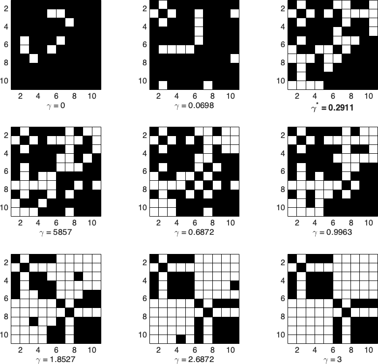
For the observed multivariate count data for , we applied Algorithm 3.1. We found values 0, 0.0698, 0.2911, 0.5857, 0.6872, 0.9963, 1.8527, 2.6891 and 3 from the trade-off curve which is given in Fig. 1. For varies values of regularization parameter on the trade off curve, the partial coherence spectrum from (43) is calculated by setting entries with to zero. Thus, all the partial coherence spectrum after thresholding corresponding to these values are given in Fig.2. We observed that sparsity has increased as we move from to . Next we rank all these partial coherence spectrum with BIC score. The BIC scores corresponding to the values are given in Fig. 3. From the Fig. 3, it is apparent that the best regularization parameter is selected to be . The estimated partial correlations and the causalities between multiple count time series corresponding to are shown in separate graphs given in Fig. 4(b) and Fig. 5(b). From the true and estimated partial correlation graphs in Fig. 4, it is observed that the proposed algorithm has misclassified only three edges as zeros and two edges as non-zeros. Similarly, from the true and estimated causality graphs Fig .5, it is seen that only four directed edges are incorrectly estimated.


5 Dengue spread in Greater Mumbai
Dengue is a viral infectious disease transmitted to humans through the bites of infected Aedes aegypti mosquitoes. It is one of the most severe health problems being faced globally. The Mumbai Metropolitan Area (previously Greater Mumbai Metropolitan Area) is divided into twenty-four administrative divisions known as wards. The dengue counts are observed weekly from January 2010 to December 2015 from the wards of Greater Mumbai by the public health department of the Municipal Corporation of Greater Mumbai (MCGM). The length of each time series is 318.
5.1 Model Estimation
In this section, we estimate the partial correlation and causality graph using the proposed Algorithm 3.1 from the observed 24-dimensional dengue data set. The time series plot of normalized dengue counts of some of the wards (A, B, and C) are shown in Fig. 6.
Remark 11.
In the plots below, the absolute counts are not shown due to data privacy rules of MCGM. However the proposed algorithm and the final results are based on the actual counts.
From these time series plots, the increasing trend and yearly seasonality with high dengue counts being reported during monsoon months are observed. The non-stationary behaviour of the dengue counts is also apparent from these plots. Thus, a linear trend and yearly seasonality represented by a pair of sine and cosine terms, are considered in the covariate vector for all wards of the model (1). Then model (1) becomes
| (45) |
where .

We estimate the unknown parameters of the model (45) and (3) with order ranging from to using Algorithm 3.1. All these models are ranked with second-order Akaike (AIC) and Bayes information criteria (BIC) which are given in Table. 1. The model of order which corresponds to the lowest AIC and BIC score is selected.
| AIC | BIC | |
|---|---|---|
| 8924.5 | 13195.8 | |
| 7176.2 | 12851.1 | |
| 7377.6 | 16530.3 | |
| 7405.1 | 19844.9 |
Thus for the model with order , we find the trade-off curve between the conditional log-likelihood () and the -type regularization function () which is shown in Fig. 7. After thresholding (see section 4.1) with threshold , the normalized inverse spectral density matrices from (43) along the trade-off curve (Fig. 7) are given in Fig. 8. We observe that sparsity pattern varies in the estimated inverse spectral density matrix from dense ( small) to diagonal ( large). We rank all of the partial correlation graphs along the trade-off curve with BIC scores which is shown in Fig. 9. The regularization parameter () values along the trade-off curve and the corresponding BIC scores are given in Table. 2. The estimated partial correlations and causalities between multiple count time series corresponding to are shown in separate graphs given in Fig.10 and Fig. 11.


| BIC | BIC | BIC | |||
|---|---|---|---|---|---|
| 0 | 12111.43 | 0.7969 | 10227.05 | 2.0186 | 10973.20 |
| 0.1706 | 10846.09 | 0.9795 | 10313.73 | 2.2213 | 11275.20 |
| 0.5084 | 10583.76 | 1.1266 | 10512.76 | 2.6271 | 11510.35 |
| 0.6829 | 10197.97 | 1.5951 | 10734.25 | 3.35 | 11811.79 |
5.2 Inference
Based on the number of undirected edges between the wards in the estimated partial correlation graph in Fig. 10, we construct a colour coded map (see Fig. 12) showing the number of incident edges for each ward. Similarly, based on the number of outward edges of each ward in the estimated causality graph of Fig. 11, we construct a colour coded map (see Fig. 13) showing the number of outgoing edges for each ward. All estimated model parameters such as undirected and directed edges for each ward along with normalized disease count (see Remark 11), are presented in the Table 3 .


The plots of the normalized dengue counts, number of undirected edges from the estimated partial correlation graph Fig. 10 and number of incoming and outgoing edges from the estimated causality graph Fig. 11 of each ward, are shown in Fig. 14. In Fig .14, all counts are normalized with their corresponding maximum.
| Ward | Count | UE | IE | OE | ||
| A | 0.252 | 0.6 | 0.411 | 0.823 | 0.508 | 0.631 |
| B | 0.217 | 0.466 | 0.529 | 0.647 | 0.369 | 0.486 |
| C | 0.201 | 0.066 | 0.176 | 0.470 | 0.202 | 0.295 |
| D | 0.278 | 0.333 | 0.411 | 0.294 | 0.343 | 0.222 |
| E | 0.984 | 0.933 | 0.764 | 0.705 | 0.799 | 0.429 |
| F/N | 0.668 | 0.8 | 0.941 | 0.529 | 0.885 | 0.307 |
| F/S | 0.481 | 0.6 | 0.647 | 0.588 | 0.624 | 0.430 |
| G/N | 0.586 | 0.866 | 0.882 | 0.705 | 0.937 | 0.567 |
| G/S | 0.964 | 0.666 | 0.647 | 0.588 | 0.727 | 0.317 |
| H/E | 1 | 0.666 | 1 | 0.470 | 1 | 0.430 |
| H/W | 0.370 | 0.533 | 0.411 | 0.411 | 0.421 | 0.354 |
| K/E | 0.365 | 0.466 | 0.529 | 0.647 | 0.584 | 0.414 |
| K/W | 0.372 | 0.466 | 0.235 | 0.764 | 0.358 | 0.477 |
| P/N | 0.607 | 0.4 | 0.647 | 0.294 | 0.718 | 0.287 |
| P/S | 0.431 | 0.266 | 0.470 | 0.411 | 0.510 | 0.276 |
| R/C | 0.352 | 0.666 | 0.705 | 0.470 | 0.695 | 0.347 |
| R/N | 0.638 | 0.533 | 0.705 | 0.705 | 0.753 | 0.425 |
| R/S | 0.521 | 0.666 | 0.529 | 0.823 | 0.639 | 0.706 |
| L | 0.522 | 1 | 0.647 | 1 | 0.766 | 1 |
| M/E | 0.261 | 0.466 | 0.294 | 0.705 | 0.318 | 0.515 |
| M/W | 0.116 | 0 | 0.058 | 0.352 | 0.143 | 0.419 |
| N | 0.379 | 0.4 | 0.588 | 0.470 | 0.602 | 0.308 |
| S | 0.608 | 0.6 | 0.882 | 0.470 | 0.862 | 0.362 |
| T | 0.272 | 0.6 | 0.705 | 0.470 | 0.573 | 0.242 |
In Fig. 15, the normalized dengue counts, number of undirected edges of each ward, total incoming weights and total outgoing weights given in (8) and (9) of each ward are shown.


Several expected and some unexpected inferences are evident from Fig. 14 and 15:
- 1.
Dengue counts in some wards (A, E, F/N, G/N, L) are highly correlated with counts in other wards. This is evident from the high number of undirected edges of the estimated partial correlation graph incident upon these wards. While this observation provides some insight into the spread pattern, information about the direction of the spread is not available.
- 2.
Some of the wards (A, R/S, L) act as sources of dengue spread. This is evident from the high number of outgoing edges of the estimated causality graph emanating from these wards.
- 3.
Actual dengue count can be low for these source wards (A, R/S, L). This is quite counter-intuitive and one of the key findings of this analysis. A very high daily commuter flow might explain this phenomenon.
- 4.
6 Conclusion
In this paper, we have investigated graphical interaction models of multivariate time series of counts using a parametric approach. The partial correlations and causalities between observed multivariate count data are defined in terms of the partial correlations and causalities between latent processes. Further a joint MLE with -type regularization is used to estimate the inverse spectral density matrix. To overcome the computational difficulties with the resulting mixture distributions, an MCEM algorithm with -type regularization is proposed. Asymptotic convergence results for the sequence generated by Algorithm 3.1 are presented and the results are verified with simulations. Finally, the partial correlation and causality graphs are estimated for dengue count data observed weekly from each ward of Greater Mumbai city over six years. Surprisingly some wards seem to act as epicenters of disease spread even though their absolute disease counts are relatively low. Such an inference may help correct public health intervention policies in the future.
acknowledgments-disclosure-of-funding.
This work was partially supported by the Science and Research Engineering Board (Department of Science and Technology, Government of India). The authors thank Municipal Corporation of Greater Mumbai (MCGM) for providing the dengue dataset.References
- Alpago et al. (2018) D. Alpago, M. Zorzi, and A. Ferrante. Identification of sparse reciprocal graphical models. IEEE Control Systems Letters, 2(4):659–664, Oct 2018. ISSN 2475-1456.
- Avventi et al. (2013) E. Avventi, A. G. Lindquist, and B. Wahlberg. Arma identification of graphical models. IEEE Transactions on Automatic Control, 58(5):1167–1178, May 2013. ISSN 0018-9286.
- Bach and Jordan (2004) Francis R. Bach and Michael I. Jordan. Learning graphical models for stationary time series. IEEE Trans. Signal Processing, 52(8):2189–2199, 2004.
- Brillinger (1981) David R. Brillinger. Time Series Data Analysis and Theory. Society for Industrial and Applied Mathematics Philadelphia, 1981.
- Brillinger (1996) David R. Brillinger. Remarks concerning graphical models for time series and point processes. Revista de Econometria, 16:1–23, 1996.
- Brockwell and Davis (2002) Peter J. Brockwell and Richard A. Davis. Introduction to Time Series and Forecasting. Springer, 2nd edition, mar 2002. ISBN 0387953515.
- Casella and Berger (2002) G. Casella and R.L. Berger. Statistical Inference. Duxbury advanced series in statistics and decision sciences. Thomson Learning, 2002. ISBN 9780534243128.
- Cawley and Talbot (2010) Gavin C. Cawley and Nicola L. C. Talbot. On over-fitting in model selection and subsequent selection bias in performance evaluation. Journal of Machine Learning Research, 11:2079–2107, 2010.
- Chan and Ledolter (1995) K. S. Chan and Johannes Ledolter. Monte carlo em estimation for time series models involving counts. Journal of the American Statistical Association, 90(429):242–252, 1995. ISSN 01621459.
- Ciccone et al. (2018) V. Ciccone, A. Ferrante, and M. Zorzi. Robust identification of “sparse plus low-rank” graphical models: An optimization approach. In 2018 IEEE Conference on Decision and Control (CDC), pages 2241–2246, Dec 2018.
- Dahlhaus (2000) R. Dahlhaus. Graphical interaction models for multivariate time series. Metrika, (51):157–172, 2000.
- Dahlhaus and Eichler (2003) Rainer Dahlhaus and Michael Eichler. Causality and graphical models in time series analysis. Oxford Stat. Sci. Ser, 27, 01 2003.
- David A. Bessler (2003) Jian Yang David A. Bessler. The structure of interdependence in international stock markets, journal of international money and finance. Journal of International Money and Finance, 22(2):261–287, 2003. ISSN 0261-5606.
- Dempster (1972) A. P. Dempster. Covariance selection. Biometrics, 28(1):157–175, 1972. ISSN 0006341X, 15410420.
- Dempster et al. (1977) Arthur Dempster, Natalie Laird, and Donald B. Rubin. Maximum likelihood from incomplete data via the em algorithm. Journal of the Royal Statistical Society. Series B (Methodological), 39:1–38, 01 1977.
- Durbin and Koopman. (2000) J. Durbin and S. J. Koopman. Time series analysis of non-gaussian observations based on state-space models from both classical and Bayesian perspectives. Journal of the Royal Statistical Society, Ser. B, 62:3–56, 2000.
- Eichler (2006) Michael Eichler. Fitting graphical interaction models to multivariate time series. Proceedings of the 22nd Conference on Uncertainty in Artificial Intelegence, 2006.
- Eichler (2007) Michael Eichler. Granger causality and path diagrams for multivariate time series. Journal of Econometrics, 137(2):334 – 353, 2007. ISSN 0304-4076.
- Eichler (2012) Michael Eichler. Graphical modelling of multivariate time series. Probability Theory and Related Fields, 153(1):233–268, Jun 2012. ISSN 1432-2064.
- Fahrmeir and Tutz (1994) L. Fahrmeir and G. Tutz. Multivariate Statistical Modelling Based on Generalized Linear Models. Springer series in statistics. Springer-Verlag, 1994. ISBN 9780387942339. URL https://books.google.co.in/books?id=OionAQAAIAAJ.
- Fahrmeir and Tutz (2001) L. Fahrmeir and G. Tutz. Multivariate Statistical Modeling Based on Generalized Linear Models. Springer-Verlag, New York, 2001.
- Fahrmeir and Wagenpfeil (1997) L. Fahrmeir and S. Wagenpfeil. Penalized likelihood estimation and iterative Kalman filtering for non-gaussian dynamic regression models. Computational Statistics and Data Analysis, 24:295–320, 1997.
- Helmut (2005) Lütkepohl Helmut. New introduction to multiple time series analysis. Springer Berlin Heidelberg, 2005.
- Hsiao (1982) Cheng Hsiao. Autoregressive modeling and causal ordering of economic variables. Journal of Economic Dynamics and Control, 4:243 – 259, 1982.
- Hue and Chiogna (2021) Nguyen Thi Kim Hue and Monica Chiogna. Structure learning of undirected graphical models for count data. Journal of Machine Learning Research, 22:50–1, 2021.
- Jung et al. (2015) A. Jung, G. Hannak, and N. Goertz. Graphical lasso based model selection for time series. IEEE Signal Processing Letters, 22(10):1781–1785, Oct 2015. ISSN 1070-9908.
- J.Z. Huang and Liu (2006) M. Pourahmadi J.Z. Huang, N. Liu and L. Liu. Covariance matrix selection and estimation via penalised normal likelihood. Biometrika, 1(93):85–98, 2006.
- Li (1994) W. K. Li. Time series models based on generalized linear models: Some further results. Biometrics, 50:506–511, 1994.
- Lounici (2008) Karim Lounici. Sup-norm convergence rate and sign concentration property of lasso and dantzig estimators. Electron. J. Statist., 2:90–102, 2008.
- McLachlan and Krishnan (2008) Geoffrey J. McLachlan and Thriyambakam Krishnan. The EM algorithm and extensions. Wiley series in probability and statistics. Wiley, Hoboken, NJ, 2. ed edition, 2008.
- Mehdi Jalalpour and Levin (2015) Yulia Gel Mehdi Jalalpour and Scott Levin. Forecasting demand for health services: development of a publicly available toolbox. Operations Research for Health Care, 5:1–9, 2015.
- Mengersen and Tweedie (1996) K. L. Mengersen and R. L. Tweedie. Rates of convergence of the hastings and metropolis algorithms. The Annals of Statistics, 24(1):101–121, 1996.
- Park and Park (2019) Gunwoong Park and Sion Park. High-dimensional poisson structural equation model learning via ell_1-regularized regression. Journal of Machine Learning Research, 20:95–1, 2019.
- Park and Raskutti (2015) Gunwoong Park and Garvesh Raskutti. Learning large-scale poisson dag models based on overdispersion scoring. Advances in neural information processing systems, 28, 2015.
- Park and Raskutti (2017) Gunwoong Park and Garvesh Raskutti. Learning quadratic variance function (qvf) dag models via overdispersion scoring (ods). Journal of Machine Learning Research, 18:224–1, 2017.
- Pierce and Haugh (1977) David A Pierce and Larry D Haugh. Causality in temporal systems: Characterization and a survey. Journal of econometrics, 5(3):265–293, 1977.
- Qian et al. (2015) Long Qian, Yi Zhang, Li Zheng, Yuqing Shang, Jia-Hong Gao, and Yijun Liu. Frequency dependent topological patterns of resting-state brain networks. PLOS ONE, 10(4):1–19, 04 2015.
- R.K.Freeland and McCabe (2004) R.K.Freeland and B.P.M. McCabe. Forecasting discrete valued low count time series. International Journal of Forecasting, 20:427–434, 2004.
- Roberts and Tweedie (1996) G. O. Roberts and R. L. Tweedie. Geometric convergence and central limit theorems for multidimensional hastings and metropolis algorithms. Biometrika, 83(1):95–110, 1996.
- Roberts and Smith (1994) G.O. Roberts and A.F.M. Smith. Simple conditions for the convergence of the gibbs sampler and metropolis-hastings algorithms. Stochastic Processes and their Applications, 49(2):207 – 216, 1994. ISSN 0304-4149.
- Roy and Dunson (2020) Arkaprava Roy and David B Dunson. Nonparametric graphical model for counts. Journal of Machine Learning Research, 21(229):1–21, 2020.
- Sathish et al. (2019) Vurukonda Sathish, Debraj Chakraborty, and Siuli Mukhopadhyay. Topology selection using monte carlo expectation and maximization algorithm with l1-type regularization for count data. pages 6977–6982, 2019.
- Sims (1972) Christopher A Sims. Money, income, and causality. The American economic review, 62(4):540–552, 1972.
- Songsiri (2010) Jitkomut Songsiri. Graphical Models of Time Series: Parameter Estimation and Topology Selection. 2010.
- Songsiri (2013) Jitkomut Songsiri. Sparse autoregressive model estimation for learning granger causality in time series. In 2013 IEEE International Conference on Acoustics, Speech and Signal Processing, pages 3198–3202. IEEE, 2013.
- Songsiri (2015) Jitkomut Songsiri. Learning multiple granger graphical models via group fused lasso. In 2015 10th Asian Control Conference (ASCC), pages 1–6. IEEE, 2015.
- Songsiri and Vandenberghe (2010) Jitkomut Songsiri and Lieven Vandenberghe. Topology selection in graphical models of autoregressive processes. J. Mach. Learn. Res., 11:2671–2705, December 2010. ISSN 1532-4435.
- Songsiri et al. (2009) Jitkomut Songsiri, Joachim Dahl, and Lieven Vandenberghe. Graphical models of autoregressive processes. Convex Optimization in Signal Processing and Communications, 01 2009. doi: 10.1017/CBO9780511804458.004.
- Tibshirani (1996) R. Tibshirani. Regression shrinkage and selection via the lasso. Journal of the Royal Statistical Society (Series B), 58:267–288, 1996.
- TjØstheim (1981) Dag TjØstheim. Granger-causality in multiple time series. Journal of Econometrics, 17(2):157 – 176, 1981.
- Utazi et al. (2018) C. Edson Utazi, Emmanuel O. Afuecheta, and C. Christopher Nnanatu. A bayesian latent process spatiotemporal regression model for areal count data. Spatial and Spatio-temporal Epidemiology, 25:25 – 37, 2018. ISSN 1877-5845.
- W. J. Granger (1969) Clive W. J. Granger. Investigating causal relations by econometric models and cross-spectral methods. Econometrica, 37:424–38, 02 1969. doi: 10.2307/1912791.
- Wei and Tanner (1990) Greg C. G. Wei and Martin A. Tanner. A monte carlo implementation of the em algorithm and the poor man’s data augmentation algorithms. Journal of the American Statistical Association, 85(411):699–704, 1990.
- Wright (1921) Sewall Wright. Correlation and causation. J. agric. Res., 20:557–580, 1921.
- Wright (1934) Sewall Wright. The method of path coefficients. The annals of mathematical statistics, 5(3):161–215, 1934.
- Zeger and Qaqish (1988) Scott L. Zeger and Bahjat Qaqish. Markov regression models for time series: A quasi-likelihood approach. Biometrics, 44(4):1019–1031, 1988.
- Zorzi and Sepulchre (2016) M. Zorzi and R. Sepulchre. Ar identification of latent-variable graphical models. IEEE Transactions on Automatic Control, 61(9):2327–2340, Sep. 2016. ISSN 0018-9286.