Animating Sand, Mud, and Snow
Abstract
Computer animations often lack the subtle environmental changes that should occur due to the actions of the characters. Squealing car tires usually leave no skid marks, airplanes rarely leave jet trails in the sky, and most runners leave no footprints. In this paper, we describe a simulation model of ground surfaces that can be deformed by the impact of rigid body models of animated characters. To demonstrate the algorithms, we show footprints made by a runner in sand, mud, and snow as well as bicycle tire tracks, a bicycle crash, and a falling runner. The shapes of the footprints in the three surfaces are quite different, but the effects were controlled through only five essentially independent parameters. To assess the realism of the resulting motion, we compare the simulated footprints to human footprints in sand.
Keywords: animation, physical simulation, ground interaction, terrain, sand, mud, snow.
1 Introduction
To become a communication medium on a par with movies, computer animations must present a rich view into an artificial world. Texture maps applied to three-dimensional models of scenery help to create some of the required visual complexity. But static scenery is only part of the answer; subtle motion of many elements of the scene is also required. Trees and bushes should move in response to the wind created by a passing car, a runner should crush the grass underfoot, and clouds should drift across the sky. While simple scenery and sparse motion can sometimes be used effectively to focus the attention of the viewer, missing or inconsistent action may also distract the viewer from the plot or intended message of the animation. One of the principles of animation is that the viewer should never be unintentionally surprised by the motion or lack of it in a scene[1].

Subtle changes in the scenery may also convey important information about the plot or scene context to the viewer. For example, figure 1 shows an image of alien bikers riding across a desert landscape. The presence of tracks makes it clear that the ground is soft sand rather than hard rock, and that other bikers have already passed through the area. Figure 2 shows the same scene without the sand. In addition to being visually less interesting, the altered image lacks some of the visual cues that help the viewer understand the scene.

Movie directors face a related problem because they must ensure that the viewer is presented with a consistent view of the world and the characters. An actor’s clothing should not inexplicably change from scene to scene, lighting should be consistent across edits, and such absent, unexpected, or anachronistic elements as missing tire tracks, extra footprints, or jet trails must be avoided. The risk of distracting the viewer is so great that one member of the director’s team, known as a “continuity girl,” “floor secretary,” or “second assistant director,” is responsible solely for maintaining consistency[2].
Maintaining consistency is both easier and harder in computer animation. Because we are creating an artificial world, we can control the lighting conditions, layout, and other scene parameters and recreate them if we need to “shoot” a fill-in scene later. Because the world is artificial, however, we may be tempted to rearrange objects between scenes for best effect, thereby creating a series of scenes that could not coexist in a consistent world. Computer-generated animations and special effects add another facet to the consistency problem because making models that move and deform appropriately is a lot of work. For example, most animated figures do not leave tracks in the environment as a human actor would and special effects artists have had to work hard to create such subtle but essential effects as environment maps of flickering flames. Because each detail of the scene represents additional work, computer graphics environments are often conspicuously clean and sparse. The approach presented here is a partial solution to this problem; we create a more interesting environment by allowing the character’s actions to change a part of the environment.
In this paper, we describe a model of ground surfaces and explain how these surfaces can be deformed by characters in an animation. The ground material is modeled as a height field formed by vertical columns. After the impact of a rigid body model, the ground material is deformed by allowing compression of the material and movement of material between the columns. To demonstrate the algorithms, we show the creation of footprints in sand, mud, and snow. These surfaces are created by modifying only five essentially independent parameters of the simulation. We evaluate the results of the animation through comparison with video footage of human runners and through more dramatic patterns created by bicycle tire tracks (figure 1), a falling bicycle (figure 7), and a tripping runner (figure 10).
2 Background
Several researchers have investigated the use of procedural techniques for generating and animating background elements in computer-generated scenes. Although we are primarily interested in techniques that allow the state of the environment to be altered in response to the motions of an actor, methods for animating or modeling a part of the environment independent of the movements of the actors are also relevant because they can be modified to simulate interactions.
The first example of animated ground tracks for computer animation was work done by Lundin[3, 4]. He describes how footprints can be created efficiently by rendering the underside of an object to create a bump map and then applying the bump map to the ground surface to create impressions where the objects have contacted the ground.
The work most closely related to ours is that of Li and Moshell[5]. They developed a model of soil that allows interactions between the soil and the blades of digging machinery. Soil spread over a terrain is modeled using a height field, and soil that is pushed in front of a bulldozer’s blade is modeled as discrete chunks. Although they discount several factors that contribute to soil behavior in favor of a more tractable model, their technique is physically based and they arrive at their simulation formulation after a detailed analysis of soil dynamics. As the authors note, actual soil dynamics is complex and their model, therefore, focuses on a specific set of actions that can be performed on the soil, namely the effect of horizontal forces acting on the soil causing displacements and soil slippage. The method we present here has obvious similarities to that of Li and Moshell, but we focus on modeling a different set of phenomena at different scales. We also adopt a more appearance-based approach in the interest of developing a technique that can be used to model a wide variety of ground materials for animation purposes.
Another method for modeling the appearance of ground surfaces is described by Chanclou, Luciani, and Habibi[6]. They use a simulation-based ground surface model that behaves essentially like an elastic sheet. The sheet deforms plasticly when acted on by other objects. While their model allows objects to make smooth impressions in the ground surface, they do not describe how their technique could be used to realistically model real world ground materials.
Nishita and his colleagues explored modeling and rendering of snow using metaballs[7]. Their approach allowed them to model snow on top of objects and drifts to the side of objects. They also developed a method for realistically rendering snow that captured effects due to multiple levels of light scattering.
Other environmental effects that have been animated include water, clouds and gases[8, 9, 10], fire[9, 11], lightning[12], and leaves blowing in the wind[13]. Among these, water has received the most attention. Early work by Peachey[14] and by Fournier and Reeves[15] used procedural models based on specially designed wave functions to model ocean waves as they travel and break on a beach. Later work by Kass and Miller[16] developed a more general approach using shallow water equations to model the behavior of water under a wider variety of conditions. Their model also modified the appearance of a sand texture as it became wet. O’Brien and Hodgins[17] extended the work of Kass and Miller to allow the behavior of the water simulation to be affected by the motion of other objects in the environment and to allow the water to affect the motion of the other objects. They included examples of objects floating on the surface and simulated humans diving into pools of water. More recently Foster and Metaxas[18] used a variation of the three-dimensional Navier-Stokes equations to model fluids. In addition to these surface and volumetric approaches, particle-based methods have been used to model water spray and other loosely packed materials. Supplementing particle models with inter-particle dynamics allows a wider range of phenomena to be modeled. Examples of these systems include Reeves[19], Sims[20], Miller and Pearce[21], and Terzopoulos, Platt, and Fleischer[22].
Simulation of interactions with the environment can also be used to generate still models. Several researchers have described techniques for generating complex plant models from grammars describing how the plant should develop or grow over time. Měch and Prusinkiewicz[23] developed techniques for allowing developing plants to affect and be affected by their environment. Dorsey and her colleagues[24, 25] used simulation to model how an object’s surface changes over time as environmental factors act on it.
3 Simulation of Sand, Mud, and Snow
In this paper, we present a general model of a deformable ground material. The model consists of a height field defined by vertical columns of material. Using displacement and compression algorithms, we animate the deformations that are created when rigid geometric objects impact the ground material and create footprints, tire tracks, or other patterns on the ground. The properties of the model can be varied to produce the behavior of different ground materials such as sand, mud, and snow.
3.1 Model of Ground Material


Our simulation model discretizes a continuous volume of ground material by dividing the surface of the volume into a uniform rectilinear grid that defines a height field (figure 3). The resolution of the grid must be chosen appropriately for the size of the desired features in the ground surface. For example, in figure 1 the resolution of the grid is 1 cm and the bicycles are approximately 2 meters long with tires 8 cm wide. Though the resolution of the grid determines the size of the smallest feature that can be represented, it does not otherwise dramatically affect the shape of the resulting terrain (figure 4).
Initial conditions for the height of each grid point can be created procedurally or imported from a variety of sources. We implemented initial conditions with noise generated on an integer lattice and interpolated with cubic Catmull-Rom splines (a variation of a two-dimensional Perlin noise function described by Ebert[8]). Terrain data or the output from a modeling program could also be used for the initial height field. Alternatively, the initial conditions could be the output of a previous simulation run. For example, the trampled surface of a public beach at the end of a busy summer day could be modeled by simulating many crisscrossing paths of footprints.
3.2 Motion of the Ground Material

The height field represented by the top of the columns is deformed as rigid geometric objects push into the grid. For the examples given in this paper, the geometric objects are a runner’s shoe, a bicycle tire and frame, and a jointed human figure. The motion of the rigid bodies was computed using a dynamic simulation of a human running, bicycling, or falling down on a smooth, hard ground plane[26]. The resulting motion was given as input to the simulation of the ground material in the form of trajectories of positions and orientations of the geometric objects. Because of this generic specification of the motion, the input motion need not be dynamically simulated but could be keyframe or motion capture data.
The surface simulation approximates the motion of the columns of ground material by compressing or displacing the material under the rigid geometric objects. At each time step, a test is performed to determine whether any of the rigid objects have intersected the height field. The height of the affected columns is reduced until they no longer penetrate the surface of the rigid object. The material that was displaced is either compressed or forced outward to surrounding columns. A series of erosion steps are then performed to reduce the magnitude of the slopes between neighboring columns. Finally, particles can be generated from the contacting surface of the rigid object to mimic the spray of material that is often seen following an impact. These stages are illustrated in figure 5. We now discuss each stage of the algorithm in more detail: collision, displacement, erosion, and particle generation.
Collision.
The collision detection and response algorithm determines whether a rigid object has collided with the ground surface. For each column, a ray is cast from the bottom of the column through the vertex at the top. If the ray intersects a rigid object before it hits the vertex, then the rigid object has penetrated the surface and the top of the column is moved down to the intersection point. A flag is set to indicate that the column was moved, and the change in height is recorded. The computational costs of the ray intersection tests are reduced by partitioning the polygons of the rigid body models using an axis-aligned bounding box hierarchy[27].
Using a vertex coloring algorithm, the simulation computes a contour map based on the distance from each column that has collided with the object to the closest column that has not collided (figure 6). This information is used when the material displaced by the collision is distributed. As an initialization step, columns not in contact with the object are assigned the value zero. During subsequent iterations, unlabeled columns adjacent to labeled columns are assigned a value equal to the value of the lowest numbered adjacent column plus one.
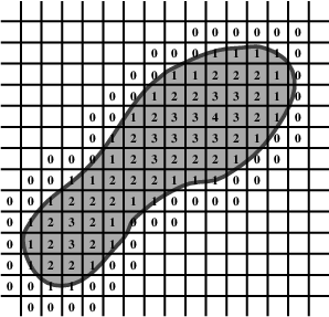
Displacement.
Ground material from the columns that are in contact with the object is either compressed or distributed to surrounding columns that are not in contact with the object. The compression ratio is chosen by the user and is one of the parameters available for controlling the visual appearance of the ground material. The material to be distributed, , is computed by , where is the total amount of displaced material. The material that is not compressed is equally distributed among the neighbors with lower contour values, so that the ground material is redistributed to the closest ring of columns not in contact with the rigid object. The heights of the columns in this ring are increased to reflect the newly deposited material.
Erosion.
Because the displacement algorithm deposits material only in the first ring of columns not in contact with the object, the heights of these columns may be increased in an unrealistic fashion. An “erosion” algorithm is used to identify columns that form steep slopes with their neighbors and move material down the slope to form a more realistic mound. Several parameters allow the user to control the shape of the mound and model different ground materials.
The erosion algorithm examines the slope between each pair of adjacent columns in the grid. For a column and a neighboring column , the slope, , is
| (1) |
where is the height of column and is the distance between the two columns. If the slope between two neighboring columns is greater than a threshold , then ground material is moved from the higher column down the slope to the lower column. In the special case where one of the columns is in contact with the geometric object, a different threshold, , is used to provide independent control of the inner slope. Ground material is moved by computing the average difference in height, , for the neighboring columns with too large a downhill slope:
| (2) |
The average difference in height is multiplied by a fractional constant, , and the resulting quantity is equally distributed among the downhill neighbors. This step in the algorithm repeats until all slopes are below a threshold, . The erosion algorithm may cause some columns to intersect a rigid object but this penetration will be corrected on the next time step.


Particle Generation.
We use a particle system to model portions of the ground material that are thrown into the air by the motion of the rigid geometric objects. The user controls the adhesiveness between the object and the material as well as the rate at which the particles fall from the object. Each triangle of the object that is in contact with the ground picks up a volume of the ground material during contact. The volume of material is determined by the area of the triangle multiplied by an adhesion constant for the material. When the triangle is no longer in contact with the ground, it drops the attached material as particles according to an exponential decay rate.
| (3) |
where is the initial volume attached to the triangle, is the current time, is the time at which the triangle left the ground, is the time step size, and is a half life parameter that controls how quickly the material falls off. The number of particles released on a given time step is determined by , where is the volume of each particle.
The initial position, , for a particle is randomly distributed over the surface of the triangle according to:
| (4) |
where , , and are the coordinates of the vertices of the triangle and , , and are the barycentric coordinates of given by
| (5) | |||||
| (6) | |||||
| (7) |
where and are independent random variables evenly distributed between . This computation results in a uniform distribution over the triangle[28].
The initial velocity of a particle is computed from the velocity of the rigid object:
| (8) |
where and are the linear and angular velocity of the object. To give a more realistic and appealing look to the particle motion, the initial velocities are randomly perturbed.
The final component of the particle creation algorithm accounts for the greater probability that material will fall off rapidly accelerating objects. A particle is only created if , where is the minimal acceleration at which all potential particles will be dropped, controls the variation of the probability of particle creation with speed, and is a random variable evenly distributed in the range .
If particles are only generated at the beginning of a time step then the resulting particle distribution will have a discrete, sheetlike appearance. We avoid this undesirable effect by randomly distributing each particle’s creation time within the time step interval. The information used to calculate the initial position and velocity is interpolated within the interval to obtain information appropriate for the particle’s creation time.
Once generated, the particles fall under the influence of gravity. When a particle hits the surface of a column, its volume is added to the column.
3.3 Implementation and Optimization
Simulations of terrain generally span a large area. For example, we would like to be able to simulate a runner jogging on a beach, a skier gliding down a snow-covered slope, and a stampede of animals crossing a sandy valley. A naive implementation of the entire terrain would be intractable because of the memory and computation requirements. The next two sections describe optimizations that allow us to achieve reasonable performance by storing and simulating only the active portions of the surface and by parallelizing the computation.
Algorithm Complexity.
Because the ground model is a two-dimensional rectilinear grid, the most straightforward implementation is a two-dimensional array of nodes containing the height and other information about the column. If an animation required a grid of rows and columns, nodes would be needed, and computation time and memory would grow linearly with the number of grid points. Thus, a patch of ground 10 m 10 m with a grid resolution of 1 cm yields a grid with one million nodes. If each node requires 10 bytes of memory, the entire grid requires 10 Mbytes of storage. Even this relatively small patch of ground requires significant system resources. However, most of the ground nodes are static throughout the simulation, allowing us to use a much more efficient algorithm that creates and simulates only the active nodes.
The active area of the ground surface is determined by projecting an enlarged bounding box for the rigid objects onto the surface as shown in figure 7. The nodes within the projection are marked as active, and the collision detection, displacement, and erosion algorithms are applied, not to the entire grid, but only to these active grid points. Additionally, nodes are not allocated for the entire ground surface, rather they are created on demand as they become active. The position of a particular node is used as the index into a hash table allowing the algorithms to be implemented as if a simple array of nodes were being used.
Because only the active grid points are processed, the computation time is now a function of the size of the rigid objects in the scene rather than the total grid size. Memory requirements are also significantly reduced, although the state of all modified nodes must be stored even after they are no longer active.

Parallel Implementation.
Despite the optimization provided by simulating only active nodes, the computation time grows linearly with the projected area of the rigid objects. Adding a second character will approximately double the active area (see figure 8), but the computation time for multiple characters can be reduced by using parallel processing when the characters are contacting independent patches of ground.
We have designed and implemented a parallel scheme for the ground surface simulation. A single parent process maintains the state of the grid and coordinates the actions of the child processes. During initialization, a child process is created for each character that will interact with the ground surface. The children communicate with the parent process via the UNIX socket mechanism and may exist together on a single multiprocessor machine or on several separate single processor machines.
Each child computes the changes to the grid caused by its character as quickly as possible, without any direct knowledge about the progress of the other children. When a child completes the computation for a time step, it reports the changes it has made to the parent process and then waits for information about any new grid cells that will be in the bounding box for its character during the next time step. However, if the child is ready to compute a time step before another child has reported prior changes that are within the bounding box of a character assigned to the first child, the parent will prevent the first child from continuing until the changes are available. For example, in an animation of a cyclist that rides across a footprint left by a runner, the child process computing the cyclist may arrive at the footprint location before the process computing the runner has simulated the creation of the footprint. If two or more characters have overlapping bounding boxes for the same time step, the computation for those characters is reassigned to a single child process until they no longer overlap.


Simulation run times for both the serial and parallel versions of our algorithm are shown in figure 8. As expected, the time required by the serial implementation grows linearly with the number of characters. Ideally, the time required by the parallel implementation would be constant since each character has its own processor. However, due to communication overhead and interactions between the characters, the run time for the parallel version grows as the number of characters increases, but at a much slower rate than the serial version.
4 Animation Parameters
One goal of this research is to create a tool that allows animators to easily generate a significant fraction of the variety seen in ground materials. Five parameters of the simulation can be changed by the user to achieve different effects: inside slope, outside slope, roughness, liquidity, and compression. The first four are used by the erosion algorithm, and the fifth is used by the displacement algorithm.
The inside and outside slope parameters, and , modify the shape of a mound of ground material by changing the slope adjacent to intersecting geometry and the slope on the outer part of the mound. Small values lead to more erosion and a more gradual slope; large values yield less erosion and a steeper slope.
Roughness, , controls the irregularity of the ground deformations by changing the amount of material that is moved from one column to another during erosion. Small values yield a smooth mound of material while larger values give a rough, irregular surface.
Liquidity, , determines how watery the material appears by controlling the amount of erosion within a single timestep. With less erosion per time step, the surface appears to flow outward from the intersecting object; with more erosion, the surface moves to its final state more quickly.
The compression parameter, , offers a way to model substances of different densities by determining how much displaced material is distributed outward from an object that has intersected the grid. A value of one causes all material to be displaced; a value less than one allows some of the material to be compressed.
When particles are used, additional parameters are required to determine their appearance. We included parameters to control adhesion, particle size, and the rate at which material falls off of the objects. We used particles in the animations of sand but did not include them in the animations of mud or snow. Other more dynamic motions such as skiing might generate significant spray, but running in snow appears to generate clumps of snow rather than particles.
5 Results and Discussion
| Effect | Variable | Sand | Mud | Snow |
|---|---|---|---|---|
| inside slope | 0.8 | 1.57 | 1.57 | |
| outside slope | 0.436 | 1.1 | 1.57 | |
| roughness | 0.2 | 0.2 | 0.2 | |
| liquidity | 0.8 | 1.1 | 1.57 | |
| compression | 0.3 | 0.41 | 0.0 |
Figure 9 shows images of a human runner stepping in sand and a simulated runner stepping in sand, mud, and snow. The parameters used for the simulations of the three ground materials are given in table 1. The footprints left by the real and simulated runners in sand are quite similar.
Figures 7 and 10 show more complicated patterns created in the sand by a falling bicycle and a tripping runner. For each of these simulations, we used a grid resolution of 1 cm by 1 cm yielding a virtual grid size of 20481024 for the bicycle and 4096512 for the runner.
The images in this paper were rendered with Pixar’s RenderMan software. We found that rendering the ground surface using a polygonal mesh was computationally expensive and that the data files required to describe the mesh were large and difficult to work with. We achieved better results using a single polygon with a displacement shader that modeled the ground surface.
The simulation described in this paper allows us to capture many of the behaviors of substances such as sand, mud, and snow. Only about fifteen iterations were required to hand tune the parameters for the desired effect with each material. The computation time is not burdensome: a 3-second simulation of the running figure interacting with a 1 cm by 1 cm resolution ground material required less than 2 minutes of computation time on a single MHz MIPS R10000 processor.
Many effects are missed by this model. For example, wet sand and crusty mud often crack and form large clumps, but our model can generate only smooth surfaces and particles. Actual ground material is not uniform but contains both small grains of sand or dirt as well as larger objects such as rocks, leaves, and sea shells. More generally, many factors go into creating the appearance of a given patch of ground: water and wind erosion, plant growth, and the footprints of many people and animals. Some of these more subtle effects are illustrated by the human footprints in snow and mud shown in figure 11.

One significant approximation in the ground simulation is that the motion of the rigid objects is not affected by the deformations of the surface. For the sequences presented here, each of the rigid body simulations interacted with a flat, smooth ground plane. A more accurate and realistic simulation would allow the bike and runner to experience the undulations in the initial terrain as well as the changes in friction caused by the deforming surfaces. For example, a bike is slowed down significantly when rolling on sand and a runner’s foot slips slightly with each step on soft ground.
Other approximations are present in the way that the sand responds to the motion of the rigid objects. For example, a given area of sand has no memory of the compression caused by previous impacts. Because the motion of the rigid objects are specified in advance, this approximation does not cause any noticeable artifacts. Compression could also be used to change rendering parameters as appropriate.
We do not take the velocity of the rigid object into account in the ground simulation. For bicycling and running, this approximation is negligible because the velocities of the wheel and the foot with respect to the ground are small at impact. For the falling runner or bicycle, however, this approximation means that the ridge of sand is uniformly distributed rather than forming a larger ridge in the direction of travel.
The motions of sand, mud, and snow that we generated are distinctly different from each other because of changes to the simulation parameters. Although much of the difference is due to the deformations determined by our simulations, part of the visual difference results from different surface properties used for rendering. To generate the images in this paper, we had not only to select appropriate parameters for the simulation but also to select parameters for rendering. A more complete investigation of techniques for selecting rendering parameters and texture maps might prove useful.
We regard this simulation as appearance-based rather than engineering-based because most of the parameters bear only a scant resemblance to the physical parameters of the material being modeled. The liquidity parameter, for example, varies between and rather than representing the quantity of water in a given amount of sand. It is our hope that this representation for the parameters allows for intuitive adjustment of the resulting animation without requiring a deep understanding of the simulation algorithms or soil mechanics. The evaluation is also qualitative or appearance-based in that we compare simulated and video images of the footprints rather than matching initial and final conditions quantitatively.
Acknowledgments
A previous version of this paper appeared in The Proceedings of Graphics Interface ’98.
This project was supported in part by NSF NYI Grant No. IRI-9457621 and associated REU funding, Mitsubishi Electric Research Laboratory, and a Packard Fellowship. The second author was supported by an Intel Fellowship.
References
- 1. F. Thomas and O. Johnston, Disney Animation: The Illusion of Life. New York: Abbeville Press, (1984).
- 2. K. Reisz and G. Millar, The Technique of Film Editing. Focal Press, (1989).
- 3. D. Lundin, “Motion simulation”, in Nicograph ’84, (Nov. 1984).
- 4. D. Lundin, “Works’ ant”, in SIGGRAPH Video Review, vol. 100, ACM SIGGRAPH, (1994). Special Issue: Fifteen Years of Computer Graphics 1979–1994.
- 5. X. Li and J. M. Moshell, “Modeling soil: Realtime dynamic models for soil slippage and manipulation”, in SIGGRAPH ’93 Conference Proceedings, pp. 361–368, ACM SIGGRAPH, (1993).
- 6. B. Chanclou, A. Luciani, and A. Habibi, “Physical models of loose soils dynamically marked by a moving object”, in Computer Animation ’96, pp. 27–35, (1996).
- 7. T. Nishita, H. Iwasaki, and E. Nakamae, “A modeling and rendering method for snow by using metaballs”, Computer Graphics Forum, 16(3), pp. 357–364 (1997).
- 8. D. Ebert, K. Musgrave, D. Peachey, K. Perlin, and S.Worley, Texturing and Modeling: A Procedural Approach. New York: Academic Press, (Oct. 1994).
- 9. J. Stam and E. Fiume, “Depicting fire and other gaseous phenomena using diffusion processes”, in SIGGRAPH ’95 Conference Proceedings, pp. 129–136, ACM SIGGRAPH, (1995).
- 10. N. Foster and D. Metaxas, “Modeling the motion of a hot, turbulent gas”, in SIGGRAPH ’97 Conference Proceedings, pp. 181–189, ACM SIGGRAPH, (1997).
- 11. N. Chiba, S. Ohkawa, K. Muraoka, and M. Miura, “Two–dimensional visual simulation of flames, smoke and the spread of fire”, The Journal of Visualization and Computer Animation, 5(1), pp. 37–54 (1994).
- 12. T. Reed and B. Wyvill, “Visual simulation of lightning”, in SIGGRAPH ’94 Conference Proceedings, pp. 359–364, ACM SIGGRAPH, (1994).
- 13. J. Wejchert and D. Haumann, “Animation aerodynamics”, in SIGGRAPH ’91 Conference Proceedings, pp. 19–22, ACM SIGGRAPH, (1991).
- 14. D. R. Peachey, “Modeling waves and surf”, in SIGGRAPH ’86 Conference Proceedings, pp. 65–74, ACM SIGGRAPH, (1986).
- 15. A. Fournier and W. T. Reeves, “A simple model of ocean waves”, in SIGGRAPH ’86 Conference Proceedings, pp. 75–84, ACM SIGGRAPH, (1986).
- 16. M. Kass and G. Miller, “Rapid, stable fluid dynamics for computer graphics”, in SIGGRAPH ’90 Conference Proceedings, pp. 49–57, ACM SIGGRAPH, (1990).
- 17. J. F. O’Brien and J. K. Hodgins, “Dynamic simulation of splashing fluids”, in Computer Animation ’95, pp. 198–205, (1995).
- 18. N. Foster and D. Metaxas, “Realistic animation of liquids”, in Proceedings of Graphics Interface ’96, pp. 204–212, (1996).
- 19. W. T. Reeves, “Particle systems–a technique for modeling a class of fuzzy objects”, ACM Transactions on Graphics, 2, pp. 91–108 (1983).
- 20. K. Sims, “Particle animation and rendering using data parallel computation”, in SIGGRAPH ’90 Conference Proceedings, pp. 405–413, ACM SIGGRAPH, (1990).
- 21. G. Miller and A. Pearce, “Globular dynamics: A connected particle system for animating viscous fluids”, Computers and Graphics, 13(3), pp. 305–309 (1989).
- 22. D. Terzopoulos, J. Platt, and K. Fleischer, “Heating and melting deformable models (from goop to glop)”, in Proceedings of Graphics Interface ’89, pp. 219–226, (1989).
- 23. R. Měch and P. Prusinkiewicz, “Visual models of plants interacting with their environment”, in SIGGRAPH ’96 Conference Proceedings, pp. 397–410, ACM SIGGRAPH, (1996).
- 24. J. Dorsey and P. Hanrahan, “Modeling and rendering of metallic patinas”, in SIGGRAPH ’96 Conference Proceedings, pp. 387–396, ACM SIGGRAPH, (1996).
- 25. J. Dorsey, H. K. Pedersen, and P. Hanrahan, “Flow and changes in appearance”, in SIGGRAPH ’96 Conference Proceedings, pp. 411–420, ACM SIGGRAPH, (1996).
- 26. J. K. Hodgins, W. L. Wooten, D. C. Brogan, and J. F. O’Brien, “Animating human athletics”, in SIGGRAPH ’95 Conference Proceedings, pp. 71–78, ACM SIGGRAPH, (1995).
- 27. J. Snyder, “An interactive tool for placing curved surfaces without interpenetration”, in SIGGRAPH ’95 Conference Proceedings, pp. 209–218, ACM SIGGRAPH, (1995).
- 28. G. Turk, Generating Random Points in Triangles, vol. I of Graphics Gems, pp. 24–29. New York, NY: Academic Press, (1990).