High-fidelity reaction kinetic modeling of hot-Jupiter atmospheres incorporating thermal and UV photochemistry enhanced by metastable CO(a3)
Abstract
A detailed modeling of simultaneous UV-photochemical and thermochemical processes in exoplanet atmosphere-like conditions is essential for the analysis and interpretation of a vast amount of current and future spectral data from exoplanets. However, a detailed reaction kinetic model that incorporates both UV photochemistry and thermal chemistry is challenging due to the massive size of the chemical system as well as to the lack of understanding of photochemistry compared to thermal-only chemistry. Here, we utilize an automatic chemical reaction mechanism generator to build a high-fidelity thermochemical reaction kinetic model later then incorporated with UV-photochemistry enhanced by metastable triplet-state carbon monoxide (a3). Our model results show that two different photochemical reactions driven by Lyman- photons (i.e. + CO(a3) H + HCO and CO(X1) + CO(a3) C(3P) + ) can enhance thermal chemistry resulting in significant increases in the formation of , , and in -dominated systems with trace amounts of CO, which qualitatively matches with the observations from previous experimental studies. Our model also suggests that at temperatures above 2000 K, thermal chemistry becomes the dominant process. Finally, the chemistry simulated up to 2500 K does not produce any larger species such as species, benzene or larger (i.e. PAHs). This might indicate that the photochemistry of species such as might play a key role in the formation of organic aerosols observed in the previous experimental study.
Keywords:
Exoplanet atmospheres (487) — Exoplanet atmospheric composition (2021) — Planetary atmospheres (1244) — Theoretical models (2107) — Hot Jupiters (753)I Introduction
With increasing detection of exoplanets and spectroscopic characterization of exoplanet atmospheres, our knowledge of other stellar systems and planets around these stars is expanding significantly. Many of the spectral exoplanet transmission data are from the atmosphere of hot Jupiters and giant planets with short orbital periods and small semi-major axis value, which indicates that both thermal equilibrium chemistry and UV photochemistry are available in these hot-Jupiter atmospheres (Moses 2014; Madhusudhan et al. 2016), and hence simultaneous thermal and photochemical reaction pathways need to be considered when it comes to modeling the atmospheric composition of these UV-rich hot-Jupiter like exoplanets. It has been suggested from previous theoretical studies that thermal chemistry mainly dominates hot-Jupiter atmospheres with temperatures above 1500 K, while disequilibrium chemistry such as photochemistry could play an important role in exoplanet atmospheres whose temperatures are lower than 1500 K (Moses et al. 2011; Venot et al. 2012; Moses 2014).
The chemistry of an exoplanetary atmosphere largely depends on its C/O ratio, where C/O 1 indicates a carbon-rich atmosphere and C/O 1 indicates an oxygen-rich atmosphere (Solar C/O = 0.5). Along with temperature, these C/O ratios can be used to classify exoplanetary atmospheres and identify the major chemistry products that occur in each case. Several groups have explored the connection between C/O ratio, temperature, and chemistry in the hot-Jupiter atmospheres using modeling, observations, and experiments, including Madhusudhan 2012; Moses et al. 2013; Venot et al. 2015; Drummond et al. 2019 and Fleury et al. 2019; Fleury et al. 2020. Madhusudhan 2012 combined observations with an atmospheric chemical model (photochemistry not included) to classify how the C/O ratio affects the chemical compositions of the atmospheres, and Venot et al. 2015 have explored with a 1D thermo-photochemical model how various parameters including the C/O ratio affect the chemistry in hot-Jupiter atmospheres. In Fleury et al. 2019; Fleury et al. 2020, they have experimentally explored the influence of the C/O ratio on the formation of trace species and photochemical aerosols in hot-Jupiter atmospheres.
Among these, the experimental studies by Fleury et al. 2019; Fleury et al. 2020 clearly showed enhanced formation of , , and through simultaneous thermal- and UV photochemistry compared to the product formation with thermal-only chemistry at the temperature conditions below 1500 K. They also observed the formation of non-volatile hydrocarbon aerosols as solid thin films after the UV irradiation of carbon-enriched (C/O = 1) gas mixture at the temperature of 1473 K (Fleury et al. 2019).
These two previous experimental studies provided us with new and first experimental insights into potential importance of photochemistry in hot-Jupiter-like exoplanet atmospheres as well as interesting questions with regard to the formation pathways for both observed gaseous products (i.e. , , and ) and aerosol products. By tracking these formation pathways for both gaseous and condensed phase products from laboratory experimental data points, we can identify key chemical species including intermediates that are formed during UV irradiation of the laboratory analogs of exoplanet atmospheres. Eventually, these reactions can be implemented into 1D T-P profile supported atmospheric photochemical models (also known as atmospheric photochemical models) that address various physical (e.g. vertical diffusion of molecules, dry and wet deposition, atmospheric escape, condensation and sedimentation of species, etc.) and chemical (e.g. photochemistry, kinetics of the reactions between atmospheric components, etc.) principles (Hu et al. 2012). Adding a more complete picture of reaction chemistry into this atmospheric photochemical model will benefit analysis and interpretation of a vast amount of current and future spectral data from exoplanets as well as designing future space missions.
For example, the combination between the recent observational data of the atmosphere of WASP-39b by the James Webb Space Telescope (JWST) and the atmospheric chemical modeling works has suggested the first evidence of photochemistry in an exoplanet atmosphere (Tsai et al. 2022). Indeed, the JWST observational data of the atmosphere of WASP-39b shows a peak at 4.05 m which has been attributed to molecules. Using multiple atmospheric photochemical model results, Tsai et al. 2022 strongly suggest that is formed by photochemistry in the atmosphere of WASP-39b after tracking its formation pathways using reaction kinetic modeling. Therefore, it is clear that photochemistry plays an important role in the composition and spectra of observed exoplanet atmospheres, which gives a rationale that precise reaction kinetic modeling is essential when it comes to atmospheric photochemical modeling. When this precise reaction kinetic modeling is coupled with experimental work as presented in this study, it can significantly benefit the astronomical community by decreasing uncertainties in chemical reactions that need to be implemented in atmospheric chemical models used to interpret observational data.
Tracking chemical formation pathways of laboratory experiments is very challenging without the aid of reaction kinetic modeling. This is because the timescales of the initial chemical reactions are too short even for the well-controlled pseudo-first order radical chemistry (e.g. 30 s) (Golan et al. 2013), so that the products that are observed in gas-phase static cell experiments (e.g. Fleury et al. 2019; Fleury et al. 2020) are formed far beyond tertiary or even further reaction chemistry (including surface chemistry on the wall). For this reason, reaction kinetic modeling has been actively utilized in a variety of fields (e.g. astrochemistry, combustion research, etc.) to interpret various observational and experimental data. Particularly, the advancement of computer-aided automatic construction of reaction kinetic modeling in combustion research is impressive. For example, Liu et al. 2020 used Reaction Mechanism Generator (RMG, Gao et al. 2016; Liu et al. 2021) to automatically construct the acetylene pyrolysis model (with a temperature range of 1000–1500 K, a pressure of 0.2 atm, and a reaction time of 0.5 s) that contains 1594 species and 8924 reactions and successfully described up to pyrene formations observed from the previous acetylene () pyrolysis experiment by Norinaga et al. 2008.
RMG is an open-source software that automatically constructs networks with relevant core reactions based on its own algorithm to choose reaction rates (e.g. experimentally measured rates would be prioritized followed by less reliable sources in order) and a rate-based iterative algorithm for model generation (Gao et al. 2016). This approach has a few advantages over the traditional way (i.e. manually choosing reaction rates from previous references) of building reaction chemical networks: (i) since reaction rates are chosen based on a rate-based iterative algorithm, compared to manually selecting reaction rates, it is less likely that the reaction mechanism will miss important (i.e. relevant) reactions as long as the reaction libraries are solid, (ii) the approach has multiple self-feed back and refinement steps that are based on a solid algorithm, thus providing the model with more reliability, and (iii) this automatic approach enables us to describe larger and more complex chemical system that cannot be constructed by the traditional way.
As we can see from Liu et al. 2020’s pyrolysis model, in order to reasonably describe the chemistry of exoplanet atmosphere-like conditions (i.e. T = 1000–1500 K and P = 0.2 atm) with even relatively simple starting material (i.e. ), it requires a model size that is too enormous to construct manually. This enormous model size gives us a rationale to utilize this computer-aided modeling technique to precisely interpret experimental studies of hot-Jupiter atmospheric chemistry.
On top of this, including photochemistry into reaction kinetic modeling is also important. Although the temperature, pressure, and chemical conditions of hot-Jupiter atmospheres are similar to those of flame (i.e. combustion), the existence of UV photons (mainly Lyman- from their parent stars) in hot-Jupiter atmospheres is the major difference that distinguishes hot-Jupiter atmosphere from combustions (France et al. 2013; Miguel et al. 2015). Molecules in the top layers of the hot-Jupiter atmospheres will interact with accessible UV-photons and contribute to whole reaction chemistry of the system. Among a variety of molecules available in hot-Jupiter atmospheres, carbon monoxide (CO) is one of major interest to astrochemists since CO is predicted to be one of the most abundant species in hot-Jupiter-type exoplanet atmospheres whose temperatures are higher than 1000 K (Moses et al. 2013; Venot et al. 2015; Drummond et al. 2019).
In addition to this, the recent laboratory experimental results by Fleury et al. 2019; Fleury et al. 2020 strongly suggest CO as a possible photochemical precursor driven by CO photoexcitation, but lacked a detailed reaction kinetic model to explain reaction pathways to the observed products. Indeed, CO can be electronically excited to stay chemically reactive with a relatively long-lifetime through UV irradiation (Fournier et al. 1980; Gudipati & Kalb 1998; Lee et al. 2020). Although photochemically excited CO has been raised as an important precursor to photochemical pathways (Fleury et al. 2019; Roudier et al. 2021), as far as we know, no previous study has ever assessed the reaction kinetic role of this electronically excited CO in these hot-Jupiter-like atmospheres in detail.
With this background, in this paper, we will utilize an automatic chemical reaction mechanism generator to build a high-fidelity chemical network that can assess the chemical importance of photoexcited carbon monoxide and qualitatively rationalize the increase of the production yields of , , , and aerosols during UV irradiation compared to thermal-only chemistry, which were observed in the previous studies by Fleury et al. 2019; Fleury et al. 2020. Our work reported here is the first of its kind to incorporate simultaneous thermally and photochemically excited CO-induced chemical reaction pathways, which will provide not only a better insight into reaction mechanisms in hot-Jupiter like exoplanet atmospheres, but also provide a tool to confidently predict major and minor atmospheric molecular species under different conditions.
II Methods
II.1 Kinetic and thermodynamic parameter libraries
In order to consider the conversion of carbon monoxide into methane, a part of kinetic and thermodynamic parameters were taken from a recent experiment and kinetic modeling combined study of methane oxidation by Hashemi et al. 2016 and chosen as the seed mechanism’s kinetic parameters that are included in the reaction kinetic model as main chemistry. All the other kinetic and thermodynamic parameters were taken from the libraries included in the previous acetylene pyrolysis model by Liu et al. 2020 that successfully described up to pyrene (4-ring polycyclic aromatic hydrocarbons) formation observed from the previous experiment by Norinaga et al. 2008 starting from acetylene for the residence time of 0.5 s at the temperatures of 1073–1373 K, at the pressure of 80 mbar. In doing so, we can describe any larger molecules that might have been formed but not observed in the previous experiments by Fleury et al. 2019 and Fleury et al. 2020. All these kinetic and thermodynamic parameters can be found in CHEMKIN format in the Supplementary Materials. With regard to thermodynamic parameters of the triplet carbon monoxide (i.e. CO(a3)) that is not available in the library (since RMG’s library usually contains the thermodynamic parameters of molecules in the ground state), we first carried out electronic structure calculations at the CBS-QB3 level of theory using Gaussian 09 (Frisch et al. 2009) to determine geometric conformations, energies, and vibrational frequencies of the triplet carbon monoxide. Then the thermodynamic parameters of this molecule were calculated by Arkane (Allen et al. 2012), a package included in the open-source software RMG v3.1.0 (Gao et al. 2016; Liu et al. 2021), with atomic energy corrections, bond corrections, and spin orbit corrections, based on the CBS-QB3 level of theory as the model chemistry. These thermodynamic parameters of the triplet carbon monoxide is given in CHEMKIN format in the Supplementary Materials as well as molecular parameter outputs (Gaussian 09 output file) and Arkane input file.
II.2 Automoatic thermochemical reaction model generation
RMG was used to generate the thermal chemistry model that can simulate the experiments of Fleury et al. 2019; Fleury et al. 2020. An initial molar composition of 99.7 % of hydrogen and 0.3 % of carbon monoxide was used for the experimental condition of Fleury et al. 2019, while an initial molar composition of 99.26 % of hydrogen, 0.26 % of carbon monoxide, and 0.48 % of water was used for the experimental condition of Fleury et al. 2020. Batch reactor conditions were set with a temperature range of 300–1800 K and a pressure of 15 mbar for both models. These physical conditions are relevant to the atmosphere of hot Jupiters and gas giant exoplanets. For example, according to Tsai et al. 2022, the temperature profile of the atmosphere of WASP-39b (which is a hot-Jupiter type exoplanet) at 10 mbar ranges from 700 K to 1300 K, which is very similar to the physical conditions simulated in this study.
The pressure dependence feature of RMG was enabled to automatically construct pressure-dependent networks for species with up to 10 heavy atoms. Species constraints were set to limit the maximum number of carbon atoms in any molecule to 16 and the maximum number of radicals to 3 in order to keep the model generation realistic but conserve computing time as well. After the model generation completed, the final model contained 475 species and 1284 reactions (forward-reverse reaction pairs), which can be found in the Supplementary Materials as well as the RMG input file.
II.3 Rate coefficients of photochemical reactions and phosphorescence quenching of CO(a3)
Since RMG has been developed to simulate the combustion chemistry, it doesn’t include any photochemical reactions in its library. However, it is essential to include photochemical reactions in order to assess the importance of CO photochemistry in the reaction kinetic model. For this reason, we selectively calculated photochemical reaction rate coefficients (kj) of major species (that were observed in the previous experiments) as a function of the path length (l) and wavelength () under a given experimental total gas pressure (i.e. 15 mbar in Fleury et al. 2019; Fleury et al. 2020):
| (1) |
where i represents each gas species (i.e. CO, , , , or ), is the quantum yield of the photochemical reaction j, i is the photoabsorption cross-sections of the gas species i (see Figure 1c), and F0() is a photon flux at the wavelength at the photochemical reaction cell window (i.e. l=0 or zero optical depth). Unfortunately, the exact VUV photon flux, F0() profile used in the experiments conducted by Fleury et al. 2019; Fleury et al. 2020 was not available. So instead, F0() profile was taken from Ligterink et al. 2015 which used F-type microwave discharge hydrogen-flow lamps (MDHLs) similar to the system used in the previous experiments and scaled down for input power of 70 W (simulating stellar UV photons) instead of 100 W, and -pressure of 1.2 mbar instead of 0.41 mbar (refer to Fig. 4 in Ligterink et al. 2015). The resulting VUV spectra is shown in Figure 1a. The exponential term is to consider the optical depth caused by the gas species absorbing photons emitted from the UV light source, where ni is the number density of corresponding gas species i. As shown in Figure 1b, under the experimental condition of 99.7 % and 0.3 % of CO, 15 mbar, and 1473 K, at least more than 40 % of Ly- photons are available even at the end of the path length (i.e. l = 48 cm). This Equation (1) is then integrated to the photochemical cell length (i.e. l = 0 to 48 cm) as shown in Figure 1d, followed by integration to the wavelength range (i.e. = 112 to 180 nm) to calculate corresponding photochemical reaction rate coefficient (kj) as listed in Table 1.
A few assumptions have been made with respect to calculating the carbon monoxide photoexcitation (i.e. X1 a3) rate coefficient and phosphorescence (i.e. a3 X1; note that there is a spin change) rate coefficient, which are: (i) every carbon monoxide molecule in the ground state (X1) populates to a3 after UV photoexcitation into the spin and dipole allowed A1 state; (ii) phosphorescence of CO(a3) down to the ground state CO(X1) follows an exponential decay pattern determined by the radiative lifetime of the a3 state; and (iii) there are no significant changes in the radiative rate coefficients for the molecules at different temperatures. In order to implement the assumption (i), we assumed the quantum yield () of the CO(a3) after photoexcitation from X1 to A1(i.e. X1 a3) to be unity. With regard to the assumptions (ii) and (iii), the mean lifetime of CO(a3) was taken from Lee et al. 2020 to be 3 milliseconds.
All these calculated photochemistry-related rate coefficients were later added to the CHEMIKIN format located at the bottom of the CHEMKIN input files indicated as ’Newly Added Photochemistry’ (See Supplementary Materials).

| j | Reactions | T [K] | kj [s-1] a | Note |
|---|---|---|---|---|
| 1 | CO(a3) CO(X1) | - | 3.33102 | mean lifetime of 3 ms taken from Lee et al. 2020 |
| 573 | 4.7410-5 | |||
| 2 | CO(X1) CO(a3) | 873 | 5.1810-5 | calculated using the Equation (1), |
| 1173 | 5.45(5.19)10-5 | of 1 assumed to be unity | ||
| 1473 | 5.64(5.41)10-5 | |||
| 573 | 1.1010-3 | |||
| 3 | H + OH | 873 | 1.2010-3 | calculated using the Equation (1), |
| 1173 | 1.30(1.20)10-3 | of 1 assumed to be unity | ||
| 1473 | 1.40(1.30)10-3 | |||
| 573 | 5.4610-4 | |||
| 4 | + H | 873 | 6.7210-4 | calculated using the Equation (1), |
| 1173 | 7.14(6.72)10-4 | of 0.42 taken from Gans et al. 2011 | ||
| 1473 | 7.98(7.14)10-4 | |||
| 573 | 6.2410-4 | |||
| 5 | + | 873 | 7.6810-4 | calculated using the Equation (1), |
| 1173 | 8.16(7.68)10-4 | of 0.48 taken from Gans et al. 2011 | ||
| 1473 | 9.12(8.16)10-4 | |||
| 573 | 9.1010-5 | |||
| 6 | CH + + H | 873 | 1.1210-4 | calculated using the Equation (1), |
| 1173 | 1.19(1.12)10-4 | of 0.07 taken from Gans et al. 2011 | ||
| 1473 | 1.33(1.19)10-4 | |||
| 573 | 3.9010-5 | |||
| 7 | + H + H | 873 | 4.8010-5 | calculated using the Equation (1), |
| 1173 | 5.10(4.80)10-5 | of 0.03 taken from Gans et al. 2011 | ||
| 1473 | 5.70(5.10)10-5 | |||
| 573 | 1.1110-4 | |||
| 8 | CO + O | 873 | 1.2310-4 | calculated using the Equation (1), |
| 1173 | 1.31(1.25)10-4 | of 1 taken from Venot et al. 2018 | ||
| 1473 | 1.37(1.32)10-4 | |||
Note. — a Numbers in parentheses refer to calculated photochemical reaction rate coefficients under the experimental condition of Fleury et al. 2020 (i.e. 99.26 % of , 0.48 % of , and 0.26 % of CO) whose optical depth is slightly larger compare to the experimental condition of Fleury et al. 2019 (i.e. 99.7 % of and 0.3 % of CO).
II.4 Temperature- and pressure-dependent rate coefficients of + CO(a3) reactions
Since the goal of this study is to gain a better insight into simultaneous thermally and photochemically driven reaction pathways involving electronically excited CO in its metastable state (a3), we need to assess to what extent these metastable and reactive carbon monoxide molecules (i.e. CO in a3 state) affect the whole chemistry observed in the experiments by Fleury et al. 2019; Fleury et al. 2020. In order to achieve this, it is critical to estimate and include reactions between the most dominant gas species (i.e. ) and the excited carbon monoxide in the reaction kinetic modeling. For this reason, we first carried out the potential energy surface (PES) calculations of + CO previously explored by Euclides & Barreto 2019. The CBS-QB3 method was performed on the stationary points and transition states reported by Euclides & Barreto 2019 using Gaussian 09 (Frisch et al. 2009) and all these molecular parameter outputs are available in the Supplementary Materials. Then as it is shown in Figure 2, instead of connecting + CO(X1) to the entire PES, we connected + CO(a3) to the entire PES via Transition State 1 (TS1) and TS4 with assumptions that the entrance barriers of the TS1 and TS4 are zero (i.e. barrier-less reactions).
As for next step after finishing the PES calculation, Arkane (Allen et al. 2012) was used to calculate temperature- and pressure-dependent rate coefficients k(T,P) of + CO(a3) channels based on the PES mentioned above. Briefly describing, Arkane is a tool that can calculate pressure-dependent phenomenological rate coefficients k(T,P) for unimolecular reaction networks based on the results of quantum chemistry calculations (i.e. PES) and the Rice–Ramsperger–Kassel–Marcus (RRKM) theory (Marcus 1952). Arkane first generates a detailed model of the reaction network using the one-dimensional master equation methods (Miller & Klippenstein 2006) and then applies one of several available model reduction methods (e.g. the modified strong collision approximation) to simplify the detailed model into a set of phenomenological rate coefficients k(T,P) that are suitable for use in chemical reaction mechanisms.
The reservoir state method was used in calculating k(T,P) from the pressure-dependent networks. Lennard-Jones parameters of and isomers (approximated to be same as those for ) in helium bath gas were taken from Jasper et al. 2015. The collisional energy-transfer parameters, cm-1, were also taken from Jasper et al. 2015. There are four reaction channels from + CO(a3) and their rate coefficients under the experimental conditions of Fleury et al. 2019; Fleury et al. 2020 are listed in Table 2 as well as the rate coefficients of the reaction of + CO(X1) for a comparison. These reaction coefficients also can be found in CHEMKIN format in the Supplementary Materials. Since RMG-generated thermochemical reaction model didn’t distinguish HCOH isomers (cis- and trans-HCOH), the rate coefficients of + CO(a3) cis-HCOH and + CO(a3) trans-HCOH were summed up together and appended as the rate coefficient of + CO(a3) HCOH into the CHEMKIN format file (see the Supplementary Materials).


| Reactions | 573 K | 873 K | 1173 K | 1473 K |
|---|---|---|---|---|
| + CO(a3) H + HCO | 6.831012(1.0010-26) | 6.441012(4.4710-13) | 7.321012(2.4310-6) | 8.941012(2.5510-2) |
| + CO(a3) | 1.8210-15(1.1410-19) | 2.7710-9(1.2510-9) | 6.9410-6(7.0910-5) | 8.2110-4(10-2) |
| + CO(a3) cis-HCOH | 8.4210-19(4.5210-23) | 8.7810-13(3.5010-13) | 1.1510-9(1.13 10-8) | 7.2610-8(3.3110-6) |
| + CO(a3) trans-HCOH | 5.6510-19(3.0910-23) | 3.6510-13(1.4910-13) | 3.5310-10(3.5810-9) | 1.9310-8(9.0310-7) |
| CO(X1) + CO(a3) | 2.07106(3.4410-50) | 2.60108(9.1910-29) | 3.42109(3.3410-18) | 1.791010(6.8810-12) |
| C(3P) + | ||||
Note. — aPressure condition is 15 mbar; bUnit is [cm3/mol/s]; cNumbers in parentheses refer to calculated rate coefficients of corresponding reactions when CO is in the ground state (X1)
II.5 Temperature-dependent rate coefficients of CO(X1) + CO(a3) C(3P) + reaction
In the previous study by Fleury et al. 2019, the reaction between the excited CO and the ground-state CO was suggested as the important reaction that might rationalize the formation of (along with C(3P)) observed in the experiments. Since carbon monoxide was the second most abundant species in the system, it is important to estimate and include this reaction into the kinetic modeling. Since the potential energy surface of this system was already explored at the CCSD(T)/def2-qZVP level of theory (which is an even higher level of theory compared to CBS-QB3) with B97M-V/6-311+G* zero-point correction by DeVine et al. 2022 (shown in Figure 4) with all the required parameters (e.g. potential energy differences, rotational constants, vibrational frequencies, symmetry number, etc.) available, all these parameters were manually provided as an Arkane input rather than carrying out ab-initio calculation at the CBS-QB3 level of theory from the beginning. As long as each potential energy is calculated on the same level of theory, the uncertainty of the estimated reaction rate-coefficients would be good enough for the reaction kinetic modeling purpose. Arkane then generated temperature-dependent rate coefficients using conventional transition state theory Allen et al. 2012 (Arkane input and output files are available in the Supplementary Materials). Temperature-dependent rate coefficients of the CO(X1) + CO(a3) C(3P) + reaction at various temperatures are available in Table 2.
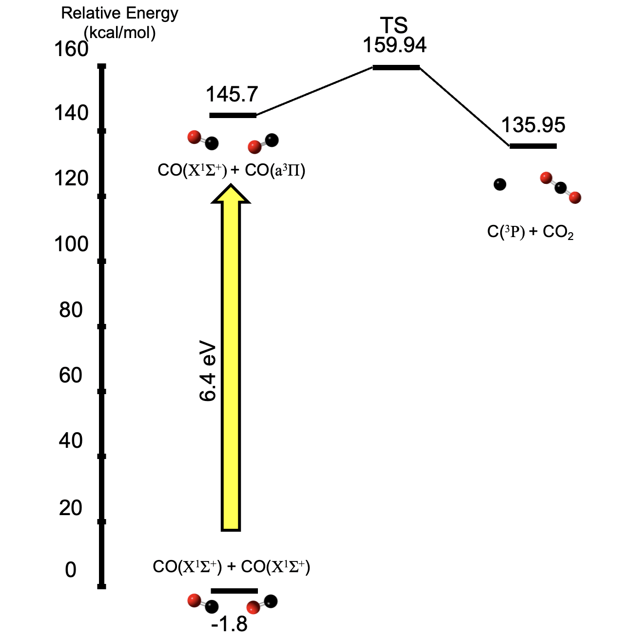

II.6 Model simulation and analysis
With the reaction mechanism built following the procedure mentioned above, simulations (solving differential equations) were performed for the reaction time of 18 hours (i.e. 64800 seconds) on eight experimental conditions of Fleury et al. 2019 (i.e. With UV and without UV at each T = 573, 873, 1173, and 1473 K with the initial composition of 99.7 % of and 0.3% of CO) and four experimental conditions of Fleury et al. 2020 (i.e. With UV and without UV at each T= 1173 and 1473 K with the initial composition of 99.26 % of , 0.26% of CO, and 0.48 % of ) using reaction mechanism simulator (RMS, Johnson et al. 2019), a package included in the RMG (Gao et al. 2016) suite package. The model output is a set of temperature-dependent molecular mixing ratio profiles of each of the species, summarized in Figures 6, 8a, and 9, which add up to 1 (e.g. a molecular mixing ratio of 10-6 in Figure 6 refers to 1 ppm).
Additional model simulations were performed on the same experimental conditions of Fleury et al. 2019 except for higher temperatures (i.e. each T = 2000 and 2500 K). The model simulation for longer reaction time (206 hours), higher pressure (81 mbar), and the temperature of 1473 K was also performed using RMS. The reactor was assumed as isobaric, isothermal, and homogeneous. Rate of production analysis (ROP) was done using the RMS and the ROP analysis of the kinetic model describing Fleury et al. 2019 is available in the Appendix A. Sensitivity analysis was done using the RMG suite package (Gao et al. 2016).
III Results and Discussions
III.1 + CO(a3) reaction rate coefficients
As it is shown in Table 2 and Figure 3, the rate-coefficient of the + CO(a3) H + HCO reaction is at least 10 orders of magnitude faster than the rate coefficients of any other channels, which indicates that the reaction between UV-excited CO and will dominantly proceed into H and HCO molecules at any temperature and pressure conditions. The + CO(a3) H + HCO reaction is also called as a ”well-skipping reaction” which refers to an elementary reaction that traverses more than one transition-state dividing surface in a single elementary step (see Figure 2). This well-skipping behavior is mainly attributed to UV-excited CO’s excessively high potential energy compared to the potential energy of all the other species and transition states. As shown in Figure 2, the potential energy of (photo)chemically activated reactants (i.e. + CO(a3)) is already 40 kcal/mol above the second highest potential energy (i.e. the potential energy of TS4, 104.9 kcal/mol). For this reason, even at higher pressure condition of 100 bar, increased collisional stabilization into other stable molecules (i.e. HCOH isomers and ) is still not efficient enough to beat this well-skipping reaction to form HCO and H. For a similar reason (i.e. excessive energy from UV-photons), the UV-excited well-skipping channel is less sensitive to temperature changes compared to other reaction channels. However, this is not the case when CO is in the ground state. As can be seen from Table 2, in the case of the reaction between and CO in the ground state (i.e. X1), the reaction channel of + CO(X1) stays as a main channel up until 1173 K, while the well-skipping reaction (i.e. + CO(X1) H + HCO) takes over the main channel from the + CO(X1) channel at 1473 K (see numbers in parentheses in Table 2). This is because the only energy source for the reactants ( + CO(X1) to overcome the reaction barrier of 103.4 kcal/mol (i.e. TS5 in Figure 2) to form HCO and H is from thermal energy. Up until 873 K, thermal energy is not enough so the intermediates that overcome the reaction barrier of 81.8 kcal/mol (i.e. TS1) will stabilize into rather than skipping all the other wells to form HCO and H. With increasing temperatures above 1173 K, the reactants are more thermally energized so that they are more likely to proceed to the well-skipping channel (i.e. + CO(X1) H + HCO) and competing with the stabilization channel down to . So the major difference between the + CO chemistry with and without UV photons would be whether this well-skipping channel (i.e. + CO H + HCO) is dominant (i.e. with UV) or not (i.e. thermal-only). These results demonstrate the importance of rigorous reaction kinetics modeling, including photochemical reaction pathways. In the previous study by Fleury et al. 2019, the CO(X1) + CO(a3) C(3P) + reaction was considered as the only important photochemistry regardless of dominant in the system. It was not immediately evident that the reaction + CO(a3) H + HCO reaction is the most predominant channel and has several orders of magnitude higher rate coefficients than other reaction channels (e.g. + CO(a3) ). This has the important consequence that the H atoms generated are now very reactive and start radical chain reactions.
III.2 CO(X1) + CO(a3) C(3P) + reaction reaction rate coefficients
As it is shown in Figure 4, the CO(X1) + CO(a3) reaction has a non-zero reaction barrier (i.e. 14.24 kcal/mol) even after the photoexcitation of the ground state CO, different from + CO(a3) reactions (i.e. barrier-less reactions). For this reason, the calculated reaction rate coefficient shows significant positive temperature dependency as shown in Figure 4. The last row of the Table 2 shows 4 orders of magnitude difference between the rate coefficient at the lowest temperature (i.e. 573 K) and the rate coefficient at the highest temperature (i.e. 1473 K). So we can easily predict that this reaction will play a more significant role at elevated temperatures. It is also clear from the Table 2 that this reaction would be insignificant without UV photons (even at 1473 K, the rate-coefficient is still smaller than 10-13 cm3/mol/s), which makes a major difference between the chemistry with and without UV photons (i.e. thermal-only).
III.3 Modeling of the /CO exoplanet atmosphere analogue of Fleury et al. 2019
III.3.1 Reaction kinetics of thermal-only chemistry
As shown in Figure 6, all major species (i.e. , , , and H radical) formations under thermal-only conditions are predicted to be extremely temperature dependent. This is mainly attributed to elevated reaction rate-coefficients with increasing temperature, leading to the formation of major species. This predicted behavior qualitatively matches well with the previous experimental results of Fleury et al. 2019 using the quartz cell. For example, the absorption infrared (IR) spectrum of and show up at 573 K and increase with temperatures. The model predicts that the molecular mixing ratio of these molecules might be too low ( 10-28 or lower) to be observed experimentally, but it has to be noted that the surface chemistry happening on the wall of the quartz cell might have affected the reaction chemistry. Compared to and , has much lower absorption cross-sections of IR, thus the IR peaks of start showing up at 1173 K in the quartz cell used in Fleury et al. 2019. The predicted molecular mixing ratio of and after the reaction time of 18 hours are almost same. This predicted behavior is due to their formation pathways shown in Figure 7a. According to the ROP analysis (see Appendix A), the predicted major precursors of and all over the reaction time (i.e. 18 hours) are and OH, respectively. These radical species (i.e. and OH) are simultaneously formed through the reaction HCOH + + OH at all temperature conditions (additionally formed through the reaction + H + OH at the temperatures above 1173 K), and respectively react with to form their corresponding stable species along with the H atom. Up until 1173 K, HCOH is directly formed through the reaction + CO HCOH followed by HCOH + + OH or the unimolecular reaction (i.e. isomerization) into . However, at temperatures above 1173 K, starts to isomerize back to HCOH, which eventually leads to increased formation of and . can also be formed through either + CO at all temperature conditions or HCO + + H (only at T 873 K). HCO forms through + CO H + HCO, but readily dissociates back to CO + H. However, as mentioned previously, at T 873, HCO can proceed to by reacting with and at T 1473 K, HCO can be produced through the additional reaction H + CO HCO.
H radicals are formed in a significant amount at T 873 K through thermal dissociation into H radicals (i.e. 2H), while the recombination back to (i.e. H + H ) becomes significant at T 1473 K after H radicals being formed enough in the system. is formed through CO + OH H + at T 1173 K. But at T 1473 K, is formed through + CO + , while reacts with H radical and forms CO and OH (not indicated in Figure 7a). This reaction (i.e. + H CO + OH) is attributed to an increased amount of H radicals due to elevated thermal dissociation of at elevated temperatures. Overall, as can be seen from Figure 7a, with increasing temperatures, additional reaction pathways are being added to the system and push the chemistry to the right side of the figure toward the formation of , and .
It is also interesting to observe that the model predictions of molecular mixing ratios of species at thermal-only conditions becomes similar to those at the condition with UV photons at around 2000 K. At T = 1970 K, the amount of , , and formed in the system with UV photons was only different by less than 10 % compared to that in the thermal-only system. In this paper, we will call this temperature a ”transition temperature” with regard to these species (i.e. , , and ). This indicates that at temperatures higher than 2000 K, thermally driven reactions are fast enough so that the system becomes less sensitive to UV photons compared to the system at lower temperatures. This feature has already been suggested from previous theoretical studies (Moses et al. 2011; Venot et al. 2012; Moses 2014). However, it has to be noted that there are multiple factors (e.g. other photochemical reactions not considered in this study, temperature-dependent UV-photoabsorption cross-sections of carbon monoxide, etc.) that can change the transition temperature and this will be discussed later. Also, it is predicted from the model that the molecular mixing ratios of all major species (i.e. , , and ) decrease at the temperature above this transition temperature, which means that all these major species have reached quasi-equilibrium and are not favored at this temperature condition anymore. In case of , the decrease in molecular mixing ratio at temperatures higher than 2000 K is more significant compared to molecular mixing ratios of and . This behavior is due to the thermal conversion of into species (mainly ). This will be discussed in detail in a later section.

(a) (b)
III.3.2 Reaction kinetics of thermal- and UV-photochemistry
The most notable feature shown from the reaction kinetic modeling of simultaneous thermal- and UV-photochemistry is the significant increase of the molecular mixing ratios of all the species at all temperatures compared to the case with thermal-only chemistry (see Figure 6). All the species (i.e. , , , and H radicals) are predicted to be produced at least 20 orders of magnitude, 7 orders of magnitude, and 3 orders of magnitude more in the thermal- and UV-photochemistry condition than in the thermal-only condition at temperatures of 573 K, 873 K, and 1173 K, respectively. At temperature of 1473 K, all these species are predicted to be formed 40 times more in the thermal- and UV-photochemistry condition compared to the predicted productions of the species in the thermal-only condition. Figure 6b shows that the molecular mixing ratio of CO(a3) is not sensitive to temperature difference, which indicates that only the photochemical cycle (mentioned later) determines its abundance in the system. Overall, the model prediction can well explain significantly augmented formations of , , and at all temperature conditions (T 1473 K) under simultaneous thermal- and UV-photochemistry, as shown in Figure 6 of Fleury et al. 2019.
If we look at the major reaction pathways based on the ROP analysis as shown in Figure 7b, we can see that the chemistry of the whole system at all temperature conditions is dominated by one photochemical cycle indicated in the yellow highlighted region: (i) Carbon monoxide in the ground state gets electronically excited to the a3 state by UV-photons, (ii) Excited CO can either go down to the ground state CO within its radiative lifetime of 3 ms (Lee et al. 2020) or react with to form H and HCO, and (iii) HCO can either dissociate into H + CO or react with H radical to disproportionate to and CO. At elevated temperatures, H radical recombination (i.e. H + H at T 873 K) and dissociation ( H + H at T 1473 K) also become dominant as well. Based on the ROP analysis, these major reaction pathways of the highlighted cycle are at least 3 orders of magnitude faster than any other reactions shown (or not shown if they are minor reactions) in Figure 7b. For this reason, a significant amount of HCO becomes available with the aid of this photochemical cycle even at very low temperature such as 573 K, which makes the chemistry of the system very different from thermal-only chemistry. As a result, every chemical reaction that is involved with HCO becomes much more efficient with UV-photons than it used to be in thermal-only chemistry, which in turn pushes the whole chemistry to the right side of the Figure 7b and eventually leads to the augmented formation of , , and , in agreement with the experimental observations of Fleury et al. 2019.
The reaction between the photoexcited CO and the ground-state CO that forms a triplet C atom and turns out to be very important according to the kinetic model especially at high temperatures above 873 K. As shown in Figure 7b, this reaction efficiently forms and the triplet C atom first. The C atom will then be hydrogenated by reacting with into CH, , and then step by step, which will form . Along with every hydrogenation step (i.e. CHn + CHn+1 + H), H radicals are efficiently formed and then attack to form OH radicals as well, which will form . As mentioned earlier in the section III.2, due to its temperature-dependency of the CO(X1) + CO(a3) C(3P) + reaction, this reaction will be more important at elevated temperatures. According to our kinetic model result, significantly augmented formations of major species (, , and ) are attributed to the + CO(a3) H + HCO reaction up until 873 K, while the augmented major species formations are attributed to the CO(X1) + CO(a3) C(3P) + reaction at temperatures above 873 K. In short, two different photochemical schemes (i.e. + CO(a3) H + HCO vs CO(X1) + CO(a3) C(3P) + ) determines the mixing ratios of , , and at different temperature regions below the transition temperature (i.e. 1970 K for , , and ), respectively. With regard to H radicals, however, it has to be noted that + CO(a3) mainly determines the mixing ratio of H radicals in the system at temperatures below the transition temperature (i.e. 1650 K for H radicals).
In contrast to thermal-only chemistry, the molecular mixing ratio of , , and wiggles as shown in Figure 6a. These molecules have been efficiently formed as a result of UV photochemistry enhanced by metastable a3 state carbon monoxide and remain relatively stable at relatively lower temperatures below 873 K (i.e. UV photochemistry determines their mixing ratio after the reaction time of 18 hours). However, at 1173 K, thermal chemistry starts to partially determine their mixing ratio and this is well-shown at 2000 K in Figure 6a where the molecular mixing ratios of , , and formed with UV photons are not distinguishable from those formed without UV photons (i.e. thermal only). We further simulated the molecular mixing ratio of , , and at 2000 and 2500 K after 18 hours while maintaining other conditions as same as that at 1473 K, and as expected, there was no significant difference in the molecular mixing ratio of , , and formed no matter whether UV photons were available or not (see Figure 6). So based on the model prediction (and as mentioned earlier in the text), we can say that the transition temperature where thermal chemistry becomes dominant compared to photochemistry starts at around 1970 K and it has to be noted that this transition temperature can be shifted due to multiple factors including (i) errors in the UV photon fluxes, (ii) errors in photoabsorption cross-sections (e.g. temperature dependent) of species, (iii) errors in quantum yields of any photochemical reactions, (iv) any missing reaction species or reactions in the system, (v) any errors in included thermal reactions, and (vi) any errors in included thermodynamic parameters of related species. With regard to this, the sensitivity of the model will be discussed later.
III.3.3 The potential importance of the acetylene () formation with regard to the organic refractory aerosol formation in hot-Jupiter exoplanet atmospheres
Although a detectable amount of solid-phase product was not observed from any of the experiments at the temperature below 1473 K conducted by Fleury et al. 2019 (i.e. 15 mbar; 573–1473 K; with and without UV; reaction time of 18 hours), an observable amount of condensed-phase organic aerosol products as a thin film deposited on sapphire windows was reported by Fleury et al. 2019 after 204 hours of experiments with increased starting total gas pressure of 81 mbar with UV irradiation at 1473 K. Since there was no any direct information about the molecular structure of this aerosol, it is hard to exclusively say whether this observed organic aerosol is composed of aromatic hydrocarbons (if not polycyclic) or not. However, it is logical to say that species should first go through species before growing into aerosol particles, which gives us a rationale to look into any or larger species predicted to be formed during our model simulation. The model simulation of the corresponding experimental condition (i.e. 81 mbar, 1473 K, with UV-photons, and the reaction time of 206 hours) predicted the molecular mixing ratio of each species as following: [] = 6.6210-15, [] = 7.3210-12, and [] = 1.9510-10. Any species larger than species (e.g. or larger) were predicted to be around or less than 1.0010-20 (the absolute tolerance of the differential equation solver), which indicates that no significant amount of the species larger than species are predicted to be formed in the simulated systems even at the temperature of 2500 K.
Among these species, we focused on the acetylene formation in the model for the following reason: (i) Previous studies have suggested benzene (1-ring aromatic hydrocarbon) and naphthalene (2-ring aromatic hydrocarbon) as precursors to refractory hydrocarbon aerosols (Trainer et al. 2013; Brem et al. 2015), (ii) one of the prevailing mechanisms that rationalize the formation up to 2-ringed aromatics (including benzene and naphthalene) is the hydrogen-abstraction-acetylene-addition mechanism (HACA), an aromatic radical formed via hydrogen abstraction adds to acetylene () to form a larger vinylic radical adduct (Bittner & Howard 1981; Chu et al. 2019; Frenklach et al. 1985; Parker et al. 2014; Yang et al. 2016; Smith et al. 2020), and (iii) a previous photochemical experiment by Franklin 2018 using a -lamp (115–170 nm) at 25∘C in oxygen-free conditions has shown that the VUV irradiation on is the most efficient in the formation of organic particles compared to the VUV irradiation on other species (i.e. and ). Although it is not clear how the acetylene formation is exactly related to the formation of organic aerosols observed from Fleury et al. 2019, as mentioned earlier, many previous studies indicate the positive relationship between the acetylene formation and the aerosol formation.

| 1473 K, 15 mbar b | 1473 K, 81 mbar | 1473 K, 81 mbar b,c | 2000 K, 15 mbar | 2500 K, 15 mbar | |
|---|---|---|---|---|---|
| (18 hr) | (18 hr) | (206 hr) | (18 hr) | (18 hr) | |
| [] | 1.1010-11 (2.6810-14) | 1.5710-12 (2.1810-13) | 1.9510-10 (2.4310-11) | 1.3710-7 (1.2510-7) | 8.5510-8 (8.5510-8) |
Note. — aNumbers in parentheses refer to calculated molecular mixing ratio of at thermal-only condition; bExperimental conditions conducted by Fleury et al. 2019; cExperimental condition from which a detectable amount of solid-phase product was observed in Fleury et al. 2019
With this background, if we look at the temperature-dependent mixing ratio profiles of acetylene predicted by the reaction kinetic modeling for the experimental conditions described in Fleury et al. 2019, we can see that UV-excited metastable carbon monoxides can significantly enhance the formation of acetylene compared to thermal-only chemistry as shown in Figure 8a at the temperature up to 1473 K. Up until 1173 K, acetylene () is predicted to be produced at least 4 orders of magnitude more in the thermal- and UV-photochemistry condition than in the thermal-only condition as shown in Figure 8a. At the temperature of 1473 K, acetylene is predicted to be formed 410 times more in the thermal- and UV-photochemistry condition compared to the predicted acetylene production in the thermal-only condition. At the temperature above 2000 K, there was no significant difference in the predicted molecular mixing ratio of formed no matter whether UV photons were available or not, which indicates that the transition temperature is around 2000 K (precisely 1985 K). Figure 8b shows major reaction pathways from species to . As can be seen from Figure A10–A13 in the Appendix A, at early timescales (i.e. up to 10 ms), + CO + OH is the major pathway, and then the major formation pathway changes to others such as HCCOH + H + OH or + H + OH. With UV photons available in the system, the UV-elevated amount of HCO results in the elevated formation of HCOH and , which then results in the elevated formation of . However, at temperatures higher than the transition temperature (i.e. 1985 K), thermal chemistry now determines the mixing ratio like it did with the molecular mixing ratios of , , and . Like the calculated rate-coefficient of the reaction between the excited CO and forming HCO and H is much faster than the rate-coefficient of the reaction between the ground state CO and forming HCO and H, the rate-coefficient of the reaction between the excited CO and forming and OH might affect the formation of in a significant way. To test this, we recalculated the potential energy surfaces of + OH taken from Miller & Melius 1989 at the CBS-QB3 level of theory using Gaussian 09 (Frisch et al. 2009) and calculated the temperature- and pressure-dependent rate coefficients of + CO(a3) reactions following the similar method described in II.4 (rate-coefficients and the corresponding PES are available in the Supplementary Materials). However, no matter whether + CO(a3) chemistry is included in the reaction kinetic model or not, no significant change was observed on the formation of . This might indicate that the molecular mixing ratio of is still too low to draw any significant increases in the acetylene formation through + CO(a3) chemistry.
Table 3 shows the model (thermal- and UV-photochemistry incorporated) predicted mixing ratios at different conditions (starting from : CO = 99.7 : 0.3). You can see from the Table 3 that the model simulation indicates that the formation of acetylene () is favored with increasing temperature. The model also shows that formation has not reached quasi-equilibrium state even after 206 hrs (81 mbar) and 18 hrs (15 mbar) at 1473 K, respectively (see Figure B14a–b in the Appendix B). However, at 2000 K, the acetylene formation reaches its quasi-equilibrium state after 18 hrs with its molecular mixing ratio of 1.3710-7 (see Figure B14c in the Appendix B) and no significant amount of any species larger than molecules were predicted in the given system. This mainly indicates that (i) the amount of acetylene formed via thermal-only chemistry (up to 2500 K) from the condition of : CO = 99.7 : 0.3 is not enough to push the chemistry to larger species such as polycyclic aromatic hydrocarbons (PAHs) that are accepted as precursors to organic aerosols in the majority of combustion research (Frenklach & Mebel 2020) and (ii) some major photochemical reactions can bring the chemistry into disequilibrium chemistry to form larger hydrocarbon species (e.g. 1-ring aromatic hydrocarbons or PAHs) or even organic aerosols. With regard to (ii), the results of previous experimental studies (Franklin 2018 and Fleury et al. 2019) in combination with the current study in this paper might indicate that the reaction kinetic model including the -photochemistry is the key to explain the experimentally observed organic aerosol formations from Fleury et al. 2019. Note that our reaction kinetic model including CO(a3)-photochemistry was successful in qualitatively explaining the significant augmented formation of major species (i.e. , , and ) observed in Fleury et al. 2019 at all temperature conditions. As can be seen from Table 3, our thermal- and UV-photochemistry model predicts 3 orders of magnitude more are formed in the system at the 2000 K and 15 mbar condition even with an order of magnitude shorter time scale (i.e. 18 hrs) compared to the 1473 K and 81 mbar condition with the reaction time of 206 hrs. Thus if our hypothesis (i.e. the amount of is closely related to aerosol formations) is correct, we are able to observe aerosol formations even at temperatures lower than 2000 K within the reaction time shorter than 18 hrs from the same experimental device of Fleury et al. 2019. Conducting this experiment and including -related photochemistry into our current model would be interesting future studies.
III.3.4 Sensitivity analysis of the kinetic model
One of the major features of this study is the assessment of the transition temperature in which thermal chemistry starts to become dominant compared to photochemistry. However, this transition temperature can be affected by multiple factors as mentioned earlier: (i) errors in the UV light sources, (ii) errors in photoabsorption cross-sections, (iii) errors in quantum yields of any photochemical reactions, (iv) any missing reaction species or reactions (even surface chemistry), (v) any errors in thermochemical reactions included in the model, and (vi) any errors in thermodynamic parameters of related species. Although (iv) is important when it comes to model improvements, this was beyond the scope of the current work. With regard to (i)–(iii), these three factors directly affect the calculated carbon monoxide photoexcitation rate-coefficient (i.e. X1 a3) in II.3. With regard to (v)–(vi), these errors originally came from the embedded errors of rate coefficients imported from the references described in II.1. We computed the sensitivity of the major species (i.e. , , and ) to all of the rate coefficients in the model simulated under the condition of 1473 K, 15 mbar, [] = 0.997, and [CO] = 0.003, and the most sensitive three parameters that affect the predicted formation of the major species turn out to be photochemical reactions which are
| (2) |
| (3) |
| (4) |
They each have normalized sensitivities with magnitudes of around 1, 0.95, and -0.75, respectively (see Figure C14). This means that, for example, if one increases the rate-coefficient of reaction 2 by a factor of 10, the predicted molecular mixing ratio of the major species (i.e. , , and ) would be increased by 10 times and the transition temperature would be pushed to a much higher temperature. On the contrary, if one reduces this carbon monoxide photoexcitation rate-coefficient (i.e. reaction 2, k2) by a factor of 2, the predicted molecular mixing ratio of the major species (i.e. , , and ) would be decreased by 50% and the transition temperature would be shifted to lower temperature. The former case is possible if the photoabsorption cross-sections of carbon monoxide are underestimated. It has to be noted that the photoabsorption cross-sections of CO used to calculate k2 were taken from Myer & Samson 1970 which experimentally measured the VUV absorption cross-sections at 298 K. Since VUV absorption cross-sections usually increase with increasing temperatures due to thermally increased populations at higher vibrational states, which then might result in increased access to upper electronic states. Venot et al. 2018 experimentally showed that the photoabsorption cross-sections of around Lyman- can vary by two orders of magnitude between 150 and 800 K. For this reason, it might be the case if the photoabsorption cross-sections of CO around Lyman- increase by more than an order of magnitude from 298 K to 1473 K, which can potentially increase the carbon monoxide photoexcitation rate-coefficient (i.e. k2) by a factor of 10, which means the calculated k2 is 10 times underestimated. However, the latter case (i.e. reducing k2 by a factor of 2) is also possible. It has to be noted that the quantum yield (i.e. ) used in the calculation of k2 in II.3 is assumed to be unity since we couldn’t find any theoretically or experimentally determined quantum yield of this photoexcitation reaction. However, it wouldn’t be surprising if is 0.5. In this case, the model predicted molecular mixing ratio would be overestimated by 50%. These cases suggest interesting future studies (i.e. a measurement of temperature-dependent VUV photoabsorption cross-sections of carbon monoxide or a determination of the ).
It has to be noted that there are too many model parameters and too few experimental data (e.g. a measurement of the CO absorption cross-section at various temperatures or a measurement of ) to allow a perfect determination of the model parameters (and keep in mind that there are several other moderately sensitive rate coefficients and thermochemistry in the model, not just these 3 most sensitive reactions). However, even considering these, our kinetic modeling work indicates that electronically excited CO in its metastable state (a3) can push the whole chemistry to the augmented formation of , , and in an obvious way, which qualitatively matches well with the experimental observation from Fleury et al. 2019. The quantitative discrepancy doesn’t indicate a fundamental issue with the reaction kinetic model, but rather reflects our imperfect knowledge of the values of the model parameters.
III.4 Modeling of the /CO/ exoplanet atmosphere analogue of Fleury et al. 2020
When is added to the /CO mix to change the C/O ratio to more realistic solar elemental abundance, both of the kinetic model-predicted thermal-only and UV-incorporated thermal chemistry of Fleury et al. 2020 were almost similar to those of Fleury et al. 2019. The major reaction pathway forming (note that was included from the beginning of the experiments at much higher mixing ratio, so not focused as a product) in Fleury et al. 2020 are predicted to be almost similar to those described in Figure 7 and the previous section of describing the modeling result of Fleury et al. 2019. The major reaction pathways forming was exclusively CO being oxidized by OH radicals forming and H radicals. This behavior is due to a huge amount of included in the system from the beginning, which then can either thermally or photochemically dissociate into H and OH radicals in the system. Although the formation is predicted from our model simulation of Fleury et al. 2019, the amount of the predicted in the simulation of Fleury et al. 2019 is still way smaller than the amount of introduced into the system from the beginning of the simulation of Fleury et al. 2020. For this reason, the simulated system of Fleury et al. 2020 would contain much more OH radicals compared to the simulated system of Fleury et al. 2019. This leads to the notable difference between the model simulation of Fleury et al. 2020 and that of Fleury et al. 2019 in the form of the reversed molecular mixing ratio of to . As shown in Figure 9, the molecular mixing ratio of is 3 orders and 4 orders of magnitude larger compared to that of at 1173 and 1473 K, respectively. In the case of Fleury et al. 2019, the molecular mixing ratio of is always at least 2 orders of magnitude higher than that of at temperatures higher than 1173 K, no matter UV photons are available or not. As mentioned above, this reversed ratio is attributed to the inclusion of from the beginning of the kinetic simulation of Fleury et al. 2020. According to the kinetic modeling, already thermally dissociates to form both H and OH radicals at 1173 K. These OH radicals reach the quasi-equilibrium state within 11 hours when the energy source is thermal-only, while they reach quasi-equilibrium much faster within 200 seconds with the aid of UV photons (i.e. photodissociation of into H + OH). This tendency gets more severe at higher temperature (i.e. 1473 K) in which thermal dissociation becomes much more efficient (since the thermal dissociation rate-coefficient is positively temperature dependent). This can be observed in the form of increasing OH mixing ratio in Figure 9. Compared to 1173 K, the experimental condition of Fleury et al. 2020 is much more oxidizing, so that the predicted mixing ratio decreases rapidly by 20 times (i.e. from [] = 1.9710-8 at 1173 K to [] = 9.5510-10 at 1473 K). It also has to be noted that the mixing ratio doesn’t show any difference whether UV irradiation is available or not (see red symbols and lines in Figure 9). This feature indicates that the formation has already reached its thermal quasi-equilibrium after 18 hours. If you look at Figure D17 in Appendix D, mixing ratio at 1173 K reaches equilibrium within 7 hours in thermal-only condition, and 50 seconds with UV-irradiation, while mixing ratio at 1473 K reaches equilibrium within 200 seconds in thermal-only condition, and 30 seconds with UV-irradiation. According to our model prediction, the predicted methane molecular mixing ratio at 1173 K is enough to be detected (i.e. [] = 1.9710-8 which is around the same to the predicted mixing ratio of plotted on Figure 6a at 1173 K with UV irradiation). However, it was surprising that no methane formation was observed in any of experiments in Fleury et al. 2020. Two plausible explanations can be (i) errors in the current model overestimated the amount of formation or (ii) significant amount of included in the system from the beginning has disturbed the detection of any IR or mass-spectrometry peaks of at 1173 K. With regard to (i), we can simply assess this by sensitivity analysis. According to sensitivity analysis, the most sensitive reaction and the most sensitive thermochemistry that affect the predicted formation of are the reaction + OH + H and the thermochemistery of with their normalized sensitivities of 0.5 and 1.25, respectively (see Figure C16c and d in Appendix C). This means that we have to reduce the rate-coefficient of reaction 2 by 20 times or we have to reduce the Gibbs free energy of by 72 % in order to decrease the predicted mixing ratio of by 5 times. Although it is obvious that those parameters embed a certain amount of errors inside, it is less likely that these errors can solely explain the non-detection of in Fleury et al. 2020. Rather, it would be more reasonable to lean to the explanation (ii) (i.e. an interference on the IR peaks and mass-spec peaks of due to significant amount of pre-existing in their experimental condition of Fleury et al. 2020). Other than that, the current model’s reaction kinetic interpretation qualitatively matches well with the experimental observation of Fleury et al. 2020.

III.5 Quantitative comparison on the mixing ratio of between the model simulation results and the experimental results of Fleury et al. 2019 and Fleury et al. 2020
Since Fleury et al. 2019; Fleury et al. 2020 quantified the mixing ratios of at various experimental conditions using the Beer-Lambert law on the IR spectroscopy results, we tried to derive some quantitative comparisons of between the model simulation results and the experimental results at corresponding experimental conditions. Although the discrepancy between the model simulation results and the experimental results of the C/O=0.35 condition is within 2 orders of magnitude as it is shown in Table 4, the discrepancy between the model simulation results and the experimental results of the C/O=1 condition is way larger compared to the discrepancy in the C/O=0.35 condition. There are multiple factors that can derive this discrepancy. First, as mentioned in the main text, the products that are observed in gas-phase static cell experiments conducted by Fleury et al. 2019; Fleury et al. 2020 are formed far beyond tertiary or even further reaction chemistry including surface chemistry on the wall since these experiments were conducted for more than 18 hrs. Surface chemistry is considered to be more efficient and faster compared to gas-phase chemistry and very difficult to simulate in detail. Although surface chemistry is indeed very important when it comes to precisely describe experimental study, it was beyond the scope of the current work to gain a better insight into simultaneous thermally and photochemically driven reaction pathways involving electronically excited CO in its metastable state (a3). Natural isotopic contamination when using enriched isotopic gases was mentioned in Fleury et al. 2019 and affected the chemistry that might have led to the discrepancy as well. The calculation of the absorption cross-section of described in the section 2.5 in Fleury et al. 2019 can also affect the discrepancy as well. We conclude it is likely that discrepancy is mainly due to combined effects of these multiple factors mentioned above as well as experimental uncertainties. As mentioned earlier, the quantitative discrepancy doesn’t indicate a fundamental issue with the reaction kinetic model, but rather reflects our imperfect knowledge of the values of the model parameters.
Keeping the quantitative comparison aside that can be influenced by the experimental conditions discussed above, our modeling work clearly predicts the experimental observations: (a) for C/O=1, where only and CO molecules were present in the beginning, the thermochemical formation of is significantly less efficient than thermally augmented photochemical production of , as observed by Fleury et al. 2019; (b) for C/O=0.35, which was achieved through the addition of to the + CO starting composition, chemistry is mainly driven by the dissociation (both thermally and photochemically) and no significant difference is observed between thermal and thermally augmented photochemical reaction pathways as a result. Our model again confirms the experimental observations of Fleury et al. 2020.
This analysis also highlights the importance of both experimental work and rigorous theoretical reaction kinetics modeling. Further, this work confirms that though experimental conditions have limitations that are unavoidable (such as reaction cell boundaries), relative equilibrium mixing ratios obtained from the experiments are similar to the predicted ones.
| C/O=1 | C/O=0.35 | |||||||
|---|---|---|---|---|---|---|---|---|
| Thermal only | Thermal + UV | Thermal only | Thermal + UV | |||||
| This study | Exp. 2019a | This study | Exp. 2019b | This study | Exp. 2020c | This study | Exp. 2020c | |
| 573 K | 1.8310-31 | 1.5010-5 | 7.6010-10 | 1.0010-3 | N/A | |||
| 873 K | 4.9610-17 | 6.4010-5 | 4.5610-10 | 8.5010-4 | N/A | |||
| 1173 K | 6.8810-14 | 3.8010-5 | 5.3310-11 | 1.2010-3 | 1.0810-5 | 3.5010-4 | 1.0810-5 | 8.8010-4 |
| 1473 K | 1.6810-12 | 3.4010-5 | 7.2110-11 | 4.3010-4 | 5.5610-6 | 3.6010-4 | 5.5610-6 | 5.6010-4 |
Note. — aMixing ratios of 13 taken from Table 2 in Fleury et al. 2019; bMixing ratios of 13 taken from Table 3 in Fleury et al. 2019; cMixing ratios of 13 taken from Table 3 in Fleury et al. 2020
III.6 Impact of the current study on the field of astrochemistry
In this work, we have implemented the state-of-the-art computer-aided automatic construction of an astrochemical reaction network and successfully demonstrated how this computer-aided reaction kinetic model can help us precisely interpret the previous photochemical experiment in detail. Not only we have figured out the photochemically important role of the UV-excited state of carbon monoxide, but also we suggest future studies such as the measurement of temperature-dependency of the cross-sections of carbon monoxide or the experiment and modeling combined kinetic study of -UV-photochemistry. Our work clearly demonstrates the importance of coupling photochemical reaction pathways to thermochemical models to better understand exoplanet atmospheres. Only then will we be able to realistically describe atmospheric chemistry of exoplanets that receive significant amount of UV photons from their parent stars. The JWST transmission spectroscopy data will keep providing us with the deluge of exoplanetary data that need to be efficiently and precisely interpreted by atmospheric chemical models. As we can see from the case of the recent study by Tsai et al. 2022, it is important to properly implement photochemical reactions in chemical models to properly interpret observational data and extract valuable insight on exoplanet atmospheres. We hope our study would be the benchmark for future exoplanet atmospheric photochemical modeling study that will consequently lead to a rapid innovation in the field of astrochemistry.
IV Conclusions
In this work, we utilized an automatic chemical reaction mechanism generator to build a large and complex thermo- and photochemical network that can qualitatively rationalize the augmented chemistry observed from previous experimental works by Fleury et al. 2019; Fleury et al. 2020. Our model has demonstrated that Lyman--aided electronically excited carbon monoxide in its metastable state (a3) can significantly enhance the chemistry in the exoplanet atmosphere-like conditions through two different reactions which are (i) + CO(a3) H + HCO and (ii) CO(X1) + CO(a3) + C(3P). The first reaction (i.e. + CO(a3) H + HCO) leads to significantly augmented formation of HCO radicals in -dominated system, which can push the whole chemistry to further , , and formation even at a very low temperature of 573 K. At temperatures above 873 K, the second reaction (i.e. CO(X1) + CO(a3) + C(3P)) forms and the triplet C radicals which rapidly hydrogenate into , which mainly contributes to significantly augmented formation of major species. However, at temperatures above 2000 K, thermal chemistry then becomes efficient enough to dominate the whole chemistry. Given the experimental conditions of Fleury et al. 2019; Fleury et al. 2020, the transition temperature in which thermal chemistry becomes dominant compared to photochemistry starts at 1970 K, and this transition temperature can be shifted due to multiple factors. Finally, under the experimental conditions of Fleury et al. 2019; Fleury et al. 2020, our model might suggest that thermal-only chemistry up to 2500 K cannot push the chemistry to larger species such as PAHs or even organic aerosols, and instead, photochemistry and the photochemistry of higher carbon species that are produced from photochemistry might be the key to explain the experimentally observed hydrocarbon aerosol formations observed from the previous experiments by Fleury et al. 2019. The model results have demonstrated the importance of electronically excited metastable carbon monoxide in exoplanet atmospheres and that adding more photochemical reactions and species to current 1D photochemical models would provide a more comprehensive understanding of exoplanet atmospheres.
This research work was carried out at the Jet Propulsion Laboratory, California Institute of Technology, under a contract with the National Aeronautics and Space Administration. This research work was funded by the NASA Exoplanet Research Program grant to MSG. BF thanks the Université Paris-Est Créteil (UPEC) for funding support (postdoctoral grant).
References
- Allen et al. (2012) Allen, J. W., Goldsmith, C. F., Green, W. H., & West, R. H. 2012, Phys. Chem. Chem. Phys., 14, 1131, doi: 10.1039/C1CP22765C
- Backx & Van der Wiel (1976) Backx, C. Wight, G. R., & Van der Wiel, M. J. 1976, J. Phys. B: Atom. Mol. Phys., 9, 315, doi: 10.1088/0022-3700/9/2/018
- Bittner & Howard (1981) Bittner, J. D., & Howard, J. B. 1981, Symp. Combust. Proc., 18, 1105–1116, doi: https://doi.org/10.1016/S0082-0784(81)80115-4
- Brem et al. (2015) Brem, B. T., Durdina, L., Siegerist, F., et al. 2015, Environ. Sci. Technol., 49, 13149–13157, doi: https://doi.org/10.1021/acs.est.5b04167
- Chu et al. (2019) Chu, T.-C., Buras, Z. J., Smith, M. C., Uwagwu, A. B., & Green, W. H. 2019, Phys. Chem. Chem. Phys., 21, 22248–22258, doi: https://doi.org/10.1039/c9cp04554f
- DeVine et al. (2022) DeVine, J. A., Choudhury, A., Lau, J. A., Schwarzer, D., & Wodtke, A. M. 2022, J. Phys. Chem. A, 126, 2270, doi: https://doi.org/10.1021/acs.jpca.2c01168
- Drummond et al. (2019) Drummond, B., Carter, A. L., Hebrard, E., et al. 2019, MNRAS, 486, 1123–1137, doi: https://doi.org/10.1093/mnras/stz909
- Euclides & Barreto (2019) Euclides, H. O., & Barreto, P. R. P. 2019, J. Mol. Model., 25, 1, doi: 10.1007/s00894-019-4113-5
- Fleury et al. (2019) Fleury, B., Gudipati, M. S., Henderson, B., & Swain, M. 2019, ApJ, 871, 1, doi: 10.3847/1538-4357/aaf79f
- Fleury et al. (2020) —. 2020, ApJ, 899, 1, doi: 10.3847/1538-4357/aba828
- Fournier et al. (1980) Fournier, J., Mohammed, H. H., Deson, J., Vermeil, C., & Schamps, J. 1980, J. Chem. Phys., 73, 6039, doi: https://doi.org/10.1063/1.440138
- France et al. (2013) France, K., Froning, C. S., Linsky, J. L., et al. 2013, ApJ, 763, 149, doi: https://doi.org/10.1088/0004-637X/763/2/149
- Franklin (2018) Franklin, J. P. 2018, PhD thesis, Massachusetts Institute of Technology. http://hdl.handle.net/1721.1/119327
- Frenklach et al. (1985) Frenklach, D. W., Clary, D. W., Gardiner, W. C., & Stein, S. E. 1985, Proc. Combust. Inst., 20, 887–901, doi: https://doi.org/10.1016/S0082-0784(85)80578-6
- Frenklach & Mebel (2020) Frenklach, M., & Mebel, A. M. 2020, Phys. Chem. Chem. Phys., 22, 5314, doi: https://doi.org/10.1039/d0cp00116c
- Frisch et al. (2009) Frisch, M. J., Trucks, G. W., Schlegel, H. B., et al. 2009, Gaussian 09 Revision E.01
- Gans et al. (2011) Gans, b., Boye-Peronne, S., Broquier, M., et al. 2011, Phys. Chem. Chem. Phys., 13, 8140, doi: 10.1039/C0CP02627A
- Gao et al. (2016) Gao, C. W., Allen, J. W., Green, W. H., & West, R. H. 2016, Comput. Phys. Commun., 203, 212, doi: 10.1016/j.cpc.2016.02.013
- Golan et al. (2013) Golan, A., Ahmed, M., Mebel, A. M., & Kaiser, R. I. 2013, Phys. Chem. Chem. Phys., 15, 341, doi: https://doi.org/10.1039/c2cp42848b
- Gudipati & Kalb (1998) Gudipati, M. S., & Kalb, M. 1998, A&A, 329, 375
- Hashemi et al. (2016) Hashemi, H., Christensen, J. M., Gersen, S., et al. 2016, Combust. Flame, 172, 349, doi: 10.1016/j.combustflame.2016.07.016
- Hu et al. (2012) Hu, R., Seager, S., & Bains, W. 2012, ApJ, 761, doi: 10.1088/0004-637X/761/2/166
- Jasper et al. (2015) Jasper, A. W., Oana, C. M., & Miller, J. A. 2015, Proc. Combust. Inst., 35, 197, doi: 10.1016/j.proci.2014.05.105
- Johnson et al. (2019) Johnson, M. S., Pang, H., Dong, X., & Green, W. H. 2019, Reaction Mechanism Simulator
- Laufer & McNesby (1965) Laufer, A. H., & McNesby, J. R. 1965, Can. J. Chem., 43, 3487, doi: 10.1139/v65-495
- Lee et al. (2020) Lee, R. A., Ajello, J. M., Malone, C. P., et al. 2020, J. Geophys. Res., 126, 266, doi: 10.1029/2020JE006602
- Ligterink et al. (2015) Ligterink, N. F. W., Paardekooper, D. M., Chuang, K. J., et al. 2015, A&A, 584, 1, doi: 10.1051/0004-6361/201526930
- Liu et al. (2020) Liu, M., Chu, T.-C., Jocher, A., et al. 2020, Int. J. Chem. Kinet., 53, 27, doi: 10.1002/kin.21421
- Liu et al. (2021) Liu, M., Grinberg, A. D., Johnson, M. S., et al. 2021, J. Chem. Inf. Model, 61, 2686, doi: https://doi.org/10.1021/acs.jcim.0c01480
- Madhusudhan (2012) Madhusudhan, N. 2012, ApJ, 758, doi: 10.1088/0004-637X/758/1/36
- Madhusudhan et al. (2016) Madhusudhan, N., Agúndez, M. Moses, J. I., & Hu, Y. 2016, Space Sci. Rev., 205, 285, doi: https://doi.org/10.1007/s11214-016-0254-3
- Marcus (1952) Marcus, R. A. 1952, J. Chem. Phys., 20, 359, doi: 10.1063/1.1700424
- Miguel et al. (2015) Miguel, Y., Kaltenegger, L., Linsky, J. L., & Rugheimer, S. 2015, MNRAS, 446, 345, doi: https://doi.org/10.1093/mnras/stu2107
- Miller & Klippenstein (2006) Miller, J. A., & Klippenstein, S. J. 2006, J. Phys. Chem. A, 110, 10528, doi: 10.1021/jp062693x
- Miller & Melius (1989) Miller, J. A., & Melius, C. F. 1989, Symp. (Int.) Combust., 21, 1031, doi: https://doi.org/10.1016/S0082-0784(89)80113-4
- Moses (2014) Moses, J. I. 2014, Phil. Trans. R. Soc. A, 372, doi: https://doi.org/10.1098/rsta.2013.0073
- Moses et al. (2013) Moses, J. I., Madhusudhan, N., Visscher, C., & Freedman, R. S. 2013, ApJ, 763, doi: https://doi.org/10.1088/0004-637X/763/1/25
- Moses et al. (2011) Moses, J. I., Visscher, C., Fortney, J. J., et al. 2011, ApJ, 737, doi: https://doi.org/10.1088/0004-637X/737/1/15
- Mota et al. (2005) Mota, R., Parafita, R., Giuliani, A., et al. 2005, Chem. Phys. Lett., 416, 152, doi: 10.1016/j.cplett.2005.09.073
- Mount et al. (1977) Mount, G. H., Warden, E. S., & Moos, H. W. 1977, ApJ, 214, L47, doi: 10.1086/182440
- Myer & Samson (1970) Myer, J. A., & Samson, J. A. R. 1970, J. Chem. Phys., 52, 266, doi: 10.1063/1.1672676
- Norinaga et al. (2008) Norinaga, K., Janardhanan, V. M., & Deutschmann, O. 2008, Int. J. Chem. Kinet., 40, 199, doi: 10.1002/kin.20302
- Parker et al. (2014) Parker, D. S. N., Kaiser, R. I., Troy, T. P., & Ahmed, M. 2014, Angew. Chem. Int. Ed., 53, 7740–7744, doi: https://doi.org/10.1002/anie.201404537
- Roudier et al. (2021) Roudier, G. M., Swain, M. R., Gudipati, M. S., et al. 2021, ApJ, 162, 37, doi: https://doi.org/10.3847/1538-3881/abfdad
- Smith et al. (2020) Smith, M. C., Zhu, G., Buras, Z. J., et al. 2020, J. Phys. Chem. A, 124, 2871, doi: https://doi.org/10.1021/acs.jpca.0c00558
- Thompson et al. (1963) Thompson, B. A., Harteck, P., & Reeves Jr., R. R. 1963, J. Geophys. Res., 68, 6431, doi: 10.1029/JZ068i024p06431
- Trainer et al. (2013) Trainer, M. G., Sebree, J. A., Yoon, Y. H., & Tolbert, M. A. 2013, ApJ, 766, doi: https://doi.org/10.1088/2041-8205/766/1/L4
- Tsai et al. (2022) Tsai, S.-M., Lee, E. K. H., Powell, D., et al. 2022, Direct Evidence of Photochemistry in an Exoplanet Atmosphere, arXiv, doi: 10.48550/ARXIV.2211.10490
- Venot et al. (2015) Venot, O., Hébrard, E., Agundez, M., Decin, L., & Bounaceur, R. 2015, A&A, 577, 1, doi: https://doi.org/10.1051/0004-6361/201425311
- Venot et al. (2012) Venot, O., Hébrard, E., Agundez, M., et al. 2012, A&A, 546, 1, doi: https://doi.org/10.1051/0004-6361/201219310
- Venot et al. (2018) Venot, O., Benilanr, N. F., Gazeau, M. C., et al. 2018, A&A, 609, 1, doi: 10.1051/0004-6361/201731295
- Yang et al. (2016) Yang, T., Troy, T. P., Xu, B., et al. 2016, Angew. Chem. Int. Ed., 55, 14983–14987, doi: https://doi.org/10.1002/anie.201607509
Appendix A Rate of Production (ROP) Analysis
In this section, the rate of production (ROP) analysis data are provided. Every table contains the rate of production of two species at two different conditions (i.e. the thermal-only condition and the thermal- and UV-combined condition). Each row represents the corresponding time and each column represents the corresponding condition. The unit is mol/m3/s. For example, if you take a look at the second row of the left side of Figure A10f, you can see the rate of formation of at the reaction time of 100 s (10-4 s) under two different conditions (i.e. the thermal-only condition and the thermal- and UV-combined condition). You can see that at 100 s under the thermal-only condition at 573 K, is mainly formed through OH + CO H + . However, it has to be noted that the rate of the production through this reaction is almost insignificant (i.e.10-44 mol/m3/s) at 100 s. In contrast to this, with UV at 573 K, is efficiently formed through CO + CO(a3) C + with the production rate of 10-16 mol/m3/s at 100 s, which tells us the importance of the CO photochemistry in the system as mentioned in the main text.
(a) (b)
(c)
(d)
(e)
(f)
(a) (b)
(c)
(d)
(e)
(f)
(a) (b)
(c)
(d)
(e)
(f)
(a) (b)
(c)
(d)
(e)
(f)
Appendix B Time-dependent mole-fraction profiles of under various experimental conditions

Appendix C Sensitivity analysis


Appendix D Time-dependent mole-fraction profiles of under various experimental conditions
