Plasma-Parameter Dependence of Ro-Vibrational Temperatures
for in LHD Divertor
Abstract
We analyzed a thousand visible spectra of Fulcher- band measured for divertor plasmas in Large Helical Device. With a coronal model and Baysian inference, the population distribution of hydrogen molecule in the electronical ground state were estimated. The non-thermal population distribution was recovered with a two-temperature model, which has two sets of rotational and vibrational temperatures, as well as their mixture coefficient. The lower rotational temperature significantly changes according to the plasma parameters. Its nearly linear dependence on the electron density was found, which is consistent with previous works. The lower vibrational temperature also shows a small density dependence, as reported by a previous work. On the other hand, the higher rotational and vibrational temperatures as well as the mixture coefficient only show slight changes over the broad range of plasma parameters. These population parameters show a significant correlation; with higher electron density, all the temperatures and the fraction of the higher-temperature component increase simultaneously. This suggests that the electron-impact plays an important role to determine the population distribution.
1 Introduction
Hydrogen molecules and their isotopes play a key role on chemical reactions in the divertor of magnetic fusion devices. The rates of many molecular relevant processes, such as the formation of negative ions [1, 13], dissociation and ionization [21], and dissociative attachment [5, 19, 18], are known to be significantly influenced by the rotational and vibrational population distribution in the electronic ground state of hydrogen molecules. Rotational and vibrational populations in the electronic ground state ( state) have been estimated for variety of plasmas, based on the direct measurement with vaccuum ultraviolet lasers [20, 26, 31, 12] or the combination of visible emission observations and population-kinetics models (e.g., a corona model and collisional-radiative model) [33, 7, 4]. In many cases, non-thermal population distribution has been observed, where the vibrational temperature is significantly higher than the rotational temperature [33] and highly excited rotational states are excessively populated than expected from a Boltzmann distribution [31, 12, 4]. A Monte-Carlo simulation has also predicted the nonthermal population distribution of hydrogen molecules [23].
The rotational temperature, which is estimated from the population at the low-rotational-quantum-number states, has been thought close to the wall temperatures [27, 32], because the energy gap among the rotational states is in the similar scale to the room temperature. Addition to the wall effect, cascade from upper electronic levels may also change the rotational temperature. This effect has been attributed to account the electron-density dependence of the rotational temperature found in the spectroscopic observation of magnetic plasma confinement devices [2, 30, 15].
A surface effect has been considered as the origin of the higher vibrational temperature. The surface assisted recombination of two hydrogen atoms results in the highly excited molecules [5]. Although, a plasma-condition dependence on the vibrational temperatures have been studied [8], the connection to the elementary processes are still unknown.
Despite the understandings of such microscopic processes, the full understandings of population kinetics are still lacking. Experimental evaluations of the population kinetics in variety of plasmas may help us to reveal the macroscopic behavior. In this work, we study the emission spectra of hydrogen Fulcher- band, which are routinely obtained from the divertor region of LHD. The spectra were observed with an echelle spectrometer that has both high wavelength resolution 0.1 nm and wide wavelength bandwidth 400–760 nm. We analyzed a thousand of spectra observed for a hundred of LHD discharge experiments, covering wide range of plasma parameters. By assuming a two temperature model and utilizing the Bayesian inference framework, we robustly estimated the population distribution of the electronic ground state of hydrogen molecules for these experiments. We found that the lower rotational temperature shows a significant dependence on the plasma parameters, as reported in previous works [2, 30]. On the other hand, the other parameters show only a little change over the parameter range we studied. Furthermore, significant correlation among these temperatures is found, suggesting an existence of a simple mechanism generating the non-thermal population distribution. For example, Sawada et al have pointed out that with the electron-impact excitation similar nonthermal population distribution can be formed in plasmas [22]. Our result is qualitatively consistent with their simulation.
The rest of this paper is organized as follows. In section 2, we briefly present our experimental setup, although the same setup was used in our preceding paper [16]. In section 3, the analysis method and our assumption are described. The result for typical spectra are also shown in this section. In section 4, we present our full results for the thousands frames. The detailed correlation among the estimated parameters are presented.
2 Experimental Setup
2.1 Large Helical Device
LHD is a helical-type magnetic-plasma-confinement machine. With a pair of helical coils, plasmas with the major radius 3.5–4.0 m and the minor radius m are generated. This helical coil also makes helical divertor structures. A poloidal cross section of the LHD plasma is shown in Fig. 1. In the figure, the closed magnetic flux surfaces are indicated by gray curves. The cross points of open magnetic field lines are shown by gray dots. The intrinsic helical divertor structure and the stochastic layers can be seen. Inside the last closed flux surface (LCFS), ions and electrons are confined. Once these charged particles diffuse out the LCFS, they are guided by an open magnetic field line to divertor plates through the divertor leg structure.
Depending on the coil current, LHD can take several magnetic configurations. The magnetic axis position is an important parameter representing a configuration. With the inner shifted configuration m (Fig. 1 (b)), the LHD plasma has thinner ergodic layer and a less helical ripple than those with m (Fig. 1 (a)).

The plasma is heated by neutral-beam-injections (NBIs) and electron cyclotron heating (ECH). LHD equips several gas injection systems. By varying the gas pressure, heating power, and the magnetic configuration, variety of plasmas spanning broad range of parameter space can be generated.
An example of the temporal sequence of a discharge experiment is shown in Fig. 2. This plasma is initiated by ECH and sustained by NBI (Fig. 2 (a)). In Fig. 2 (b), the temporal evolutions of the electron temperature () and density () measured by Thomson scattering method are shown. In this experiment, helium gas is injected at = 4.5 s, resulting in an increase in and decrease in , followed by their gradual recoveries.
This Thomson scattering system measures the radial distributions of and with a spatial resolution of mm and temporal resolution of ms. The spatial distributions of and measured at = 4.00 and 4.75 s are shown in Fig. 3. Although it is difficult to precisely determine the position of the LCFS due to the stochastic nature of the magnetic field lines at the edge region, typically this is located at m, where is the effective minor radius. and shown in Fig. 2 (b) are the values of and at the magnetic axis = 0 m, while and indicate these values at = 0.6 m.
Many other diagnostics have been installed in LHD. In this work, we consider some of old-established diagnostics, namely the ion saturation current onto divertor plates measured by Langmuir probes, and the gas pressure measured in the divertor region by a fast-ionization-guage, in addition to the and values measured by the Thomson scattering method. The temporal evolutions of the and are shown in Fig. 2 (c). Because of the gas injection, the gas pressure increases. The ion saturation current shows a non-monotonic behavior, indicating the interplay between the increase in and decrease in in the diverotr region.
2.2 Visible spectroscopy
We observed the visible emission from the divertor region of the LHD. The experimental setup is the same with that shown in Ref.[16], where the emission at the inner divertor region was collected by an optical lens, focused on an optical fiber edge, transferred to the entrance slit of an echelle spectrometer which have been developed by our group [29, 14]. This spectrometer measures the spectrum in the wavelength range of 400–780 nm with the wavelength resolution of nm simultaneously. 33 ms exposure time and 4 Hz frame rate are used for all the results shown in this work.
Figure 4 shows the visible spectra measured by this spectrometer at = 4.00 and 4.75 s for the experiment shown in Fig. 2. The vertical bars in the figure show the central wavelengths of the Q branches of the hydrogen Fulcher- band. The Fulcher- band is the emission lines from state to state. The transition notations are shown in the figure, where and indicate the vibrational quantum numbers of the upper and lower states, respectively, while indicates the rotational quantum number of the upper state. As it is in the branch, . For example, indicates , and = = 1.
After the gas injection, the intensities of these lines change. The intensity of the line decreases while that of the line increases. We estimate the emission intensities by fitting the spectra by a Gaussian function. The temporal evolution of the line intensity is shown in Fig. 2 (d). In this panel, we also plot the intensity evolution of the hydrogen atom Balmer- line. Balmer- line intensity increases according to the gas injection while the line intensity decreases.
We estimate the population of the states from the intensity based on the following relation
| (1) |
where is the photon energy of the transition and is the line-integrated population density of the upper state. is the Einstein coefficient for the transition ,which are computed by [28]
| (2) |
with the vecuum permittivity , the planck constant , the light speed , the dipole transition moment between and states, the Franck-Condon factor between the upper and lower vibrational states , and the Hönl-London factor for the branch . The values of are taken from Ref. [9].
Figure 5 shows the population of the upper state of the Fulcher- band, normalized by the statistical weight of the upper state with the nucleus statistical weight . The rotational population for each state shows the decreasing trend as a function of the excited energy. The slope in the vertical logarithmic scale is steeper at the lower density plasma ( = 4.00 s) and more flat at the higher density plasma ( = 4.75 s).
3 Estimation of the Population Distribution of the states
Only the upper-state population can be directly obtained from the observed emission intensities. In order to estimate the population distribution in the state, we utilize the coronal model, which has been widely used in the literature [33, 7, 4, 8]. Note that the coronal model holds only when the electron density is sufficiently small. In high-density plasmas, the population influx from excited states becomes important, however, the validity criteria is not yet established. Thus, in this work we ignore the effect and assume that the coronal model is valid in our parameter range.
3.1 Coronal model
With the assumption of the coronal equilibrium, the population distribution of the state is determined by the population influx from the state () and the outflux to the state (). is computed with the Born-Oppenheimer approximation,
| (3) |
where is the Franck-Condon factor between and states, and is the excitation rate coefficient from to states. The population outflux is
| (4) |
From the steady state condition , the population of the state can be written by
| (5) |
3.2 Ro-Vibrational Temperature Estimation of the state
Because Eq. (5) involves more number of unknown parameters () than the measured values of , an appropriate parameterization is necessary to estimate the distribution of [8]. Although Boltzmann’s distribution has been assumed for in several works [33, 7, 4, 8], it has been also known that the distribution deviates from the Boltzmann distribution, particularly in the high rotational-quantum-number states. In fact, our observation of the population distribution shown in Fig. 5 also presents a deviation from the Boltzmann distribution, where highly rotational states are excessively populated. According to the preceding works which report the direct observations of the -state population [20, 26, 31, 12], the distribution may have the following properties:
- 1.
The distribution of the population in the state with small rotational quantum number in each vibrational state follows the Boltzmann distribution with temperature .
- 2.
The large states are populated more than the Boltzmann distribution and can be approximated by another Boltzmann distribution with higher temperature .
- 3.
The total population for each state follows yet another Boltzmann distribution with .
Based on these observations, we assume the following two-temperature form for the -state population,
| (6) |
where is the Boltzmann distribution with vibrational and rotational temperatures, and , respectively,
| (7) |
Here, is the excited energy of state with vibrational and rotational quantum nubers and . Thus, is the ground state energy. Equation (6) and its substitution to Eq. (5) have six adjustable parameters, i.e., the excitation flux , the weight of the two distributions , and a pair of vibrational and rotational temperatures . Here, represents the product of the total hydrogen density , the electronic-state-resolved excitation rate coefficient , and the electron density. Because these three terms are unknown and impossible to resolve from the analysis, we treat it as a single adjustable parameter. We fit the distribution of by adjusting these parameters. In order to make a robust inference not only for these two frames but also for more than frames of data, we adopt a hierarchical Bayesian model, the detail of which will be described in the Appendix.
The bold curves in Fig. 5 show the fit result of for = 4.00 and 4.75 s. The change in the populations is well captured. The reconstructed population in the state is also shown in the inset. The estimated values of these parameters are listed in Table 1.
| (eV) | (eV) | (eV) | (eV) | ||
|---|---|---|---|---|---|
| 4.00 s | |||||
| 4.75 s |
The value of changes significantly in these two timings, while the changes in , and are less significant. The values of the three temperatures, , are estimated to the similar range. As shown in Fig. 5 inset, this results in the convergence into a single Boltzmann’s distribution for the state in the highly excited levels. This behavior is consistent with the previous works, where the population in the state has been directly measured [20, 26, 31, 12].
4 Parameter dependence of the state population
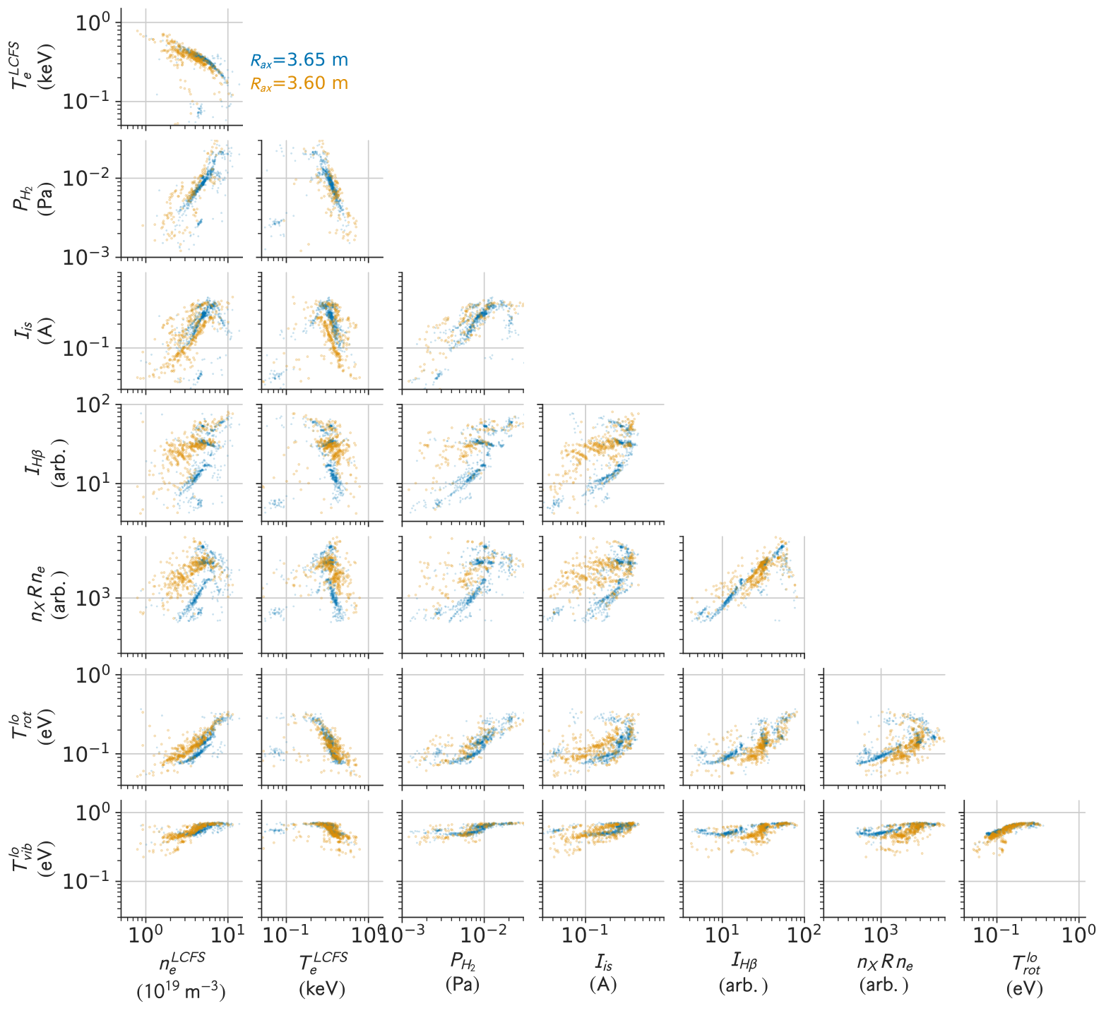
We collect the spectra obtained for 120 discharge experiments (74 experiments with = 3.65 m and 46 experiments with = 3.60 m) totalling 1145 frames. The summary of the experiments is shown in Table 2. There are also some variations in ECH and NBI powers. The same inference of the state population is carried out for all of these frames. Figure 6 shows the distribution among several parameters, , , , , , , , and at these frames. The parameters for the -m- and 3.60-m-experiments are shown in different colors.
| (m) | shotnumber | (T) | ECH (MW) | NBI |
| 3.65 | 142857-142917 | -2.712 | 75 | #1,2,3 |
| 143523-143560 | 2.712 | 60 | #1,2,3 | |
| 3.60 | 143293-143297 | -1.640 | 0 | #1,2,3,4,5 |
| 143306-143307 | -2.750 | 60 | #1,2,3,4,5 | |
| 143387-143415 | -2.750 | 60 | #1,2,3 | |
| 143943-143950 | -2.750 | 250-550 | #2,3 | |
| 143973-143988 | -2.750 | 75 | #2,3 |
4.1 Plasma parameters
varies over 0.06–, while varies 0.08–0.9 keV. has a negative correlation against . The values of and are dependent on each other, i.e., the most of the points in the top-left panel in Fig. 6 stay on a single curve. Positive correlations among , , and are apparent. This may be intuitive, as higher gas pressure often gives more dense plasma and dense plasmas often result in more ion flux to the divertor. However, the scatter plots show their diffuse relations compared with the - relation. This suggests that other factor also affects their relations. The similar trend can be seen in Fig. 2 (a), (b), where and changes accordingly, while the change in the and are not monotonic against the change of .
The values of and also show the positive correlations against . This is consistent with the positive correlation between and , i.e., the atom and molecule densities should have a positive dependence on and the emission rate is almost linearly proportional to . Their relations show a large scatter, suggesting existence of another process to affect the molecular density in front of the divertor.
4.2 The rotational temperature
The values of show a clear dependence on and . Expanded correlation plots are shown in Fig. 7. The scatter plot between and is closest to a single curve, while the scatter of - and - are larger. This suggests the direct dependence of the rotational temperature on the electron density, rather than the gas pressure and the ion flux to the divertor. This interpretation is consistent with that of the previous works [2, 30, 15]. However, it should be noted that we only consider the electron density at = 0.6 m and those exactly at the emission location are unavailable.
The solid curve in Fig. 7 (a) shows the empirical dependence of [24, 3, 15],
| (8) |
where is the surface temperature (assuming no extra excitation mechanism due to the surface recombination) in K, and is in . We assume the wall temperature at the desorption location as – K. The width of the curve shows this uncertainty. Although our result consistently shows the positive dependence with convergence to 600 K at , a significant discrepancy is found; our results lie at the larger density side of the solid curve. This discrepancy may be originated from the difference in and the values at the emission location.
In order to estimate the electron density on the divertor plate , we use the relation
| (9) |
which has been suggested in Ref. [17]. The dashed curves in Fig. 7 (a) show Eq. (8) but with this relation, the width of which again indicates – K. Our data point is in between the two curves. This may be understood that the dominant emission location is between the divertor plate and the LCFS. This is consistent with the emission location observation based on Zeeman spectroscopy in [10, 11].
4.3 The vibrational temperature
also shows a dependence on and . Expanded correlation plots are shown in Fig. 8. A similar positive -dependence of has been reported in [2]. From their plot, we extract the dependence as
| (10) |
with is again in . The solid curves in Fig. 8 (a) represent this relation, and the dashed curves show the same relation with the assumption of Eq. (9). The dependence of is in between the two curves. This is consistent with the above discussion for , where the emission location of the molecules is suggested between the divertor plate and the LCFS.
These observations for and indicate that Eq. (8) and Eq. (10) hold universally, although the geometry of the original experiment is different from that in this work; Brezinsek et al have measured the emission in front of the graphite limiter of TEXTOR [2], while we measured the emission from LHD divertor. This suggests that these parameters are mostly determined by the electron density, and the effect of the wall and electron / ion temperatures is small in this parameter range.
4.4 The other population parameters
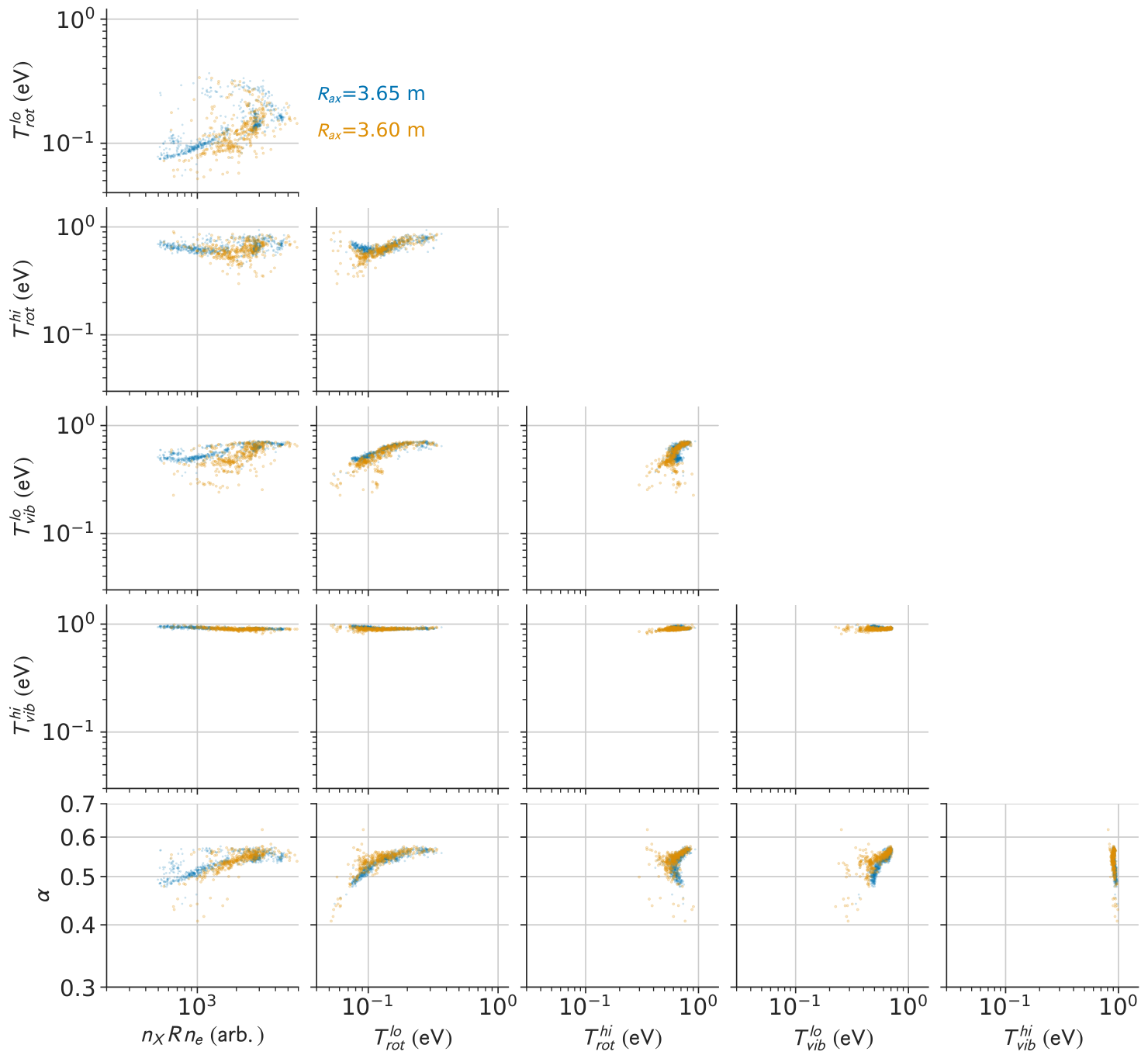
Correlation among the population parameters, , , , , , and , are shown in Fig. 9. and vary over the factor of 5 and 10, respectively. On the other hand, the variations of , , , and are smaller. For example, only changes by a factor of 1.5. Furthermore, the scatter plots among these population parameters except for show a significant correlation. For example, the pair plot of and (the top left panel) shows a large scatter, while - (the second panel from the top and the left) is close to a single curve. This suggests that a simple process determines the entire population distribution.
There are several processes have been proposed for the state population of hydrogen molecules, such as electron impact, proton impact, and neutral particle impact [22]. From Fig. 6, we see high correlation between and . On the other hand, the correlation between and shows larger scatter, although the -dependence of is known to small. This indicates that the dependence on is smaller, suggesting the unimportance of the molecular-collision effect on the population distribution. As such, a further study based on our data may help identification of important processes.
5 Conclusion
We analyzed a thousand visible spectra of Fulcher- band measured for divertor plasmas in the LHD. With the coronal model and Baysian inference, the population distribution of the electronical ground state was estimated from these spectra. A nearly linear -dependences of and were found, which is consistent with previous works. On the other hand, the higher rotational and vibrational temperatures as well as the mixture coefficient only show slight changes over the broad range of plasma parameters, and these parameters show a significant correlation. This suggests an importance of electron-impact excitation to determine the non-thermal population distribution of molecular hydrogen in divertor plasmas.
Appendix A Bayesian inference of the -state population
The two-temperature model we assume in Eq. (7) is not always robust. For example, the two temperature model has many optima that fit equally well for a single-temperature distribution; with any value of is one optimum, but with any value of is another optimum. In order to carry out a robust inference on the population parameters in Eq. (7) for thousands of frames, we utilized Bayesian inference framework. In this section, we show the details of the probabilistic model we have adopted in this work.
Let be the observed populations at the state and be its uncertainty from the measurement, where is the total numbef of frames and is the total number of molecular lines.for these spectra For each frame , we define the population parameters of the state, . Our aim is to infer the posterior distribution of with given the observation , .
With a given value of , we can compute the expected populations in the state based on Eq. (5). We assume the gaussian noise for with the standard deviation ,
| (11) |
where is the normal distribution with mean and the standard deviation . Here, we additionally assume the excess noise factore , which is a single parameter common for all the frames and upper states to capture the possible unidentified error in the measurement, e.g. overlap by other lines. is estimated and merginalized later.
We also assume prior distributions for the population parameters , which makes the inference robust. As a prior for , and , we assume the inverse gamma distribution, which is a typical distribution for a nonnegative random variable,
| (12) | ||||
| (13) | ||||
| (14) | ||||
| (15) | ||||
| (16) |
and for we assume beta distribution, which is a typical distribution for a variable in ,
| (17) |
where is the inverse gamma distribution with the shape parameter and the scale parameter with the gamma function. with the beta function . The hyperparameters, , , , , , , , , , are common for all the frames and will be inferred simultaneously. The graphical representation for our model is shown in Fig. 10.
Based on the Bayes rule, the posterior distribution can be found by integrating the hyperparameters,
| (18) |
where is the hyperprior distribution for . The inference (i.e., the integration) was carried out with Markov Chain Monte Carlo (MCMC) method with Stan Modeling Language [6, 25].
The median values of the hyperparameters are shown in Table 3. The prior distributions of and are shown in Fig. 7 (e) and Fig. 8 (e), respectively, by solid curves. The histogram of the estimated and are also shown in the same panel. It can be seen that these prior distributions are optimized so that they fit the entire distributions of and . In this panel, the median value as well as the % intervals are also shown.
| parameter | 16% – 50% – 84% | ||
|---|---|---|---|
| (eV) | 7.0 | 0.88 | 0.09 – 0.13 – 0.20 |
| (eV) | 4.5 | 0.47 – 0.67 – 1.01 | |
| (eV) | 20 | 12 | 0.49 – 0.61 – 0.77 |
| (eV) | 18 | 0.74 – 0.92 – 1.15 | |
| (arb.) | 0.85 | 3 | 2 – 6 – 30 |
| 36 | 54 | 0.35 – 0.40 – 0.45 |
acknowledgments
This work was supported by JSPS KAKENHI Grant Number 19K14680.
References
- [1] M. Bacal, A. M. Bruneteau, W. G. Graham, G. W. Hamilton, and M. Nachman. Pressure and electron temperature dependence of H density in a hydrogen plasma. Journal of Applied Physics, 52(3):1247–1254, March 1981.
- [2] S. Brezinsek, Ph. Mertens, A. Pospieszczyk, G. Sergienko, and P. T. Greenland. Molecular and Atomic Deuterium in the Plasma Edge of TEXTOR-94. Contributions to Plasma Physics, 42(6-7):668–674, November 2002.
- [3] S Brezinsek, G Sergienko, A Pospieszczyk, Ph Mertens, U Samm, and P T Greenland. Characterization of the deuterium recycling flux in front of a graphite surface in the TEXTOR tokamak. Plasma Phys. Controlled Fusion, 47(4):615, March 2005.
- [4] S. Briefi, D. Rauner, and U. Fantz. Determination of the rotational population of H2 and D2 including high-N states in low temperature plasmas via the Fulcher- transition. Journal of Quantitative Spectroscopy and Radiative Transfer, 187:135–144, jan 2017.
- [5] M. Capitelli and C. Gorse. Open problems in the physics of volume H/sup -//D/sup -/ sources. IEEE Transactions on Plasma Science, 33(6):1832–1844, December 2005.
- [6] Bob Carpenter, Andrew Gelman, Matthew D Hoffman, Daniel Lee, Ben Goodrich, Michael Betancourt, Marcus Brubaker, Jiqiang Guo, Peter Li, and Allen Riddell. Stan: A probabilistic programming language. Journal of statistical software, 76(1), 2017.
- [7] U Fantz, H Falter, P Franzen, D Wünderlich, M Berger, A Lorenz, W Kraus, P McNeely, R Riedl, and E Speth. Spectroscopy—a powerful diagnostic tool in source development. Nuclear Fusion, 46(6):S297–S306, June 2006.
- [8] U Fantz and B Heger. Spectroscopic diagnostics of the vibrational population in the ground state of and molecules. Plasma Physics and Controlled Fusion, 40(12):2023–2032, December 1998.
- [9] U. Fantz and D. Wünderlich. Franck-Condon factors, transition probabilities, and radiative lifetimes for hydrogen molecules and their isotopomeres. Atomic Data and Nuclear Data Tables, 92(6):853–973, November 2006.
- [10] K Fujii, T Shikama, M Goto, S Morita, and M Hasuo. Hydrogen transport diagnostics by atomic and molecular emission line profiles simultaneously measured for large helical device. Physics of plasmas, 20(1):012514, January 2013.
- [11] Keisuke Fujii, Keiji Sawada, Motoshi Goto, Shigeru Morita, and Masahiro Hasuo. Hydrogen atomic and molecular emission locations and intensities in the LHD edge plasma determined from simultaneously observed polarization spectra. Plasma and Fusion Research, 10:3402041–3402041, 2015.
- [12] O. Gabriel, D. C. Schram, and R. Engeln. Formation and relaxation of rovibrationally excited H 2 molecules due to plasma-surface interaction. Physical Review E, 78(1):016407, July 2008.
- [13] C. Gorse, R. Celiberto, M. Cacciatore, A. Laganá, and M. Capitelli. From dynamics to modeling of plasma complex systems: negative ion (H-) sources. Chemical Physics, 161(1-2):211–227, April 1992.
- [14] Masahiro Hasuo, Keisuke Fujii, Taiichi Shikama, Shigeru Morita, Motoshi Goto, and H Tanaka. Wideband High-Resolution spectroscopy on al-pellet ablation plasmas in large helical device. Journal of physics. Conference series, 397, 2012.
- [15] E M Hollmann, S Brezinsek, N H Brooks, M Groth, A G McLean, A Yu Pigarov, and D L Rudakov. Spectroscopic measurement of atomic and molecular deuterium fluxes in the DIII-D plasma edge. Plasma Phys. Controlled Fusion, 48(8):1165, July 2006.
- [16] Hiroki Ishihara, Arseniy Kuzmin, Masahiro Kobayashi, Taiichi Shikama, Keiji Sawada, Seiki Saito, Hiroaki Nakamura, Keisuke Fujii, and Masahiro Hasuo. Ro-vibrational population distribution in the ground state of hydrogen isotopologues in LHD peripheral plasmas deduced from emission spectroscopy. 267:107592.
- [17] M Kobayashi, Y Feng, S Morita, S Masuzaki, N Ezumi, T Kobayashi, M B Chowdhuri, H Yamada, T Morisaki, N Ohyabu, M Goto, I Yamada, K Narihara, A Komori, and O Motojima. Transport characteristics in the stochastic magnetic boundary of LHD: Magnetic field topology and its impact on divertor physics and impurity transport. Fusion Science and Technology, 58(1):220–231, August 2010.
- [18] S.I. Krasheninnikov, A.Yu. Pigarov, T.K. Soboleva, and D.J. Sigmar. Plasma-neutral gas interaction in a tokamak divertor: Effects of hydrogen molecules and plasma recombination. Journal of Nuclear Materials, 241-243:283–287, February 1997.
- [19] Chr May, M Baelmans, and P BiSrner. Non-linear effects on neutral gas transport in divertors. page 7.
- [20] M. Péalat, J-P. E. Taran, M. Bacal, and F. Hillion. Rovibrational molecular populations, atoms, and negative ions in H and D magnetic multicusp discharges. The Journal of Chemical Physics, 82(11):4943–4953, June 1985.
- [21] Keiji Sawada, Kouji Eriguchi, and Takashi Fujimoto. Hydrogen-atom spectroscopy of the ionizing plasma containing molecular hydrogen: Line intensities and ionization rate. Journal of Applied Physics, 73(12):8122–8125, jun 1993.
- [22] Keiji Sawada and Motoshi Goto. Rovibrationally Resolved Time-Dependent Collisional-Radiative Model of Molecular Hydrogen and Its Application to a Fusion Detached Plasma. Atoms, 4(4):29, December 2016.
- [23] Keiji Sawada, Hiroaki Nakamura, Seiki Saito, Gakushi Kawamura, Masahiro Kobayashi, Kenta Haga, Ryusei Migita, Takumi Sawada, and Masahiro Hasuo. Neutral transport code for rovibrational population calculation of molecular hydrogen in large helical device plasmas. Contrib. Plasma Phys., 60(5-6):e201900153, June 2020.
- [24] G Sergienko, G Arnoux, S Brezinsek, M Clever, A Huber, U Kruezi, A G Meigs, Ph Mertens, U Samm, and M Stamp. Molecular deuterium behaviour in tungsten divertor on JET. J. Nucl. Mater., 438:S1100–S1103, 2013.
- [25] Stan Development Team. PyStan: the python interface to Stan, 2022. Python package version 3.4.0.
- [26] G. C. Stutzin, A. T. Young, H. F. Döbele, A. S. Schlachter, K. N. Leung, and W. B. Kunkel. In situ density and temperature measurements of vibrationally excited hydrogen molecules in ion source plasmas. Review of Scientific Instruments, 61(1):619–621, January 1990.
- [27] G C Stutzin, A T Young, A S Schlachter, K N Leung, and W B Kunkel. In situ measurement of rovibrational populations of H2 ground electronic state in a plasma by VUV laser absorption. Chem. Phys. Lett., 155(4):475–480, March 1989.
- [28] Elizabeth Surrey and Brendan Crowley. Spectroscopic measurement of gas temperature in the neutralizer of the JET neutral beam injection system. Plasma Phys. Controlled Fusion, 45(7):1209, June 2003.
- [29] Hirotaka Tanaka, Keisuke Fujii, Taiichi Shikama, Shigeru Morita, Motoshi Goto, and Masahiro Hasuo. Plasma spectroscopy on an Aluminum-Pellet ablation cloud in an LHD plasma with an echelle spectrometer. Atoms for Peace, an International Journal, 8(4):81, November 2020.
- [30] B. Unterberg, S. Brezinsek, G. Sergienko, C.C. Chu, P. Dumortier, J.D. Hey, D. Kalupin, A. Kreter, M. Lehnen, A.M. Messiaen, Ph. Mertens, A. Pospieszczyk, U. Samm, B. Schweer, M.Z. Tokar’, and G. Van Wassenhove. Local effects of gas fuelling and their impact on transport processes in the plasma edge of the tokamak TEXTOR. Journal of Nuclear Materials, 337-339:515–519, March 2005.
- [31] P. Vankan, D.C. Schram, and R. Engeln. High rotational excitation of molecular hydrogen in plasmas. Chemical Physics Letters, 400(1-3):196–200, December 2004.
- [32] E Watts, G O Sitz, D A McCormack, G J Kroes, R A Olsen, J A Groeneveld, J N P Van Stralen, E J Baerends, and R C Mowrey. Rovibrationally inelastic scattering of (v=1, j=1) H2 from cu(100): Experiment and theory. J. Chem. Phys., 114(1):495–503, January 2001.
- [33] Bingjia Xiao, Shinichiro Kado, Shin Kajita, and Daisuke Yamasaki. Rovibrational distribution determination of H in low temperature plasmas by Fulcher- band spectroscopy. Plasma Physics and Controlled Fusion, 46(4):653–668, April 2004.