跳到论文正文
W Papers独立论文阅读器 arXiv:2302.08449 论文正文 计算阅读时间 · 0%
引用这篇论文根据当前论文元数据生成,正式投稿前建议核对。


License: arXiv.org perpetual non-exclusive license
arXiv:2302.08449v3 [math.AP] 19 Nov 2023

Multiscale modelling and analysis of growth of plant tissues

Arezki Boudaoud, Annamaria Kiss, Mariya Ptashnyk
LadHyX, CNRS, Ecole Polytechnique, IP Paris, Palaiseau, France
RDP, ENS de Lyon, Claude Bernard University Lyon 1, CNRS, INRAE, Lyon, France
Department of Mathematics, Heriot-Watt University, The Maxwell Institute for Mathematical Sciences, Edinburgh, Scotland, UK
Abstract.

How morphogenesis depends on cell properties is an active direction of research. Here, we focus on mechanical models of growing plant tissues, where microscopic (sub)cellular structure is taken into account. In order to establish links between microscopic and macroscopic tissue properties, we perform a multiscale analysis of a model of growing plant tissue with subcellular resolution. We use homogenization to rigorously derive the corresponding macroscopic tissue scale model. Tissue scale mechanical properties are computed from microscopic structural and material properties, taking into account deformation by the growth field. We then consider case studies and numerically compare the detailed microscopic model and the tissue-scale model, both implemented using finite element method. We find that the macroscopic model can be used to efficiently make predictions about several configurations of interest. Our work will help making links between microscopic measurements and macroscopic observations in growing tissues.

1. Introduction

Modelling plant growth and morphogenesis is an active area of research [53]. A major difficulty in this area is that growth is ‘inherently a multiscale process’ [53], bridging subcellular to organ scales. Each plant cell is surrounded by a thin layer of polysaccharides, known as the cell wall, and exerts on this wall a hydrodynamic pressure, termed turgor pressure. Plant cell growth is driven by turgor pressure and restrained by the cell wall. Organ morphogenesis results from specific spatial distributions of growth rates across cells and tissues. As a consequence, the form of an organ is dependent on all processes occurring from sub-wall scale to supra-cellular scale, raising the need for multiscale modelling approaches.

Most previous modelling effort has focused on one scale or one process at a time. For instance, several studies have addressed how cell wall rheology emerges from its composition, microstructure, and/or synthesis [7, 19, 20, 28, 44]. These studies adopted approaches from continuum mechanics and used partial differential equations (PDEs) to describe the cell wall as an anisotropic material, with different assumptions on the rheology – viscous [19, 20], elastic [7, 8, 44, 47], or viscoelastoplastic [28]; growth then corresponds to flow of the viscous material or to remodelling of the elastic material, combined with synthesis of new material. Other studies represented tissues as tessellations by polygons of 2D space or of surfaces embedded in 3D that describe the position of vertices, relying on high-dimensional systems of ordinary differential equations [7, 15, 24, 31, 35]. The authors investigated how tissue shape changes according to cell wall rheology, assuming for instance each edge to be a viscoelastoplastic element, or to how mechanical stress in tissues feeds back on cell wall dynamics. Other studies used continuous, PDE-based approaches for modelling tissue dynamics and investigated how patterns of tissue mechanical properties or of growth potential yield organ morphogenesis [26, 54], see the comprehensive overview in [22].

In this context, a systematic derivation of macroscopic (supra-cellular) tissue rheology from (sub)wall rheology is still lacking. Here we try to address this issue using multiscale modelling and homogenization techniques. There are many results on homogenization of equations of linear elasticity, e.g. [4, 14, 29, 43, 45, 50], however to our knowledge the multiscale analysis of the two-way coupling between elastic deformation and growth presented in here is novel.

In the derivation of the microscopic model we start from the framework of morphoelasticity [23, 49]. Following [49], we consider the multiplicative decomposition of the deformation gradient into elastic and growth part and model elastic deformations of plant cell walls using equations of linearised elasticity. To describe the growth we use Lockhart’s law [32] that relates plant cell wall growth with deformation gradient and accounts for microscopic subwall properties. Along with modelling growth processes, the multiplicative decomposition approach is also used in multiscale modelling and analysis of plastic deformations, where the decomposition corresponds to the elastic and plastic deformations respectively, e.g. [16, 36, 39]. Rigorous well-posedness results were recently obtained for a model combining multiplicative decomposition and nonlinear elasticity [17].

Applying homogenization techniques, the two-scale convergence [3, 41] and periodic unfolding [11, 13] methods, we rigorously derive macroscopic equations that describe elastic deformations and growth at the tissue scale. In particular, we provide explicit formulae for macroscopic elastic properties as a function of microscopic parameters and microscopic structure. An important step in the rigorous derivation of the macroscopic problem is the proof of the strong convergence of the sequence of growth and strain tensors as the small parameter, representing a ratio between the size of the microstructure and the size of the tissue, converges to zero. We illustrate our results by solving numerically the corresponding microscopic and macroscopic equations and analyse the degree of agreement between solutions of the macroscopic problem and solutions of the original microscopic model defined at the cell wall scale. An important contribution to the numerical simulation of the macroscopic two-scale problem is the development of a two-scale numerical algorithm that allows an efficient coupling between macroscopic and microscopic properties and processes. Along with numerical efficiency, the advantage of the derivation of macroscopic tissue level models for plant growth allow us to study different biological settings which are difficult or even impossible to formulate and simulate at the cell-scale level.

The paper is organized as follows. In section 2 we formulate and analyse the microscopic model for plant tissue growth. The macroscopic model is derived in sections 3 using both formal asymptotic expansion and rigorous derivation applying the two-scale convergence and the periodic unfolding methods. Description of the numerical simulation algorithm and implementation of the numerical methods is given in section 4. In section 5 we present numerical simulation results, followed by a short conclusion and an appendix.

2. Derivation of microscopic model for plant tissue growth

In our mathematical model for the growth of a plant tissue we consider a microscopic geometry of a plant tissue composed of cells surrounded by cell walls, connected by middle lamella, see specific geometry in Figure 1a-b. In modelling the dynamics of plant tissue we consider the elastic deformations and growth of these cell walls and middle lamella.

By Ωt⊂ℝd\Omega_{t}\subset\mathbb{R}^{d}, with t>0t>0 and d=2d=2 or 33, we shall represent a part of a plant tissue in the current configuration at time tt and ∂Ωt\partial\Omega_{t} denotes the external boundary of the tissue. We shall consider the growth and elastic deformation of a plant tissue given by the map χ⁡(t,⋅):Ω→ℝd\chi(t,\cdot):\Omega\to\mathbb{R}^{d} from the initial (reference) configuration Ω⊂ℝd\Omega\subset\mathbb{R}^{d} into deformed (current) configuration Ωt=χ⁡(t,Ω)\Omega_{t}=\chi(t,\Omega) of a plant tissue for t>0t>0. We consider Ω\Omega to be a bounded Lipschitz convex or a bounded C1,γ~C^{1,\tilde{\gamma}}, with γ~∈(0,1)\tilde{\gamma}\in(0,1), domain.

When modelling growth we use the framework of morphoelasticity and consider the multiplicative decomposition of the deformation gradient 𝐅=𝐈+∇𝐮{\bf F}={\bf I}+\nabla{\bf u} into elastic and growth parts 𝐅=𝐅e​𝐅g{\bf F}={\bf F}_{e}{\bf F}_{g}, where 𝐮{\bf u} is the displacement of the cell walls and middle lamella according to the map χ\chi and 𝐅e{\bf F}_{\rm e} and 𝐅g{\bf F}_{\rm g} are elastic and growth deformation gradients, respectively. Then the elastic strain is given by

(1) 𝐄el=12​(𝐅eT​𝐅e−𝐈)=12​[(𝐅e−𝐈)T​(𝐅e−𝐈)+(𝐅e−𝐈)+(𝐅e−𝐈)T]\displaystyle{\bf E}^{\rm el}=\frac{1}{2}({\bf F}^{T}_{\rm e}{\bf F}_{\rm e}-{\bf I})=\frac{1}{2}[({\bf F}_{{\rm e}}-{\bf I})^{T}({\bf F}_{{\rm e}}-{\bf I})+({\bf F}_{{\rm e}}-{\bf I})+({\bf F}_{{\rm e}}-{\bf I})^{T}]
=12​[(𝐅e−𝐈)T​(𝐅e−𝐈)+(𝐈+∇𝐮)​𝐅g−1+((𝐈+∇𝐮)​𝐅g−1)T−2​𝐈].\displaystyle=\frac{1}{2}[({\bf F}_{{\rm e}}-{\bf I})^{T}({\bf F}_{{\rm e}}-{\bf I})+({\bf I}+\nabla{\bf u}){\bf F}_{\rm g}^{-1}+(({\bf I}+\nabla{\bf u}){\bf F}_{{\rm g}}^{-1})^{T}-2{\bf I}].

We model the cell walls and middle lamella as an hyperelastic material and consider the stress tensor in the form

𝝈⁡(x,𝐅e)=Je−1​𝐅e​∂𝐅eW​(x,𝐅e)T,{\boldsymbol{\sigma}}(x,{\bf F}_{\rm e})=J_{\rm e}^{-1}{\bf F}_{\rm e}\partial_{{\bf F}_{\rm e}}W(x,{\bf F}_{\rm e})^{T},

where WW is the strain energy function and Je=det⁡(𝐅e)=det⁡(𝐅𝐅g−1)J_{\rm e}={\rm det}({\bf F}_{\rm e})={\rm det}({\bf F}{\bf F}_{g}^{-1}). Then the constitutive equation for elastic deformations is given by

𝝈⁡(x,𝐅e)=𝝈⁡(x,∇𝐮,𝐅g−1)=Je−1​𝐅𝐅g−1​∂𝐅eW​(x,𝐅𝐅g−1)T.{\boldsymbol{\sigma}}(x,{\bf F}_{\rm e})={\boldsymbol{\sigma}}(x,\nabla{\bf u},{\bf F}_{\rm g}^{-1})=J_{\rm e}^{-1}{\bf F}{\bf F}_{\rm g}^{-1}\partial_{{\bf F}_{\rm e}}W(x,{\bf F}{\bf F}_{\rm g}^{-1})^{T}.

Mechanical equilibrium requires that

(2) −divx~​𝝈​(x,∇𝐮,𝐅g−1)=0 in ​Ωtw,t>0,-{\rm div}_{\tilde{x}}\,{\boldsymbol{\sigma}}(x,\nabla{\bf u},{\bf F}_{\rm g}^{-1})=0\quad\text{ in }\;\Omega^{w}_{t},\;t>0,

where Ωtw\Omega^{w}_{t} denotes the domain of cell walls and middle lamellae, joining the walls of individual cells together, and x~\tilde{x} denotes the coordinates in the current configuration. We complete equations (2) with the boundary conditions

(3) 𝝈⁡(x,∇𝐮,𝐅g−1)​ν\displaystyle{\boldsymbol{\sigma}}(x,\nabla{\bf u},{\bf F}_{\rm g}^{-1})\nu =−P​ν\displaystyle=-P\nu on ​Γt,t>0,\displaystyle\text{ on }\;\Gamma_{t},\;t>0,
𝝈⁡(x,∇𝐮,𝐅g−1)​ν\displaystyle{\boldsymbol{\sigma}}(x,\nabla{\bf u},{\bf F}_{\rm g}^{-1})\nu =𝐟\displaystyle={\bf f} on ​∂Ωt∖ΓD,t,t>0,\displaystyle\text{ on }\;\partial\Omega_{t}\setminus\Gamma_{D,t},\;t>0,
𝐮⋅ν=0,Πτ​(𝝈⁡(x,∇𝐮,𝐅g−1)​ν)=0\displaystyle{\bf u}\cdot\nu=0,\;\;\Pi_{\tau}\big({\boldsymbol{\sigma}}(x,\nabla{\bf u},{\bf F}_{\rm g}^{-1})\nu\big)=0 or 𝐮=0\displaystyle\text{ or }\quad{\bf u}=0 on ​ΓD,t,t>0,\displaystyle\text{ on }\;\Gamma_{D,t},\;t>0,

where PP is the turgor pressure inside the cells which can vary between cells and across the tissue, 𝐟{\bf f} denotes external forces, ν\nu is the external normal vector to the boundaries of Ωtw\Omega_{t}^{w} in current configuration, Γt\Gamma_{t} denotes the boundary of cells, corresponding to plasma membranes, ΓD,t⊂∂Ωt\Gamma_{D,t}\subset\partial\Omega_{t} for t≥0t\geq 0, and Πτ\Pi_{\tau} denotes the tangential components of the corresponding vector.

We can rewrite (2) and (3), defined in the current configuration, in the reference configuration to obtain

(4) −div⁡(Jg​𝐒T​(x,∇𝐮,𝐅g−1)​𝐅g−T)\displaystyle-{\rm div}(J_{\rm g}\,{\bf S}^{T}(x,\nabla{\bf u},{\bf F}_{\rm g}^{-1})\,{\bf F}_{\rm g}^{-T}) =0\displaystyle=0\quad in ​Ωw,t>0,\displaystyle\text{ in }\;\Omega^{w},\;t>0,
Jg​𝐒T​(x,∇𝐮,𝐅g−1)​𝐅g−T​N\displaystyle J_{\rm g}\,{\bf S}^{T}(x,\nabla{\bf u},{\bf F}_{\rm g}^{-1}){\bf F}_{\rm g}^{-T}N =−J​P​𝐅−T​N\displaystyle=-J\,P\,{\bf F}^{-T}N on ​Γ,t>0,\displaystyle\text{ on }\;\Gamma,\;t>0,
Jg​𝐒T​(x,∇𝐮,𝐅g−1)​𝐅g−T​N\displaystyle J_{\rm g}\,{\bf S}^{T}(x,\nabla{\bf u},{\bf F}_{\rm g}^{-1}){\bf F}_{\rm g}^{-T}N =𝐟​J​|𝐅−T​N|\displaystyle={\bf f}\,J\,|{\bf F}^{-T}N| on ​∂Ω∖ΓD,t>0,\displaystyle\text{ on }\;\partial\Omega\setminus\Gamma_{D},\;t>0,
𝐮⋅N=0,Πτ​(Jg​𝐒T​(x,∇𝐮,𝐅g−1)​𝐅g−T​N)=0\displaystyle{\bf u}\cdot N=0,\;\;\Pi_{\tau}\big(J_{\rm g}\,{\bf S}^{T}(x,\nabla{\bf u},{\bf F}_{\rm g}^{-1}){\bf F}_{\rm g}^{-T}N\big)=0 or 𝐮=0\displaystyle\text{ or }\quad{\bf u}=0 on ​ΓD,t>0,\displaystyle\text{ on }\;\Gamma_{D},\;t>0,

where NN denotes the external normal vector to the boundaries of the reference domain of cell walls and middle lamella Ωw⊂ℝd\Omega^{w}\subset\mathbb{R}^{d}, and the nominal elastic stress is given by

𝐒T​(x,∇𝐮,𝐅g−1)=∂𝐅eW⁡(x,𝐅𝐅g−1).{\bf S}^{T}(x,\nabla{\bf u},{\bf F}_{\rm g}^{-1})=\partial_{{\bf F}_{\rm e}}W(x,{\bf F}{\bf F}_{\rm g}^{-1}).

To specify the constitutive relation for the stress tensor 𝝈\boldsymbol{\sigma}, or correspondent nominal tensor 𝐒{\bf S}, we assume small elastic strain (small elastic deformations of plant tissues), i.e.

𝝈⁡(x,∇𝐮,𝐅g−1)≈𝐒T​(x,∇𝐮,𝐅g−1)≈𝔼⁡(x)​𝜺el​(∇𝐮,𝐅g−1),\boldsymbol{\sigma}(x,\nabla{\bf u},{\bf F}_{\rm g}^{-1})\approx{\bf S}^{T}(x,\nabla{\bf u},{\bf F}_{\rm g}^{-1})\approx{\mathbb{E}}(x){\boldsymbol{\varepsilon}}^{\rm el}(\nabla{\bf u},{\bf F}_{\rm g}^{-1}),

where 𝔼⁡(x)=∂𝐅e∂𝐅eW⁡(x,𝟏)\mathbb{E}(x)=\partial_{{\bf F}_{\rm e}}\partial_{{\bf F}_{\rm e}}W(x,{\bf 1}) is the elasticity tensor and 𝜺el\boldsymbol{\varepsilon}^{\rm el} is the linearised version of the elastic strain (1), which depends on the displacement gradient and growth tensor

𝜺el(∇𝐮,𝐅g−1)=12[∇𝐮𝐅g−1+(∇𝐮𝐅g−1)T+𝐅g−1+𝐅g−T−2𝐈]=sym(∇𝐮𝐅g−1)+sym(𝐅g−1)−𝐈.{\boldsymbol{\varepsilon}}^{\rm el}(\nabla{\bf u},{\bf F}_{\rm g}^{-1})=\frac{1}{2}\big[\nabla{\bf u}\,{\bf F}_{\rm g}^{-1}+(\nabla{\bf u}\,{\bf F}_{\rm g}^{-1})^{T}+{\bf F}_{\rm g}^{-1}+{\bf F}_{\rm g}^{-T}-2{\bf I}\big]={\rm sym}(\nabla{\bf u}\,{\bf F}_{\rm g}^{-1})+{\rm sym}({\bf F}_{\rm g}^{-1})-{\bf I}.

We also assume J​𝐅−T≈Jg​𝐅g−TJ{\bf F}^{-T}\approx J_{g}{\bf F}_{\rm g}^{-T} for small elastic strain. Notice that for 𝐅g=𝐈{\bf F}_{\rm g}={\bf I} we recover the standard formula for the strain in the case of linear elasticity.

To complete the model we specify equation for the growth tensor 𝐅g{\bf F}_{\rm g}

(5) ∂𝐅g∂t=G⁡(x,∇𝐮,𝐅g−1)​𝐅g\displaystyle\frac{\partial{\bf F}_{\rm g}}{\partial t}=G(x,\nabla{\bf u},{\bf F}_{\rm g}^{-1})\,{\bf F}_{\rm g} in ​Ωw,t>0,\displaystyle\text{ in }\;\Omega^{w},\;\;t>0,
𝐅g​(0,x)=𝐈\displaystyle\bf{\displaystyle F}_{\rm g}(0,x)={\bf I} for ​x∈Ωw.\displaystyle\text{ for }\,x\in\Omega^{w}.

Since there is no consensus on modelling growth [22, 53], we consider two scenarii and assume that the growth depends on the local average of stress or of strain in cell walls and middle lamella (both are compatible with Lockhart’s law [32]). We also assume that the cell wall and middle lamella expand when the local average of the stress or strain is larger than some threshold value [32]. Hence we consider the stress based growth

G~​(x,∇𝐮,𝐅g−1)=G~​(x,𝝈⁡(x,∇𝐮,𝐅g−1))=ησ​[𝝈^−𝝉σ]+,\tilde{G}(x,\nabla{\bf u},{\bf F}_{\rm g}^{-1})=\tilde{G}(x,\boldsymbol{\sigma}(x,\nabla{\bf u},{\bf F}_{\rm g}^{-1}))=\eta_{\sigma}[{\boldsymbol{\hat{\sigma}}}-\boldsymbol{\tau}_{\sigma}]_{+},

or the elastic strain based growth

G~​(x,∇𝐮,𝐅g−1)=G~​(x,𝜺el​(∇𝐮,𝐅g−1))=ηε​[𝜺^el−𝝉ε]+,\tilde{G}(x,\nabla{\bf u},{\bf F}_{\rm g}^{-1})=\tilde{G}(x,{\boldsymbol{\varepsilon}}^{\rm el}(\nabla{\bf u},{\bf F}_{\rm g}^{-1}))=\eta_{\varepsilon}[\boldsymbol{\hat{\varepsilon}}^{\rm el}-{\boldsymbol{\tau}}_{\varepsilon}]_{+},

and

(6) G​(x,∇𝐮,𝐅g−1)i​j={−M if ​G~​(x,∇𝐮,𝐅g−1)i​j≤−M,G~​(x,∇𝐮,𝐅g−1)i​j if −M<G~​(x,∇𝐮,𝐅g−1)i​j<M,M if ​G~​(x,∇𝐮,𝐅g−1)i​j≥M,for ​i,j=1,…,d,G(x,\nabla{\bf u},{\bf F}_{\rm g}^{-1})_{ij}=\begin{cases}-M&\text{ if }\;\tilde{G}(x,\nabla{\bf u},{\bf F}_{\rm g}^{-1})_{ij}\leq-M,\\ \tilde{G}(x,\nabla{\bf u},{\bf F}_{\rm g}^{-1})_{ij}&\text{ if }\;-M<\tilde{G}(x,\nabla{\bf u},{\bf F}_{\rm g}^{-1})_{ij}<M,\\ M&\text{ if }\;\tilde{G}(x,\nabla{\bf u},{\bf F}_{\rm g}^{-1})_{ij}\geq M,\end{cases}\quad\text{for }\;i,j=1,\ldots,d,

for some M>0M>0. Here [v]+=QT​[D​v]+​Q[v]_{+}=Q^{T}[Dv]^{+}Q with QQ the rotation that diagonalizes the tensor vv, and [D​v]+[Dv]^{+} is a diagonal matrix with the positive parts of the eigenvalues of vv on its diagonal. This allows to relate growth only to tensile stress, in the case of stress based growth, or only to elongational strain, in the case of strain based growth. The uniform boundedness assumption on the growth rate GG is used in the rigorous analysis of the model and is not restrictive from the biological point of view. Notice that in the growth laws we consider piece-wise constant fields 𝝈^\boldsymbol{\hat{\sigma}} and 𝜺^el\boldsymbol{\hat{\varepsilon}}^{\rm el}, obtained as an average over each cell of 𝝈\boldsymbol{\sigma} and 𝜺el\boldsymbol{\varepsilon}^{\rm el} respectively. The growth laws introduce two physical parameters: the extensibility constants ησ\eta_{\sigma} and ηε\eta_{\varepsilon} and threshold matrices 𝝉σ{\boldsymbol{\tau}}_{\sigma} and 𝝉ε{\boldsymbol{\tau}}_{\varepsilon}, respectively.

2.1. Formulation of the microscopic model

We assume that in a plant tissue cells are distributed periodically and consider the parameter δ>0\delta>0 that determines the ratio between the size of a cell and the size of the tissue. We also assume that the size of the cell and the thickness of the cell wall hh are of the same order and much smaller than the size of the tissue, i.e. δ\delta is small. To define the microscopic structure of the plant tissue given by the cell walls and middle lamella, we consider a ‘unit cell’ YY and Yc⊂YY_{c}\subset Y represents the voids filled by biological cells, with Lipschitz boundary Γ=∂Yc\Gamma=\partial Y_{c} and composed of a finite number of subdomains separated from each other and from the edges of YY, whereas Yw=Y∖Y¯cY_{w}=Y\setminus\overline{Y}_{c} represents cell walls surrounded by middle lamella. Then the microscopic geometry of a plant tissue in the reference configuration is defined as

Ωcδ=⋃ξ∈Ξδδ⁡(Y¯c+ξ)​ and ​Ωδ=Ω∖Ωcδ,\Omega_{c}^{\delta}=\bigcup_{\xi\in\Xi_{\delta}}\delta\,(\overline{Y}_{c}+\xi)\;\;\text{ and }\;\;\Omega^{\delta}=\Omega\setminus\Omega_{c}^{\delta},

where Ξδ={ξ∈Ξ:δ(Y¯+ξ)⊂Ω¯,dist(δ(Y¯c+ξ),∂Ω)≥κδ}\Xi_{\delta}=\{\xi\in\Xi:\delta\,(\overline{Y}+\xi)\subset\overline{\Omega},\,{\rm dist}(\delta\,(\overline{Y}_{c}+\xi),\partial\Omega)\geq\kappa\delta\} and Ξ={ξ∈ℝd:ξ=∑j=1dkjbj,k∈ℤd}\Xi=\{\xi\in\mathbb{R}^{d}:\xi=\sum_{j=1}^{d}k_{j}b_{j},\,k\in\mathbb{Z}^{d}\}, with {bj}j=1d\{b_{j}\}_{j=1}^{d} being the basis vectors of YY, i.e. Y={y∈ℝd:y=∑j=1dsjbj,s∈(0,1)d}Y=\{y\in\mathbb{R}^{d}:y=\sum_{j=1}^{d}s_{j}b_{j},\,s\in(0,1)^{d}\}, and for some fixed κ>0\kappa>0. The boundaries of Ωδ\Omega^{\delta} that correspond to cell plasma-membranes are

Γδ=⋃ξ∈Ξδδ⁡(Γ+ξ) and Γδ=∂Ωδ∖∂Ω.\Gamma^{\delta}=\bigcup_{\xi\in\Xi_{\delta}}\delta\,(\Gamma+\xi)\quad\text{ and }\quad\Gamma^{\delta}=\partial\Omega^{\delta}\setminus\partial\Omega.

The parts of the tissues near the boundary ∂Ω\partial\Omega, which do not include the complete δ​Y¯\delta\,\overline{Y} are denoted by

Λδ=Ω∖⋃ξ∈Ξδδ⁡(Y¯+ξ)​ and ​Λδ=⋃l=1LΛδl, with ​Λδl∩δ⁡(Y+ξ)≠∅​ for one ​ξ∈Ξ​ and ​L=𝒪⁡(1/δd−1).\Lambda_{\delta}=\Omega\setminus\bigcup_{\xi\in\Xi_{\delta}}\delta\,(\overline{Y}+\xi)\;\text{ and }\;\Lambda_{\delta}=\bigcup_{l=1}^{L}\Lambda^{l}_{\delta},\;\text{ with }\;\Lambda^{l}_{\delta}\cap\delta\,(Y+\xi)\neq\emptyset\;\text{ for one }\;\xi\in\Xi\;\text{ and }\;L=\mathcal{O}(1/\delta^{d-1}).

Then microscopic equations for elastic deformations in the reference domain read

(7) −div⁡(Jgδ​𝐒δT​(x,∇𝐮δ,𝐅g,δ−1)​𝐅g,δ−T)\displaystyle-{\rm div}(J_{\rm g}^{\delta}\,{\bf S}^{T}_{\delta}(x,\nabla{\bf u}^{\delta},{\bf F}_{{\rm g},\delta}^{-1})\,{\bf F}_{{\rm g},\delta}^{-T}) =0\displaystyle=0\quad in ​Ωδ,t>0,\displaystyle\text{ in }\;\Omega^{\delta},\;t>0,
Jgδ​𝐒δT​(x,∇𝐮δ,𝐅g,δ−1)​𝐅g,δ−T​N\displaystyle J_{\rm g}^{\delta}\,{\bf S}_{\delta}^{T}(x,\nabla{\bf u}^{\delta},{\bf F}_{{\rm g},\delta}^{-1})\,{\bf F}_{{\rm g},\delta}^{-T}N =−Jgδ​Pδ​(t,x)​𝐅g,δ−T​N\displaystyle=-J_{\rm g}^{\delta}\,P^{\delta}(t,x){\bf F}_{{\rm g},\delta}^{-T}N on ​Γδ,t>0,\displaystyle\text{ on }\;\Gamma^{\delta},\;t>0,
Jgδ​𝐒δT​(x,∇𝐮δ,𝐅g,δ−1)​𝐅g,δ−T​N\displaystyle J_{\rm g}^{\delta}\,{\bf S}_{\delta}^{T}(x,\nabla{\bf u}^{\delta},{\bf F}_{{\rm g},\delta}^{-1})\,{\bf F}_{{\rm g},\delta}^{-T}N =Jgδ​𝐟​(t,x)​|𝐅g,δ−T​N|\displaystyle=J_{\rm g}^{\delta}\,{\bf f}(t,x)\,|{\bf F}_{{\rm g},\delta}^{-T}N| on ​∂Ω∖ΓD,t>0,\displaystyle\text{ on }\;\partial\Omega\setminus\Gamma_{D},\;t>0,
𝐮δ⋅N=0,Πτ​(Jgδ​𝐒δT​(x,∇𝐮δ,𝐅g,δ−1)​𝐅g,δ−T​N)=0\displaystyle{\bf u}^{\delta}\cdot N=0,\;\;\Pi_{\tau}\big(J_{\rm g}^{\delta}\,{\bf S}_{\delta}^{T}(x,\nabla{\bf u}^{\delta},{\bf F}_{{\rm g},\delta}^{-1})\,{\bf F}_{{\rm g},\delta}^{-T}N\big)=0 or 𝐮δ=0\displaystyle\text{ or }\quad{\bf u}^{\delta}=0 on ​ΓD,t>0,\displaystyle\text{ on }\;\Gamma_{D},\;t>0,

where Jgδ=det⁡(𝐅g,δ)J_{\rm g}^{\delta}={\rm det}({\bf F}_{{\rm g},\delta}), 𝐒δT(x,∇𝐮δ,𝐅g,δ−1)=𝔼δ(x)𝜺el(∇𝐮δ,𝐅g,δ−1)=𝔼δ(x)[sym(∇𝐮δ𝐅g,δ−1)+sym(𝐅g,δ−1)−𝐈]{\bf S}_{\delta}^{T}(x,\nabla{\bf u}^{\delta},{\bf F}_{{\rm g},\delta}^{-1})=\mathbb{E}^{\delta}(x){\boldsymbol{\varepsilon}}^{\rm el}(\nabla{\bf u}^{\delta},{\bf F}_{{\rm g},\delta}^{-1})=\mathbb{E}^{\delta}(x)[{\rm sym}(\nabla{\bf u}^{\delta}{\bf F}_{{\rm g},\delta}^{-1})+{\rm sym}({\bf F}_{{\rm g},\delta}^{-1})-{\bf I}], with 𝔼δ​(x)=𝔼⁡(x,x/δ)\mathbb{E}^{\delta}(x)=\mathbb{E}(x,x/\delta), and Pδ​(t,x)=P⁡(t,x,x/δ)P^{\delta}(t,x)=P(t,x,x/\delta) for given functions 𝔼:Ω×Y→ℝ4​d\mathbb{E}:\Omega\times Y\to\mathbb{R}^{4d} and P:(0,T)×Ω×Γ→ℝP:(0,T)\times\Omega\times\Gamma\to\mathbb{R}, extended YY-periodically to ℝd\mathbb{R}^{d} and to ⋃ξ∈Ξ(Γ+ξ)\bigcup_{\xi\in\Xi}(\Gamma+\xi) respectively.

The dynamics of the growth tensor is determined by

(8) ∂𝐅g,δ∂t=Gδ​(x,∇𝐮δ,𝐅g,δ−1)​𝐅g,δ\displaystyle\frac{\partial{\bf F}_{{\rm g},\delta}}{\partial t}=G^{\delta}(x,\nabla{\bf u}^{\delta},{\bf F}_{{\rm g},\delta}^{-1})\,{\bf F}_{{\rm g},\delta}\quad in ​Ωδ,t>0,\displaystyle\text{ in }\;\Omega^{\delta},\;\;t>0,
𝐅g,δ​(0,x)=𝐈\displaystyle\bf{\displaystyle F}_{{\rm g},\delta}(0,x)={\bf I} in ​Ωδ,\displaystyle\text{ in }\;\Omega^{\delta},

where

G~δ​(x,∇𝐮δ,𝐅g,δ−1)\displaystyle\tilde{G}^{\delta}(x,\nabla{\bf u}^{\delta},{\bf F}_{{\rm g},\delta}^{-1}) =ησ[−∫δ⁡([x/δ]Y+Yw)∩Ω𝝈(x~,∇𝐮δ,𝐅g,δ−1)dx~−𝝉σ]+\displaystyle=\eta_{\sigma}\Big[\mathchoice{{\vbox{\hbox{$\textstyle-$}}\kern-5.05557pt}}{{\vbox{\hbox{$\scriptstyle-$}}\kern-3.56781pt}}{{\vbox{\hbox{$\scriptscriptstyle-$}}\kern-3.02435pt}}{{\vbox{\hbox{$\scriptscriptstyle-$}}\kern-2.87088pt}}\!\int_{\delta([x/\delta]_{Y}+Y_{w})\cap\Omega}{\boldsymbol{\sigma}}(\tilde{x},\nabla{\bf u}^{\delta},{\bf F}_{{\rm g},\delta}^{-1})\,d\tilde{x}-{\boldsymbol{\tau}}_{\sigma}\Big]_{+}  or\displaystyle\qquad\text{ or }
G~δ​(x,∇𝐮δ,𝐅g,δ−1)\displaystyle\tilde{G}^{\delta}(x,\nabla{\bf u}^{\delta},{\bf F}_{{\rm g},\delta}^{-1}) =ηε[−∫δ⁡([x/δ]Y+Yw)∩Ω𝜺el(∇𝐮δ,𝐅g,δ−1)dx~−𝝉ε]+,\displaystyle=\eta_{\varepsilon}\Big[\mathchoice{{\vbox{\hbox{$\textstyle-$}}\kern-5.05557pt}}{{\vbox{\hbox{$\scriptstyle-$}}\kern-3.56781pt}}{{\vbox{\hbox{$\scriptscriptstyle-$}}\kern-3.02435pt}}{{\vbox{\hbox{$\scriptscriptstyle-$}}\kern-2.87088pt}}\!\int_{\delta([x/\delta]_{Y}+Y_{w})\cap\Omega}{\boldsymbol{\varepsilon}}^{\rm el}(\nabla{\bf u}^{\delta},{\bf F}_{{\rm g},\delta}^{-1})\,d\tilde{x}-{\boldsymbol{\tau}}_{\varepsilon}\Big]_{+},

with 𝝈⁡(x,∇𝐮δ,𝐅g,δ−1)=𝐒δT​(x,∇𝐮δ,𝐅g,δ−1)=𝔼δ​(x)​𝜺el​(∇𝐮δ,𝐅g,δ−1){\boldsymbol{\sigma}}(x,\nabla{\bf u}^{\delta},{\bf F}_{{\rm g},\delta}^{-1})={\bf S}^{T}_{\delta}(x,\nabla{\bf u}^{\delta},{\bf F}_{{\rm g},\delta}^{-1})=\mathbb{E}^{\delta}(x){\boldsymbol{\varepsilon}}^{\rm el}(\nabla{\bf u}^{\delta},{\bf F}_{{\rm g},\delta}^{-1}), and

(9) Gδ​(x,∇𝐮δ,𝐅g,δ−1)i​j={−M if G~δ​(x,∇𝐮δ,𝐅g,δ−1)i​j≤−M,G~δ​(x,∇𝐮δ,𝐅g,δ−1)i​j if −M<G~δ​(x,∇𝐮δ,𝐅g,δ−1)i​j<M,M if G~δ​(x,∇𝐮δ,𝐅g,δ−1)i​j≥M, for ​i,j=1,…,d.G^{\delta}(x,\nabla{\bf u}^{\delta},{\bf F}_{{\rm g},\delta}^{-1})_{ij}=\begin{cases}-M&\text{ if }\;\qquad\quad\tilde{G}^{\delta}(x,\nabla{\bf u}^{\delta},{\bf F}_{{\rm g},\delta}^{-1})_{ij}\leq-M,\\ \tilde{G}^{\delta}(x,\nabla{\bf u}^{\delta},{\bf F}_{{\rm g},\delta}^{-1})_{ij}&\text{ if }\;-M<\tilde{G}^{\delta}(x,\nabla{\bf u}^{\delta},{\bf F}_{{\rm g},\delta}^{-1})_{ij}<M,\\ M&\text{ if }\;\qquad\quad\tilde{G}^{\delta}(x,\nabla{\bf u}^{\delta},{\bf F}_{{\rm g},\delta}^{-1})_{ij}\geq M,\end{cases}\qquad\text{ for }i,j=1,\ldots,d.

2.2. Well-posedness of microscopic model

To prove existence of a weak solution of problem (7) and (8), we consider standard ellipticity assumptions on the elasticity tensor 𝔼\mathbb{E} and regularity assumptions on the pressure PδP^{\delta} and boundary forces 𝐟{\bf f}. For the pressure inside of the cells PδP^{\delta} we shall consider dependence on the microscopic structure in the form

(10) Pδ​(t,x)=P1​(t,x)+δ​P2​(t,x,x/δ),P^{\delta}(t,x)=P_{1}(t,x)+\delta P_{2}(t,x,x/\delta),

for some given functions P1:(0,T)×Ω→ℝP_{1}:(0,T)\times\Omega\to\mathbb{R} and P2:(0,T)×Ω×Γ→ℝP_{2}:(0,T)\times\Omega\times\Gamma\to\mathbb{R}.

Assumption 2.1.
  • •

    Elasticity tensor 𝔼∈Cγ​(Ω¯,Lper∞​(Y))4​d\mathbb{E}\in C^{\gamma}(\overline{\Omega};L^{\infty}_{\rm per}(Y))^{4d} is positive definite and bounded, i.e. α1​|𝐀|2≤𝔼⁡(x,y)​𝐀⋅𝐀≤α2​|𝐀|2\alpha_{1}|{\bf A}|^{2}\leq\mathbb{E}(x,y){\bf A}\cdot{\bf A}\leq\alpha_{2}|{\bf A}|^{2} for x∈Ωx\in\Omega, y∈Yy\in Y, symmetric matrices 𝐀∈ℝd×d{\bf A}\in\mathbb{R}^{d\times d}, and positive constants α1,α2\alpha_{1},\alpha_{2}, and has minor and major symmetries, i.e. 𝔼i​j​k​l=𝔼k​l​i​j=𝔼j​i​k​l=𝔼i​j​l​k\mathbb{E}_{ijkl}=\mathbb{E}_{klij}=\mathbb{E}_{jikl}=\mathbb{E}_{ijlk}, for i,j,k,l=1,…,di,j,k,l=1,\ldots,d,   for γ∈(0,1)\gamma\in(0,1).

  • •

    𝐟∈Cγ​([0,T]×∂Ω){\bf f}\in C^{\gamma}([0,T]\times\partial\Omega), P1∈Cγ​([0,T],C1​(Ω¯))P_{1}\in C^{\gamma}([0,T];C^{1}(\overline{\Omega})) and P2∈Cγ​([0,T]×Ω¯×Γ)P_{2}\in C^{\gamma}([0,T]\times\overline{\Omega}\times\Gamma), where P2(t,x,⋅)P_{2}(t,x,\cdot) is YY-periodically extended to Γ+ξ\Gamma+\xi, with ξ∈Ξ\xi\in\Xi, for γ∈(0,1)\gamma\in(0,1).

If ΓD≠∅\Gamma_{D}\neq\emptyset, consider 𝒢\mathcal{G} the symmetry group of ΓD\Gamma_{D}, formed of at most one, for d=2d=2, or two, for d=3d=3, translations and at most one rotation, for d=3d=3, that leave ΓD\Gamma_{D} invariant. Let 𝒢τ\mathcal{G}_{\tau} be the subspace of ℝd{\mathbb{R}}^{d} spanned by the set of translations in 𝒢\mathcal{G} and {𝝆1,𝝆2}\{\boldsymbol{\rho}_{1},\boldsymbol{\rho}_{2}\} be the orthonormal basis of the plane perpendicular to the rotation axis. Then, depending on the boundary conditions, we define the following space for solutions of (7)

Vδ=\displaystyle V_{\delta}= {𝐮∈H1​(Ωδ)d:𝐮=0​ on ​ΓD} or\displaystyle\{{\bf u}\in H^{1}(\Omega^{\delta})^{d}\,:\;{\bf u}=0\,\text{ on }\,\Gamma_{D}\}\qquad\qquad\text{ or }
Vδ=\displaystyle V_{\delta}= {𝐮∈H1(Ωδ)d:𝐮⋅N=0 on ΓD,∫ΩδΠ𝒢τ(𝐮)dx=0,∫Ω𝝆1(∇𝐮^−∇𝐮^T)𝝆2dx=0},\displaystyle\{{\bf u}\in H^{1}(\Omega^{\delta})^{d}\,:\;{\bf u}\cdot N=0\,\text{ on }\,\Gamma_{D},\;\int_{\Omega^{\delta}}\Pi_{\mathcal{G}_{\tau}}({\bf u})\,dx=0,\,\,\int_{\Omega}\boldsymbol{\rho}_{1}(\nabla\hat{\bf u}-\nabla\hat{\bf u}^{T})\boldsymbol{\rho}_{2}\,dx=0\},

where Π𝒢τ\Pi_{\mathcal{G}_{\tau}} is the projection on 𝒢τ\mathcal{G}_{\tau} and 𝐮^\hat{\bf u} denotes an extension of 𝐮{\bf u} from Ωδ\Omega^{\delta} into Ω\Omega, see e.g. [42]. If ΓD=∅\Gamma_{D}=\emptyset, then

Vδ={𝐮∈H1(Ωδ)d:∫Ωδ𝐮dx=0,∫Ω(∂xj𝐮^i−∂xi𝐮^j)dx=0, for i≠j,i,j=1,…,d}.V_{\delta}=\{{\bf u}\in H^{1}(\Omega^{\delta})^{d}\;:\int_{\Omega^{\delta}}{\bf u}\,dx=0,\;\int_{\Omega}\big(\partial_{x_{j}}\hat{\bf u}_{i}-\partial_{x_{i}}\hat{\bf u}_{j}\big)dx=0,\;\text{ for }i\neq j,\;i,j=1,\ldots,d\}.

Using (10) for PδP^{\delta} and div⁡(Jgδ​𝐅g,δ−T)=0{\rm div}(J_{\rm g}^{\delta}{\bf F}_{{\rm g},\delta}^{-T})=0 in Ωδ\Omega^{\delta} we can rewrite equations in (7) as

(11) −div⁡(Jgδ​(𝐒δT​(x,∇𝐮δ,𝐅g,δ−1)+P1​(t,x)​𝐈)​𝐅g,δ−T)\displaystyle-{\rm div}\Big(J_{\rm g}^{\delta}\,\Big({\bf S}^{T}_{\delta}(x,\nabla{\bf u}^{\delta},{\bf F}_{{\rm g},\delta}^{-1})+P_{1}(t,x){\bf I}\Big)\,{\bf F}_{{\rm g},\delta}^{-T}\Big) =−Jgδ𝐅g,δ−T∇P1(t,x)\displaystyle=-J_{\rm g}^{\delta}{\bf F}_{{\rm g},\delta}^{-T}\nabla P_{1}(t,x)\quad in ​Ωδ,t>0,\displaystyle\text{ in }\Omega^{\delta},\;t>0,
Jgδ​(𝐒δT​(x,∇𝐮δ,𝐅g,δ−1)+P1​(t,x)​𝐈)​𝐅g,δ−T​N\displaystyle J_{\rm g}^{\delta}\,\Big({\bf S}_{\delta}^{T}(x,\nabla{\bf u}^{\delta},{\bf F}_{{\rm g},\delta}^{-1})+P_{1}(t,x){\bf I}\Big)\,{\bf F}_{{\rm g},\delta}^{-T}N =−δ​Jgδ​P2δ​(t,x)​𝐅g,δ−T​N\displaystyle=-\delta\,J_{\rm g}^{\delta}\,P_{2}^{\delta}(t,x){\bf F}_{{\rm g},\delta}^{-T}N on ​Γδ,t>0,\displaystyle\text{ on }\Gamma^{\delta},\;t>0,
Jgδ​𝐒δT​(x,∇𝐮δ,𝐅g,δ−1)​𝐅g,δ−T​N\displaystyle J_{\rm g}^{\delta}\,{\bf S}_{\delta}^{T}(x,\nabla{\bf u}^{\delta},{\bf F}_{{\rm g},\delta}^{-1})\,{\bf F}_{{\rm g},\delta}^{-T}N =Jgδ​𝐟​(t,x)​|𝐅g,δ−T​N|\displaystyle=J_{\rm g}^{\delta}\,{\bf f}(t,x)|{\bf F}_{{\rm g},\delta}^{-T}N| on ​ΓN,t>0,\displaystyle\text{ on }\Gamma_{N},\;t>0,
𝐮δ⋅N=0,Jgδ​Πτ​(𝐒δT​(x,∇𝐮δ,𝐅g,δ−1)​𝐅g,δ−T​N)=0\displaystyle{\bf u}^{\delta}\cdot N=0,\;J_{\rm g}^{\delta}\,\Pi_{\tau}\big({\bf S}_{\delta}^{T}(x,\nabla{\bf u}^{\delta},{\bf F}_{{\rm g},\delta}^{-1})\,{\bf F}_{{\rm g},\delta}^{-T}N\big)=0 or 𝐮δ=0\displaystyle\text{ or }\quad{\bf u}^{\delta}=0 on ​ΓD,t>0,\displaystyle\text{ on }\Gamma_{D},\;t>0,

where ΓN=∂Ω∖ΓD\Gamma_{N}=\partial\Omega\setminus\Gamma_{D} and P2δ​(t,x)=P2​(t,x,x/δ)P_{2}^{\delta}(t,x)=P_{2}(t,x,x/\delta).

In the analysis and numerical implementation of (8) and (11) we shall consider weak solutions of the model equations. We shall use the notation ⟨ϕ,ψ⟩A=∫Aϕ​ψ​𝑑x\langle\phi,\psi\rangle_{A}=\int_{A}\phi\psi\,dx, for ϕ∈Lp​(A)\phi\in L^{p}(A), ψ∈Lq​(A)\psi\in L^{q}(A), and ⟨ϕ,ψ⟩∂A=∫∂Aϕ​ψ​𝑑γ\langle\phi,\psi\rangle_{\partial A}=\int_{\partial A}\phi\psi\,d\gamma, for ϕ∈Lp​(∂A)\phi\in L^{p}(\partial A), ψ∈Lq​(∂A)\psi\in L^{q}(\partial A), with 1<p,q<∞1<p,q<\infty, 1/p+1/q=11/p+1/q=1, and a bounded Lipschitz domain AA.

Definition 2.2.

A weak solution of (8) and (11) are 𝐮δ∈L2​(0,T,Vδ){\bf u}^{\delta}\in L^{2}(0,T;V_{\delta}) and 𝐅g,δ∈W1,∞​(0,T,Lq​(Ωδ))d×d{\bf F}_{{\rm g},\delta}\in W^{1,\infty}(0,T;L^{q}(\Omega^{\delta}))^{d\times d}, for any q∈(1,∞)q\in(1,\infty), with 𝐅g,δ∈L∞​((0,T)×Ωδ)d×d{\bf F}_{{\rm g},\delta}\in L^{\infty}((0,T)\times\Omega^{\delta})^{d\times d}, satisfying

(12) ⟨Jgδ𝔼δ(x)sym(∇𝐮δ𝐅g,δ−1)+P1(t,x)𝐈,∇φ𝐅g,δ−1⟩Ωδ+δ⟨JgδP2δ(t,x)𝐅g,δ−TN,φ⟩Γδ\displaystyle\Big\langle J_{\rm g}^{\delta}\,\mathbb{E}^{\delta}(x){\rm sym}(\nabla{\bf u}^{\delta}{\bf F}_{{\rm g},\delta}^{-1})+P_{1}(t,x){\bf I},\nabla\varphi{\bf F}_{{\rm g},\delta}^{-1}\Big\rangle_{\Omega^{\delta}}+\delta\,\Big\langle J_{{\rm g}}^{\delta}\,P_{2}^{\delta}(t,x)\,{\bf F}_{{\rm g},\delta}^{-T}N,\varphi\Big\rangle_{\Gamma^{\delta}}
−⟨JgδP1(t,x)𝐅g,δ−TN,φ⟩∂Ω=⟨Jgδ𝔼δ(x)[𝐈−sym(𝐅g,δ−1)],∇φ𝐅g,δ−1⟩Ωδ\displaystyle-\Big\langle J_{{\rm g}}^{\delta}\,P_{1}(t,x)\,{\bf F}_{{\rm g},\delta}^{-T}N,\varphi\Big\rangle_{\partial\Omega}=\Big\langle J_{\rm g}^{\delta}\,\mathbb{E}^{\delta}(x)\big[{\bf I}-{\rm sym}({\bf F}_{{\rm g},\delta}^{-1})\big],\nabla\varphi{\bf F}_{{\rm g},\delta}^{-1}\Big\rangle_{\Omega^{\delta}}
−⟨Jgδ𝐅g,δ−T∇P1(t,x),φ⟩Ωδ+⟨Jgδ𝐟(t,x)|𝐅g,δ−TN|,φ⟩ΓN\displaystyle-\Big\langle J_{\rm g}^{\delta}\,{\bf F}_{{\rm g},\delta}^{-T}\nabla P_{1}(t,x),\varphi\Big\rangle_{\Omega^{\delta}}+\Big\langle J_{\rm g}^{\delta}\,{\bf f}(t,x)\,|{\bf F}_{{\rm g},\delta}^{-T}N|,\varphi\Big\rangle_{\Gamma_{N}}

for φ∈L2​(0,T,Vδ)\varphi\in L^{2}(0,T;V_{\delta}) and a.a. t∈(0,T)t\in(0,T), and 𝐅g,δ{\bf F}_{{\rm g},\delta} satisfies (8) a.e. in (0,T)×Ωδ(0,T)\times\Omega^{\delta}.

First we shall prove a version of the Korn inequality, where the symmetric gradient includes the growth tensor.

Lemma 2.3.

For 𝐮∈Vδ{\bf u}\in V_{\delta} and a tensor 𝐅∈L∞​(Ω){\bf F}\in L^{\infty}(\Omega) such that on each δ⁡(Y+ξ)∩Ω\delta(Y+\xi)\cap\Omega, for ξ∈Ξ\xi\in\Xi, 𝐅{\bf F} is constant, det⁡(𝐅)≥1{\rm det}({\bf F})\geq 1 and eigenvalues λj​(𝐅)≥1\lambda_{j}({\bf F})\geq 1 for j=1,…,dj=1,\ldots,d, we have the following estimate

(13) ‖𝐮‖L2​(Ωδ)2+‖∇𝐮‖L2​(Ωδ)2≤C​‖sym⁡(∇𝐮𝐅−1)‖L2​(Ωδ)2,\|{\bf u}\|^{2}_{L^{2}(\Omega^{\delta})}+\|\nabla{\bf u}\|^{2}_{L^{2}(\Omega^{\delta})}\leq C\|{\rm{sym}}\big(\nabla{\bf u}{\bf F}^{-1}\big)\|^{2}_{L^{2}(\Omega^{\delta})},

with constant C=C⁡(𝐅)C=C({\bf F}) independent of δ\delta.

Proof.

Assumptions on the microscopic structure of the plant tissues ensure the existence of an extension 𝐮^\hat{\bf u} of 𝐮{\bf u} from Ωδ\Omega^{\delta} to Ω\Omega with

‖𝐮^‖H1​(Ω)\displaystyle\|\hat{\bf u}\|_{H^{1}(\Omega)} ≤C∥𝐮∥H1​(Ωδ),\displaystyle\leq C\|{\bf u}\|_{H^{1}(\Omega^{\delta})},\quad ‖𝐮^‖L2​(Ω)+‖sym⁡(∇𝐮^)‖L2​(Ω)\displaystyle\|\hat{\bf u}\|_{L^{2}(\Omega)}+\|{\rm{sym}}(\nabla\hat{\bf u})\|_{L^{2}(\Omega)} ≤C⁡(‖𝐮‖L2​(Ωδ)+‖sym⁡(∇𝐮)‖L2​(Ωδ)),\displaystyle\leq C\big(\|{\bf u}\|_{L^{2}(\Omega^{\delta})}+\|{\rm{sym}}(\nabla{\bf u})\|_{L^{2}(\Omega^{\delta})}\big),
‖∇𝐮^‖L2​(Ω)\displaystyle\|\nabla\hat{\bf u}\|_{L^{2}(\Omega)} ≤C∥∇𝐮∥L2​(Ωδ),\displaystyle\leq C\|\nabla{\bf u}\|_{L^{2}(\Omega^{\delta})},\quad ‖sym⁡(∇𝐮^)‖L2​(Ω)\displaystyle\|{\rm{sym}}(\nabla\hat{\bf u})\|_{L^{2}(\Omega)} ≤C​‖sym⁡(∇𝐮)‖L2​(Ωδ),\displaystyle\leq C\|{\rm{sym}}(\nabla{\bf u})\|_{L^{2}(\Omega^{\delta})},

where constant CC is independent of δ\delta, see e.g. [42]. In the following we shall identify 𝐮{\bf u} with its extension 𝐮^\hat{\bf u}. Using that 𝐅{\bf F} and hence 𝐅−T{\bf F}^{-T} are constant on each δ⁡(Y+ξ)∩Ω\delta(Y+\xi)\cap\Omega, for ξ∈Ξ\xi\in\Xi, and the properties of Ωδ\Omega^{\delta}, together with an extension of 𝐮{\bf u} from δ​𝐅​(ξ)​Yw\delta{\bf F}(\xi)Y_{w} into δ​𝐅​(ξ)​Y\delta{\bf F}(\xi)Y, constructed as in e.g. [42, Lemma 4.1], we obtain

∫Ωδ|sym⁡(∇𝐮𝐅−1)|2​𝑑x=∑ξ∈Ξδ∫δ⁡(Yw+ξ)|sym⁡(∇𝐮𝐅−1)|2​𝑑x+∑l=1L∫Λδl|sym⁡(∇𝐮𝐅−1)|2​𝑑x\displaystyle\int_{\Omega^{\delta}}|{\rm{sym}}(\nabla{\bf u}{\bf F}^{-1})|^{2}dx=\sum_{\xi\in\Xi_{\delta}}\int_{\delta(Y_{w}+\xi)}|{\rm{sym}}(\nabla{\bf u}{\bf F}^{-1})|^{2}dx+\sum_{l=1}^{L}\int_{\Lambda_{\delta}^{l}}|{\rm{sym}}(\nabla{\bf u}{\bf F}^{-1})|^{2}dx
=∑ξ∈Ξδdet⁡(𝐅−1​(ξ))​∫δ​𝐅​(ξ)​(Yw+ξ)|sym⁡(∇𝐮)|2​𝑑x+∑l=1Ldet⁡(𝐅−1​(ξl))​∫𝐅⁡(ξl)​Λδl|sym⁡(∇𝐮)|2​𝑑x\displaystyle=\sum_{\xi\in\Xi_{\delta}}{\rm det}({\bf F}^{-1}(\xi))\int_{\delta{\bf F}(\xi)(Y_{w}+\xi)}|{\rm{sym}}(\nabla{\bf u})|^{2}dx+\sum_{l=1}^{L}{\rm det}({\bf F}^{-1}(\xi_{l}))\int_{{\bf F}(\xi_{l})\Lambda_{\delta}^{l}}|{\rm{sym}}(\nabla{\bf u})|^{2}dx
≥∑ξ∈Ξδdet⁡(𝐅−1​(ξ))​C​(𝐅⁡(ξ))​∫δ​𝐅​(ξ)​(Y+ξ)|sym⁡(∇𝐮)|2​dx+∑l=1Ldet⁡(𝐅−1​(ξl))​∫𝐅⁡(ξl)​Λδl|sym⁡(∇𝐮)|2​dx,\displaystyle\geq\sum_{\xi\in\Xi_{\delta}}{\rm det}({\bf F}^{-1}(\xi))C({\bf F}(\xi))\int_{\delta{\bf F}(\xi)(Y+\xi)}|{\rm{sym}}(\nabla{\bf u})|^{2}dx+\sum_{l=1}^{L}{\rm det}({\bf F}^{-1}(\xi_{l}))\int_{{\bf F}(\xi_{l})\Lambda_{\delta}^{l}}|{\rm{sym}}(\nabla{\bf u})|^{2}dx,

where the dependence of the constant CC on 𝐅⁡(ξ){\bf F}(\xi), for ξ∈Ξδ\xi\in\Xi_{\delta}, arises from the application of the Korn and Poincaré inequalities when constructing an extension from 𝐅⁡(ξ)​Yw{\bf F}(\xi)Y_{w} into 𝐅⁡(ξ)​Y{\bf F}(\xi)Y, see [42, Lemma 4.1] for more details, and ξl∈Λδl\xi_{l}\in\Lambda_{\delta}^{l} for l=1,…,Ll=1,\ldots,L. Using the uniform boundedness of 𝐅{\bf F}, together with the fact that det⁡(𝐅)≥1{\rm det}({\bf F})\geq 1 in (0,T)×Ω(0,T)\times\Omega and eigenvalues λj​(𝐅)≥1\lambda_{j}({\bf F})\geq 1, with j=1,…,dj=1,\ldots,d, and applying the Korn inequality, see e.g. [10, 18, 42], yield

∫Ωδ|sym⁡(∇𝐮𝐅−1)|2​𝑑x\displaystyle\int_{\Omega^{\delta}}|{\rm sym}(\nabla{\bf u}{\bf F}^{-1})|^{2}dx ≥C​∫ΩF|sym⁡(∇𝐮)|2​𝑑x≥C​∫Ω|sym⁡(∇𝐮)|2​𝑑x\displaystyle\geq C\int_{\Omega_{F}}|{\rm sym}(\nabla{\bf u})|^{2}dx\geq C\int_{\Omega}|{\rm sym}(\nabla{\bf u})|^{2}dx
≥C​∫Ω(|𝐮|2+|∇𝐮|2)​dx≥C​∫Ωδ(|𝐮|2+|∇𝐮|2)​dx,\displaystyle\geq C\int_{\Omega}\big(|{\bf u}|^{2}+|\nabla{\bf u}|^{2}\big)dx\geq C\int_{\Omega^{\delta}}(\big|{\bf u}|^{2}+|\nabla{\bf u}|^{2}\big)dx,

for 𝐮∈Vδ{\bf u}\in V_{\delta}, where ΩF=(⋃ξ∈Ξδδ​𝐅​(ξ)​(Y+ξ))​⋃(⋃l=1L𝐅⁡(ξl)​Λδl)\Omega_{F}=\big(\bigcup_{\xi\in\Xi_{\delta}}\delta{\bf F}(\xi)(Y+\xi)\big)\bigcup\big(\bigcup_{l=1}^{L}{\bf F}(\xi_{l})\Lambda_{\delta}^{l}\big). This implies the result stated in the lemma. ∎

Remark 2.1.

Some results on the generalisation of the Korn inequality can be found in [38, 46]. Notice that in [38] C1C^{1}-regularity of 𝐅{\bf F} is required and in [46] the continuity of 𝐅{\bf F} or 𝐮=0{\bf u}=0 on ∂Ω\partial\Omega are assumed. In the proof of Lemma 2.3 we use the fact that 𝐅{\bf F} is uniformly bounded and piece-wise constant and the eigenvalues of 𝐅{\bf F} satisfy λj​(𝐅)≥1\lambda_{j}({\bf F})\geq 1, for j=1,…,dj=1,\ldots,d, ensuring that Ω\Omega is a subdomain of the transformed domain ΩF\Omega_{F}.

Using the inequality (13) and applying the Banach fixed point theorem we prove the well-posedness result for microscopic model (8) and (11).

Theorem 2.4.

Under Assumptions 2.1 there exists a unique weak solution of (8), (11) satisfying

(14) ‖𝐮δ‖L∞​(0,T,Vδ)+‖𝐅g,δ‖L∞​((0,T)×Ωδ)+‖∂t𝐅g,δ‖L∞​((0,T)×Ωδ)+‖𝐅g,δ‖W1,∞​(0,T,Lq​(Ωδ))≤C,\|{\bf u}^{\delta}\|_{L^{\infty}(0,T;V_{\delta})}+\|{\bf F}_{\rm g,\delta}\|_{L^{\infty}((0,T)\times\Omega^{\delta})}+\|\partial_{t}{\bf F}_{\rm g,\delta}\|_{L^{\infty}((0,T)\times\Omega^{\delta})}+\|{\bf F}_{\rm g,\delta}\|_{W^{1,\infty}(0,T;L^{q}(\Omega^{\delta}))}\leq C,

with a constant CC independent of δ\delta and any q∈(1,∞)q\in(1,\infty).

Proof.

We shall apply a fixed point argument to show existence of a solution of (8), (11). Consider

𝒲=\displaystyle\mathcal{W}= {𝐅∈L∞((0,T)×Ωδ)d×d:𝐅∈W1,∞(0,T;Lq(Ωδ))d×d,∥𝐅∥L∞​((0,T)×Ωδ)≤κ^,det(𝐅)≥1,\displaystyle\{{\bf F}\in L^{\infty}((0,T)\times\Omega^{\delta})^{d\times d}:{\bf F}\in W^{1,\infty}(0,T;L^{q}(\Omega^{\delta}))^{d\times d},\;\|{\bf F}\|_{L^{\infty}((0,T)\times\Omega^{\delta})}\leq\hat{\kappa},\;{\rm det}({\bf F})\geq 1,\;
λj(𝐅)≥1 in [0,T]×Ωδ,j=1,…d, and piece-wise constant in each δ(Yw+ξ)∩Ω for ξ∈Ξ},\displaystyle\lambda_{j}({\bf F})\geq 1\text{ in }[0,T]\times\Omega^{\delta},j=1,\ldots d,\text{ and piece-wise constant in each }\delta(Y_{w}+\xi)\cap\Omega\;\text{ for }\;\xi\in\Xi\},

with κ^≥exp⁡(d​M​T)\hat{\kappa}\geq\exp(dMT). For a given 𝐅~g,δ∈𝒲\tilde{\bf F}_{{\rm g},\delta}\in\mathcal{W}, taking 𝐮δ{\bf u}^{\delta} as a test function in (12) and using assumptions on 𝔼\mathbb{E}, P1P_{1}, P2P_{2}, and 𝐟{\bf f}, together with the fact that 1≤det⁡(𝐅~g,δ)≤C1\leq{\rm det}(\tilde{\bf F}_{{\rm g},\delta})\leq C, with a constant CC independent of δ\delta, we obtain

(15) ∥sym(∇𝐮δ𝐅~g,δ−1)∥L∞​(0,T,L2​(Ωδ))2≤C(1+ς∥𝐮δ∥L∞​(0,T,Vδ)2),\|{\rm{sym}}(\nabla{\bf u}^{\delta}\tilde{\bf F}_{{\rm g},\delta}^{-1})\|^{2}_{L^{\infty}(0,T;L^{2}(\Omega^{\delta}))}\leq C\big(1+\varsigma\|{\bf u}^{\delta}\|^{2}_{L^{\infty}(0,T;V_{\delta})}\big),

for any fixed ς>0\varsigma>0. Here we also used the trace estimate

δ​‖v‖L2​(Γδ)2≤C⁡(‖v‖L2​(Ωδ)2+δ2​‖∇v‖L2​(Ωδ)2) for ​v∈H1​(Ωδ),\delta\|v\|^{2}_{L^{2}(\Gamma^{\delta})}\leq C\big(\|v\|^{2}_{L^{2}(\Omega^{\delta})}+\delta^{2}\|\nabla v\|^{2}_{L^{2}(\Omega^{\delta})}\big)\quad\text{ for }\;v\in H^{1}(\Omega^{\delta}),

for some constant CC independent of δ\delta, see e.g. [27]. Notice that since 𝐅~g,δ\tilde{\bf F}_{{\rm g},\delta} is constant on each δ⁡(Yw+ξ)∩Ω\delta(Y_{w}+\xi)\cap\Omega it can be trivially extended by the constant into each δ⁡(Y+ξ)∩Ω\delta(Y+\xi)\cap\Omega, for ξ∈Ξ\xi\in\Xi. Using Lemma 2.3 we obtain

(16) ∥𝐮δ∥L∞​(0,T,Vδ)≤C∥sym(∇𝐮δ𝐅~g,δ−1)∥L∞​(0,T,L2​(Ωδ)),\|{\bf u}^{\delta}\|_{L^{\infty}(0,T;V_{\delta})}\leq C\|{\rm{sym}}(\nabla{\bf u}^{\delta}\tilde{\bf F}_{{\rm g},\delta}^{-1})\|_{L^{\infty}(0,T;L^{2}(\Omega^{\delta}))},

and then choosing in (15) sufficiently small ς>0\varsigma>0 yields

(17) ‖𝐮δ‖L∞​(0,T,Vδ)≤C,\|{\bf u}^{\delta}\|_{L^{\infty}(0,T;V_{\delta})}\leq C,

where the constant CC does not depend on δ\delta. Assumptions on 𝔼\mathbb{E}, P1,P2P_{1},P_{2}, 𝐟{\bf f} and 𝐅~g,δ\tilde{\bf F}_{{\rm g},\delta}, together with the estimate in Lemma 2.3, ensure that

F⁡(φ)=\displaystyle F(\varphi)= ⟨JgδP1(t,x)𝐅~g,δ−TN,φ⟩∂Ω−⟨P1(t,x)𝐈,∇φ𝐅~g,δ−1⟩Ωδ−δ⟨JgδP2δ(t,x)𝐅~g,δ−TN,φ⟩Γδ\displaystyle\Big\langle J_{{\rm g}}^{\delta}\,P_{1}(t,x)\,\tilde{\bf F}_{{\rm g},\delta}^{-T}N,\varphi\Big\rangle_{\partial\Omega}-\Big\langle P_{1}(t,x){\bf I},\nabla\varphi\,\tilde{\bf F}_{{\rm g},\delta}^{-1}\Big\rangle_{\Omega^{\delta}}-\delta\Big\langle J_{{\rm g}}^{\delta}\,P_{2}^{\delta}(t,x)\,\tilde{\bf F}_{{\rm g},\delta}^{-T}N,\varphi\Big\rangle_{\Gamma^{\delta}}
+⟨Jgδ𝔼δ(x)[𝐈−sym(𝐅~g,δ−1)],∇φ𝐅~g,δ−1⟩Ωδ−⟨Jgδ𝐅~g,δ−T∇P1(t,x),φ⟩Ωδ+⟨Jgδ𝐟(t,x)|𝐅~g,δ−TN|,φ⟩ΓN\displaystyle+\Big\langle J_{\rm g}^{\delta}\,\mathbb{E}^{\delta}(x)\big[{\bf I}-{\rm sym}(\tilde{\bf F}_{{\rm g},\delta}^{-1})\big],\nabla\varphi\,\tilde{\bf F}_{{\rm g},\delta}^{-1}\Big\rangle_{\Omega^{\delta}}-\Big\langle J_{\rm g}^{\delta}\,\tilde{\bf F}_{{\rm g},\delta}^{-T}\nabla P_{1}(t,x),\varphi\Big\rangle_{\Omega^{\delta}}+\Big\langle J_{\rm g}^{\delta}\,{\bf f}(t,x)\,|\tilde{\bf F}_{{\rm g},\delta}^{-T}N|,\varphi\Big\rangle_{\Gamma_{N}}

defines a bounded linear functional on VδV_{\delta} and

B(𝐮δ,φ)=⟨Jgδ𝔼δ(x)sym(∇𝐮δ𝐅~g,δ−1),sym(∇φ𝐅~g,δ−1)⟩ΩδB({\bf u}^{\delta},\varphi)=\Big\langle J_{\rm g}^{\delta}\,\mathbb{E}^{\delta}(x){\rm sym}(\nabla{\bf u}^{\delta}\tilde{\bf F}_{{\rm g},\delta}^{-1}),{\rm sym}(\nabla\varphi\tilde{\bf F}_{{\rm g},\delta}^{-1})\Big\rangle_{\Omega^{\delta}}

is a coercive bilinear form on Vδ×VδV_{\delta}\times V_{\delta}, for t∈(0,T)t\in(0,T) and a given 𝐅~g,δ∈𝒲\tilde{\bf F}_{{\rm g},\delta}\in\mathcal{W}, where Jgδ=det⁡(𝐅~g,δ)J_{\rm g}^{\delta}={\rm det}(\tilde{\bf F}_{{\rm g},\delta}). Thus the Lax-Milgram theorem, see e.g. [21], yields existence of a unique solution of problem (11) in L∞​(0,T,Vδ)L^{\infty}(0,T;V_{\delta}) for a given 𝐅~g,δ∈𝒲\tilde{\bf F}_{{\rm g},\delta}\in\mathcal{W} and each fixed δ>0\delta>0. The boundedness of function GδG^{\delta} also ensures existence of a solution of (8) with 𝐅~g,δ\tilde{\bf F}_{{\rm g},\delta} instead of 𝐅g,δ{\bf F}_{{\rm g},\delta} in GδG^{\delta}.

To show existence of a unique solution of the full model (8) and (11) we need to show a contraction property of the map 𝒦:𝒲→𝒲\mathcal{K}:\mathcal{W}\to\mathcal{W}, where 𝐅g,δ=𝒦⁡(𝐅~g,δ){\bf F}_{{\rm g},\delta}=\mathcal{K}(\tilde{\bf F}_{{\rm g},\delta}) is a solution of problem (11) and (8), with 𝐅~g,δ\tilde{\bf F}_{{\rm g},\delta} instead of 𝐅g,δ{\bf F}_{{\rm g},\delta} in equation (11) and in function GδG^{\delta} in (8).

From equations for 𝐅g,δ{\bf F}_{{\rm g},\delta}, using properties of GδG^{\delta}, we obtain

det⁡(𝐅g,δ​(t,x))=det⁡(𝐅g,δ​(0,x))​det​(exp⁡(∫0tGδ​(x,∇𝐮δ,𝐅~g,δ−1)​𝑑s))=exp⁡(tr⁡(∫0tGδ​(x,∇𝐮δ,𝐅~g,δ−1)​𝑑s))≥1,{\rm det}({\bf F}_{{\rm g},\delta}(t,x))={\rm det}({\bf F}_{{\rm g},\delta}(0,x))\,{\rm det}\Big(\exp\Big(\int_{0}^{t}G^{\delta}(x,\nabla{\bf u}^{\delta},\tilde{\bf F}_{{\rm g},\delta}^{-1})\,ds\Big)\Big)=\exp\Big({\rm tr}\Big(\int_{0}^{t}G^{\delta}(x,\nabla{\bf u}^{\delta},\tilde{\bf F}_{{\rm g},\delta}^{-1})\,ds\Big)\Big)\geq 1,

for (t,x)∈[0,T]×Ωδ¯(t,x)\in[0,T]\times\overline{\Omega^{\delta}}, since diagonal elements of GδG^{\delta} are nonnegative. Assumptions on GδG^{\delta} imply that 𝐅g,δ{\bf F}_{{\rm g},\delta} is piece-wise constant in each δ⁡(Yw+ξ)∩Ω\delta(Y_{w}+\xi)\cap\Omega for ξ∈Ξ\xi\in\Xi, has eigenvalues greater than or equal to 11, and

(18) ‖𝐅g,δ‖L∞​((0,T)×Ωδ)+‖∂t𝐅g,δ‖L∞​((0,T)×Ωδ)+‖𝐅g,δ‖W1,∞​(0,T,Lq​(Ωδ))≤C,\|{\bf F}_{\rm g,\delta}\|_{L^{\infty}((0,T)\times\Omega^{\delta})}+\|\partial_{t}{\bf F}_{\rm g,\delta}\|_{L^{\infty}((0,T)\times\Omega^{\delta})}+\|{\bf F}_{\rm g,\delta}\|_{W^{1,\infty}(0,T;L^{q}(\Omega^{\delta}))}\leq C,

with a constant CC independent of δ\delta. Since Jgδ=det⁡(𝐅g,δ)≥1J_{g}^{\delta}={\rm det}({\bf F}_{\rm g,\delta})\geq 1 for (t,x)∈[0,T]×Ωδ¯(t,x)\in[0,T]\times\overline{\Omega^{\delta}}, we also have

‖𝐅g,δ−1‖L∞​((0,T)×Ωδ)+‖∂t𝐅g,δ−1‖L∞​((0,T)×Ωδ)+‖𝐅g,δ−1‖W1,∞​(0,T,Lq​(Ωδ))≤C.\|{\bf F}^{-1}_{\rm g,\delta}\|_{L^{\infty}((0,T)\times\Omega^{\delta})}+\|\partial_{t}{\bf F}^{-1}_{\rm g,\delta}\|_{L^{\infty}((0,T)\times\Omega^{\delta})}+\|{\bf F}^{-1}_{\rm g,\delta}\|_{W^{1,\infty}(0,T;L^{q}(\Omega^{\delta}))}\leq C.

Multiplying the difference of (8) for 𝐅g,δ1{\bf F}_{{\rm g},\delta}^{1} and 𝐅g,δ2{\bf F}_{{\rm g},\delta}^{2} by 𝐅g,δ1−𝐅g,δ2{\bf F}_{{\rm g},\delta}^{1}-{\bf F}_{{\rm g},\delta}^{2}, integrating over time variable, as well as using the boundedness of 𝐅~g,δ\tilde{\bf F}_{\rm g,\delta} and the Lipschitz continuity and boundedness of GδG^{\delta}, and applying the Gronwall inequality imply

(19) ‖𝐅g,δ1−𝐅g,δ2‖L∞​((0,T)×Ωδ)2≤T​C​‖Gδ​(x,∇𝐮1δ,(𝐅~g,δ1)−1)−Gδ​(x,∇𝐮2δ,(𝐅~g,δ2)−1)‖L∞​((0,T)×Ωδ)2\displaystyle\|{\bf F}_{{\rm g},\delta}^{1}-{\bf F}_{{\rm g},\delta}^{2}\|^{2}_{L^{\infty}((0,T)\times\Omega^{\delta})}\leq TC\big\|G^{\delta}(x,\nabla{\bf u}^{\delta}_{1},(\tilde{\bf F}^{1}_{{\rm g},\delta})^{-1})-G^{\delta}(x,\nabla{\bf u}^{\delta}_{2},(\tilde{\bf F}^{2}_{{\rm g},\delta})^{-1})\big\|^{2}_{L^{\infty}((0,T)\times\Omega^{\delta})}
≤T[Cδ∥sym(∇𝐮δ1(𝐅~g,δ1)−1)−sym(∇𝐮δ2(𝐅~2g,δ)−1)∥2L∞​(0,T,L2​(Ωδ))+C∥𝐅~g,δ1−𝐅~g,δ2∥2L∞​((0,T)×Ωδ)],\displaystyle\leq T\big[C_{\delta}\|{\rm{sym}}(\nabla{\bf u}^{\delta}_{1}(\tilde{\bf F}_{\rm g,\delta}^{1})^{-1})-{\rm{sym}}(\nabla{\bf u}^{\delta}_{2}(\tilde{\bf F}^{2}_{\rm g,\delta})^{-1})\|^{2}_{L^{\infty}(0,T;L^{2}(\Omega^{\delta}))}+C\|\tilde{\bf F}_{{\rm g},\delta}^{1}-\tilde{\bf F}_{{\rm g},\delta}^{2}\|^{2}_{L^{\infty}((0,T)\times\Omega^{\delta})}\big],

for 𝐅~g,δ1,𝐅~g,δ2∈𝒲\tilde{\bf F}^{1}_{{\rm g},\delta},\tilde{\bf F}^{2}_{{\rm g},\delta}\in\mathcal{W}, where constant CC depends on ‖𝐅~g,δj‖L∞​((0,T)×Ωδ)\|\tilde{\bf F}^{j}_{{\rm g},\delta}\|_{L^{\infty}((0,T)\times\Omega^{\delta})}, for j=1,2j=1,2, which is bounded by κ^\hat{\kappa}, and CδC_{\delta} depends on ‖𝐅~g,δj‖L∞​((0,T)×Ωδ)\|\tilde{\bf F}^{j}_{{\rm g},\delta}\|_{L^{\infty}((0,T)\times\Omega^{\delta})} and δ\delta. In the derivation of (19) we used the following estimate

‖Gδ​(x,∇𝐮1δ,(𝐅~g,δ1)−1)−Gδ​(x,∇𝐮2δ,(𝐅~g,δ2)−1)‖L∞​(Ωδ)2\displaystyle\big\|G^{\delta}(x,\nabla{\bf u}^{\delta}_{1},(\tilde{\bf F}^{1}_{{\rm g},\delta})^{-1})-G^{\delta}(x,\nabla{\bf u}^{\delta}_{2},(\tilde{\bf F}^{2}_{{\rm g},\delta})^{-1})\big\|^{2}_{L^{\infty}(\Omega^{\delta})}
≤C∥−∫δ⁡([x/δ]Y+Yw)∩Ω|𝜺el(∇𝐮δ1,(𝐅~g,δ1)−1)−𝜺el(∇𝐮δ2,(𝐅~g,δ2)−1)|dx~∥2L∞​(Ωδ)\displaystyle\leq C\Big\|\mathchoice{{\vbox{\hbox{$\textstyle-$}}\kern-5.05557pt}}{{\vbox{\hbox{$\scriptstyle-$}}\kern-3.56781pt}}{{\vbox{\hbox{$\scriptscriptstyle-$}}\kern-3.02435pt}}{{\vbox{\hbox{$\scriptscriptstyle-$}}\kern-2.87088pt}}\!\int_{\delta([x/\delta]_{Y}+Y_{w})\cap\Omega}\Big|{\boldsymbol{\varepsilon}}^{\rm el}(\nabla{\bf u}^{\delta}_{1},(\tilde{\bf F}_{{\rm g},\delta}^{1})^{-1})-{\boldsymbol{\varepsilon}}^{\rm el}(\nabla{\bf u}^{\delta}_{2},(\tilde{\bf F}_{{\rm g},\delta}^{2})^{-1})\Big|d\tilde{x}\Big\|^{2}_{L^{\infty}(\Omega^{\delta})}
≤C1δ−d∥sym(∇𝐮δ1(𝐅~g,δ1)−1)−sym(∇𝐮δ2(𝐅~2g,δ)−1)∥2L2​(Ωδ)+C2∥𝐅~g,δ1−𝐅~g,δ2∥2L∞​(Ωδ),\displaystyle\leq C_{1}\delta^{-d}\big\|{\rm{sym}}\big(\nabla{\bf u}^{\delta}_{1}(\tilde{\bf F}_{\rm g,\delta}^{1}\big)^{-1})-{\rm{sym}}\big(\nabla{\bf u}^{\delta}_{2}(\tilde{\bf F}^{2}_{\rm g,\delta})^{-1}\big)\big\|^{2}_{L^{2}(\Omega^{\delta})}+C_{2}\big\|\tilde{\bf F}_{{\rm g},\delta}^{1}-\tilde{\bf F}_{{\rm g},\delta}^{2}\big\|^{2}_{L^{\infty}(\Omega^{\delta})},

for a.a. t∈(0,T)t\in(0,T). From (11), using the uniform ellipticity of 𝔼\mathbb{E} and estimate (17), we obtain

(20) ∥sym(∇𝐮δ1(𝐅~g,δ1)−1)−sym(∇𝐮δ2(𝐅~2g,δ)−1)∥2L∞​(0,T,L2​(Ωδ))\displaystyle\big\|{\rm{sym}}(\nabla{\bf u}^{\delta}_{1}(\tilde{\bf F}_{\rm g,\delta}^{1})^{-1})-{\rm{sym}}(\nabla{\bf u}^{\delta}_{2}(\tilde{\bf F}^{2}_{\rm g,\delta})^{-1})\big\|^{2}_{L^{\infty}(0,T;L^{2}(\Omega^{\delta}))} ≤C​‖𝐅~g,δ1−𝐅~g,δ2‖L∞​((0,T)×Ωδ)2.\displaystyle\leq C\big\|\tilde{\bf F}_{{\rm g},\delta}^{1}-\tilde{\bf F}_{{\rm g},\delta}^{2}\big\|^{2}_{L^{\infty}((0,T)\times\Omega^{\delta})}.

In the derivation of (20) we used the following estimate

‖∇(𝐮1δ−𝐮2δ)​[(𝐅~g,δ1)−1−(𝐅~g,δ2)−1]‖L2​(Ωδ)≤Cς~​‖(𝐅~g,δ1)−1‖L∞​(Ωδ)2​‖(𝐅~g,δ2)−1‖L∞​(Ωδ)2​‖𝐅~g,δ1−𝐅~g,δ2‖L∞​(Ωδ)2\displaystyle\big\|\nabla({\bf u}_{1}^{\delta}-{\bf u}_{2}^{\delta})\big[(\tilde{\bf F}_{\rm g,\delta}^{1})^{-1}-(\tilde{\bf F}_{\rm g,\delta}^{2})^{-1}\big]\big\|_{L^{2}(\Omega^{\delta})}\leq C_{\tilde{\varsigma}}\big\|(\tilde{\bf F}_{\rm g,\delta}^{1})^{-1}\big\|^{2}_{L^{\infty}(\Omega^{\delta})}\big\|(\tilde{\bf F}_{\rm g,\delta}^{2})^{-1}\big\|^{2}_{L^{\infty}(\Omega^{\delta})}\big\|\tilde{\bf F}_{\rm g,\delta}^{1}-\tilde{\bf F}_{\rm g,\delta}^{2}\big\|^{2}_{L^{\infty}(\Omega^{\delta})}
+ς~∥∇(𝐮1δ−𝐮2δ)∥2L2​(Ωδ)≤ς∥sym(∇(𝐮1δ−𝐮2δ)(𝐅~g,δ1)−1)∥2L2​(Ωδ)+C1∥𝐅~g,δ1−𝐅~g,δ2∥2L∞​(Ωδ)\displaystyle+\tilde{\varsigma}\big\|\nabla({\bf u}_{1}^{\delta}-{\bf u}_{2}^{\delta})\big\|^{2}_{L^{2}(\Omega^{\delta})}\leq\varsigma\big\|{\rm sym}\big(\nabla({\bf u}_{1}^{\delta}-{\bf u}_{2}^{\delta})(\tilde{\bf F}_{\rm g,\delta}^{1})^{-1}\big)\big\|^{2}_{L^{2}(\Omega^{\delta})}+C_{1}\big\|\tilde{\bf F}_{\rm g,\delta}^{1}-\tilde{\bf F}_{\rm g,\delta}^{2}\big\|^{2}_{L^{\infty}(\Omega^{\delta})}
≤ς∥sym(∇𝐮1δ(𝐅~g,δ1)−1)−sym(∇𝐮2δ(𝐅~g,δ2)−1)∥2L2​(Ωδ)+C(1+∥∇𝐮2δ∥L2​(Ωδ)2)∥𝐅~g,δ1−𝐅~g,δ2∥2L∞​(Ωδ),\displaystyle\leq\varsigma\big\|{\rm sym}\big(\nabla{\bf u}_{1}^{\delta}(\tilde{\bf F}_{\rm g,\delta}^{1})^{-1}\big)-{\rm sym}\big(\nabla{\bf u}_{2}^{\delta}(\tilde{\bf F}_{\rm g,\delta}^{2})^{-1}\big)\big\|^{2}_{L^{2}(\Omega^{\delta})}+C\big(1+\|\nabla{\bf u}_{2}^{\delta}\|_{L^{2}(\Omega^{\delta})}^{2}\big)\big\|\tilde{\bf F}_{\rm g,\delta}^{1}-\tilde{\bf F}_{\rm g,\delta}^{2}\big\|^{2}_{L^{\infty}(\Omega^{\delta})},

for any fixed ς>0\varsigma>0. Here we applied (13) with (𝐅~g,δ1)−1(\tilde{\bf F}_{\rm g,\delta}^{1})^{-1} and 𝐮1δ​(t)−𝐮2δ​(t)∈Vδ{\bf u}_{1}^{\delta}(t)-{\bf u}_{2}^{\delta}(t)\in V_{\delta}.

Combining estimates (19) and (20) and considering TT sufficiently small we obtain that 𝒦\mathcal{K} is a contraction. Then applying the Banach fixed point theorem yields existence of the unique solution for (8) and (11). Since the choice of TT depends only on the parameters in the system and on δ\delta, and does not depend on the solution, we can iterate over time intervals to obtain the global existence and uniqueness result for the microscopic model (8) and (11) for any fixed δ>0\delta>0. ∎

Next we prove convergence results for sequences {𝐮δ}\{{\bf u}^{\delta}\} and {𝐅g,δ}\{{\bf F}_{{\rm g},\delta}\} as δ→0\delta\to 0.

Lemma 2.5.

Under Assumptions 2.1, for sequence of solutions {𝐮δ}\{{\bf u}^{\delta}\} and {𝐅g,δ}\{{\bf F}_{{\rm g},\delta}\} of microscopic model (8) and (11), up to a subsequence, we have the following convergence results

(21) 𝐮δ⇀𝐮\displaystyle\bf{\displaystyle u}^{\delta}\rightharpoonup{\bf u} weakly-∗ in \displaystyle\text{ weakly-$\ast$ in }\; L∞​(0,T,V),\displaystyle L^{\infty}(0,T;V),
∇𝐮δ⇀∇𝐮+∇y𝐮1\displaystyle\nabla{\bf u}^{\delta}\rightharpoonup\nabla{\bf u}+\nabla_{y}{\bf u}_{1} two-scale,\displaystyle\text{ two-scale},\; 𝐮1∈L2​((0,T)×Ω,Hper1​(Y)/ℝ),\displaystyle\bf{\displaystyle u}_{1}\in L^{2}((0,T)\times\Omega;H^{1}_{\rm per}(Y)/\mathbb{R}),
𝐅g,δ⇀𝐅g\displaystyle\bf{\displaystyle F}_{{\rm g},\delta}\rightharpoonup{\bf F}_{\rm g} weakly-∗ in \displaystyle\text{ weakly-$\ast$ in }\; L∞​((0,T)×Ω),\displaystyle L^{\infty}((0,T)\times\Omega),
𝐅g,δ⇀𝐅g\displaystyle\bf{\displaystyle F}_{{\rm g},\delta}\rightharpoonup{\bf F}_{\rm g} weakly-∗ in \displaystyle\text{ weakly-$\ast$ in }\; W1,∞​(0,T,Lq​(Ω)), for any ​q∈(1,∞),\displaystyle W^{1,\infty}(0,T;L^{q}(\Omega)),\quad\text{ for any }q\in(1,\infty),

where we identify 𝐮δ{\bf u}^{\delta} with its extension from Ωδ\Omega^{\delta} into Ω\Omega and for 𝐅g,δ{\bf F}_{{\rm g},\delta} consider a trivial (constant) extension from δ⁡(Yw+ξ)\delta(Y_{w}+\xi) into δ⁡(Y+ξ)\delta(Y+\xi) for ξ∈Ξδ\xi\in\Xi_{\delta}. The space VV is defined in the same way as VδV_{\delta}, with Ωδ\Omega^{\delta} replaced by Ω\Omega.

Assuming additionally that

(22) ‖𝒯δ​(∇𝐮δ)‖L∞​((0,T)×Ω,L2​(Yw))≤C,\|\mathcal{T}^{\delta}(\nabla{\bf u}^{\delta})\|_{L^{\infty}((0,T)\times\Omega;L^{2}(Y_{w}))}\leq C,

with a constant CC independent of δ\delta, we have

(23) 𝐅g,δ\displaystyle{\bf F}_{{\rm g},\delta} →𝐅g\displaystyle\to{\bf F}_{\rm g} strongly in\displaystyle\text{ strongly in} L2​((0,T)×Ω),\displaystyle L^{2}((0,T)\times\Omega),
∫Yw𝒯δ(sym(∇𝐮δ𝐅g,δ−1))dy\displaystyle\int_{Y_{w}}\mathcal{T}^{\delta}({\rm sym}(\nabla{\bf u}^{\delta}{\bf F}_{{\rm g},\delta}^{-1}))\,dy →∫Ywsym⁡((∇𝐮+∇y𝐮1)​𝐅g−1)​𝑑y\displaystyle\to\int_{Y_{w}}{\rm sym}((\nabla{\bf u}+\nabla_{y}{\bf u}_{1}){\bf F}_{{\rm g}}^{-1})\,dy strongly in\displaystyle\text{ strongly in} L2​((0,T)×Ω),\displaystyle L^{2}((0,T)\times\Omega),
∫Yw𝒯δ(𝔼δ(x)sym(∇𝐮δ𝐅g,δ−1))dy\displaystyle\int_{Y_{w}}\mathcal{T}^{\delta}\big(\mathbb{E}^{\delta}(x){\rm sym}(\nabla{\bf u}^{\delta}{\bf F}_{{\rm g},\delta}^{-1})\big)\,dy →∫Yw𝔼⁡(⋅,y)​sym​((∇𝐮+∇y𝐮1)​𝐅g−1)​𝑑y\displaystyle\to\int_{Y_{w}}\mathbb{E}(\cdot,y)\,{\rm sym}((\nabla{\bf u}+\nabla_{y}{\bf u}_{1}){\bf F}_{{\rm g}}^{-1})\,dy strongly in\displaystyle\text{ strongly in} L2​((0,T)×Ω),\displaystyle L^{2}((0,T)\times\Omega),

where 𝒯δ\mathcal{T}^{\delta} is the periodic unfolding operator defined below.

Proof.

The first four convergences follow directly from estimates (14) and compactness results for the weak-∗\ast and two-scale convergences, see e.g. [3, 41] or Appendix for the definition and properties of the two-scale convergence.

To show the strong convergence of 𝐅g,δ{\bf F}_{{\rm g},\delta} we shall use the periodic unfolding operator 𝒯δ:Lp​((0,T)×Ωδ)→Lp​((0,T)×Ω×Yw)\mathcal{T}^{\delta}:L^{p}((0,T)\times\Omega^{\delta})\to L^{p}((0,T)\times\Omega\times Y_{w}), with 1≤p≤∞1\leq p\leq\infty, defined as

(24) 𝒯δ​(v)​(t,x,y)={v⁡(t,δ​[x/δ]Y+δ​y) for a.e. (x,y)∈(Ω∖Λδ)×Yw,t∈(0,T),0 for a.e. (x,y)∈Λδ×Yw,t∈(0,T),\mathcal{T}^{\delta}(v)(t,x,y)=\begin{cases}v(t,\delta[x/\delta]_{Y}+\delta y)\quad&\text{ for a.e. }\;(x,y)\in(\Omega\setminus\Lambda_{\delta})\times Y_{w},\,t\in(0,T),\\ 0&\text{ for a.e. }\;(x,y)\in\Lambda_{\delta}\times Y_{w},\;t\in(0,T),\end{cases}

where [x/δ]Y[x/\delta]_{Y} denotes the unique integer combination, such that x/δ−[x/δ]Yx/\delta-[x/\delta]_{Y} belongs to YwY_{w} for x∈Ωδ∖Λδx\in\Omega^{\delta}\setminus\Lambda_{\delta}, see e.g. [11, 13] and Appendix for more details.

Applying the periodic unfolding operator 𝒯δ\mathcal{T}^{\delta} to (8) yields

(25) ∂t𝒯δ​(𝐅g,δ)=Gδ​(x,𝒯δ​(∇𝐮δ),𝒯δ​(𝐅g,δ−1))​𝒯δ​(𝐅g,δ) in ​(0,T)×Ω×Yw,\partial_{t}\mathcal{T}^{\delta}({\bf F}_{{\rm g},\delta})=G^{\delta}(x,\mathcal{T}^{\delta}(\nabla{\bf u}^{\delta}),\mathcal{T}^{\delta}({\bf F}_{{\rm g},\delta}^{-1}))\,\mathcal{T}^{\delta}({\bf F}_{{\rm g},\delta})\quad\text{ in }(0,T)\times\Omega\times Y_{w},

where

G~δ(x,𝒯δ(∇𝐮δ),𝒯δ(𝐅g,δ−1))=ησ[−∫Yw𝝈(x,y,𝒯δ(∇𝐮δ),𝒯δ(𝐅g,δ−1))dy−𝝉σ]+,\tilde{G}^{\delta}(x,\mathcal{T}^{\delta}(\nabla{\bf u}^{\delta}),\mathcal{T}^{\delta}({\bf F}_{{\rm g},\delta}^{-1}))=\eta_{\sigma}\Big[\mathchoice{{\vbox{\hbox{$\textstyle-$}}\kern-5.05557pt}}{{\vbox{\hbox{$\scriptstyle-$}}\kern-3.56781pt}}{{\vbox{\hbox{$\scriptscriptstyle-$}}\kern-3.02435pt}}{{\vbox{\hbox{$\scriptscriptstyle-$}}\kern-2.87088pt}}\!\int_{Y_{w}}\boldsymbol{\sigma}(x,y,\mathcal{T}^{\delta}(\nabla{\bf u}^{\delta}),\mathcal{T}^{\delta}({\bf F}_{{\rm g},\delta}^{-1}))\,dy-\boldsymbol{\tau}_{\sigma}\Big]_{+},

or

G~δ(x,𝒯δ(∇𝐮δ),𝒯δ(𝐅g,δ−1))=ηε[−∫Yw𝜺el(𝒯δ(∇𝐮δ),𝒯δ(𝐅g,δ−1))dy−𝝉ε]+,\tilde{G}^{\delta}(x,\mathcal{T}^{\delta}(\nabla{\bf u}^{\delta}),\mathcal{T}^{\delta}({\bf F}_{{\rm g},\delta}^{-1}))=\eta_{\varepsilon}\Big[\mathchoice{{\vbox{\hbox{$\textstyle-$}}\kern-5.05557pt}}{{\vbox{\hbox{$\scriptstyle-$}}\kern-3.56781pt}}{{\vbox{\hbox{$\scriptscriptstyle-$}}\kern-3.02435pt}}{{\vbox{\hbox{$\scriptscriptstyle-$}}\kern-2.87088pt}}\!\int_{Y_{w}}\boldsymbol{\varepsilon}^{\rm el}(\mathcal{T}^{\delta}(\nabla{\bf u}^{\delta}),\mathcal{T}^{\delta}({\bf F}_{{\rm g},\delta}^{-1}))\,dy-\boldsymbol{\tau}_{\varepsilon}\Big]_{+},

and GδG^{\delta} is defined in terms of G~δ\tilde{G}^{\delta} as in (9). Notice that GδG^{\delta} is independent of yy and hence 𝒯δ​(𝐅g,δ)\mathcal{T}^{\delta}({\bf F}_{{\rm g},\delta}) depends on t∈(0,T)t\in(0,T) and x∈Ωx\in\Omega and is constant in y∈Ywy\in Y_{w}.

We shall show that {𝒯δ​(𝐅g,δ)}\{\mathcal{T}^{\delta}({\bf F}_{{\rm g},\delta})\} converges strongly in L2​((0,T)×Ω×Yw)L^{2}((0,T)\times\Omega\times Y_{w}) by applying the Fréchet-Kolmogorov compactness theorem, [37], and its modification proposed by Simon, [52]. The uniform boundedness of GδG^{\delta} implies

(26) ‖𝒯δ​(𝐅g,δ)‖L∞​((0,T)×Ω×Yw)+‖∂t𝒯δ​(𝐅g,δ)‖L∞​((0,T)×Ω×Yw)≤C,\|\mathcal{T}^{\delta}({\bf F}_{{\rm g},\delta})\|_{L^{\infty}((0,T)\times\Omega\times Y_{w})}+\|\partial_{t}\mathcal{T}^{\delta}({\bf F}_{{\rm g},\delta})\|_{L^{\infty}((0,T)\times\Omega\times Y_{w})}\leq C,

where the constant CC is independent of δ\delta.

Denote Ωh={x∈Ω:dist⁡(∂Ω,x)>h}\Omega_{h}=\{x\in\Omega:{\rm dist}(\partial\Omega,x)>h\} for h>0h>0. Considering (8) for x+h^x+\hat{h} and xx, with h^=δ​ξ\hat{h}=\delta\xi, for ξ∈Ξ\xi\in\Xi, and |h^|≤h|\hat{h}|\leq h, applying the unfolding operator 𝒯δ\mathcal{T}^{\delta}, multiplying the resulting equations by 𝒯δ​(𝐅g,δ​(x+h^))−𝒯δ​(𝐅g,δ​(x))\mathcal{T}^{\delta}\big({\bf F}_{{\rm g},\delta}(x+\hat{h})\big)-\mathcal{T}^{\delta}\big({\bf F}_{{\rm g},\delta}(x)\big), integrating over (0,t)(0,t), taking supremum over YwY_{w}, and then integrating over Ω3​h\Omega_{3h}, we obtain

(27) ∥𝒯δ(𝐅g,δ(⋅+h^))−𝒯δ(𝐅g,δ)∥2L2​(Ω3​h,L∞​(Yw))≤C∫0t(∥𝒯δ(𝐅g,δ(⋅+h^))−𝒯δ(𝐅g,δ)∥2L2​(Ω3​h,L∞​(Yw))\displaystyle\big\|\mathcal{T}^{\delta}({\bf F}_{{\rm g},\delta}(\cdot+\hat{h}))-\mathcal{T}^{\delta}({\bf F}_{{\rm g},\delta})\big\|^{2}_{L^{2}(\Omega_{3h};L^{\infty}(Y_{w}))}\leq C\int_{0}^{t}\Big(\big\|\mathcal{T}^{\delta}({\bf F}_{{\rm g},\delta}(\cdot+\hat{h}))-\mathcal{T}^{\delta}({\bf F}_{{\rm g},\delta})\big\|^{2}_{L^{2}(\Omega_{3h};L^{\infty}(Y_{w}))}
+∥−∫Yw[𝝈(⋅+h^,y,𝒯δ(∇𝐮δ(⋅+h^)),𝒯δ(𝐅−1g,δ(⋅+h^)))−𝝈(⋅,y,𝒯δ(∇𝐮δ),𝒯δ(𝐅−1g,δ))]dy∥2L2​(Ω3​h))ds,\displaystyle+\Big\|\mathchoice{{\vbox{\hbox{$\textstyle-$}}\kern-5.05557pt}}{{\vbox{\hbox{$\scriptstyle-$}}\kern-3.56781pt}}{{\vbox{\hbox{$\scriptscriptstyle-$}}\kern-3.02435pt}}{{\vbox{\hbox{$\scriptscriptstyle-$}}\kern-2.87088pt}}\!\int_{Y_{w}}\Big[\boldsymbol{\sigma}\big(\cdot+\hat{h},y,\mathcal{T}^{\delta}(\nabla{\bf u}^{\delta}(\cdot+\hat{h})),\mathcal{T}^{\delta}({\bf F}^{-1}_{{\rm g},\delta}(\cdot+\hat{h}))\big)-\boldsymbol{\sigma}\big(\cdot,y,\mathcal{T}^{\delta}(\nabla{\bf u}^{\delta}),\mathcal{T}^{\delta}({\bf F}^{-1}_{{\rm g},\delta})\big)\Big]dy\Big\|^{2}_{L^{2}(\Omega_{3h})}\Big)ds,

or with 𝜺el\boldsymbol{\varepsilon}^{\rm el} instead of 𝝈\boldsymbol{\sigma} if we consider the second case for the growth rate. Notice that for the ease of notations in the formulas here and below we often do not write explicitly the dependence of 𝐅g,δ{\bf F}_{{\rm g},\delta}, 𝐮δ{\bf u}^{\delta}, P1P_{1} and P2P_{2} on t∈[0,T]t\in[0,T].

To estimate the second term on the right-hand site of (27), we consider equations (11) for xx and x+h^x+\hat{h} and take (𝐮δ​(t,x+h^)−𝐮δ​(t,x))​ρh2​(x)({\bf u}^{\delta}(t,x+\hat{h})-{\bf u}^{\delta}(t,x))\rho_{h}^{2}(x) as a test function, where ρh∈C01​(Ω)\rho_{h}\in C^{1}_{0}(\Omega) with ρh​(x)=1\rho_{h}(x)=1 in Ω3​h\Omega_{3h} and ρh​(x)=0\rho_{h}(x)=0 in Ω∖Ω2​h\Omega\setminus\Omega_{2h}. Then applying the periodic unfolding operator 𝒯δ\mathcal{T}^{\delta} and using (22), together with the uniform boundedness of 𝐅g,δ{\bf F}_{{\rm g},\delta} and assumptions on 𝔼\mathbb{E}, P1P_{1}, and P2P_{2}, yield

(28) ⟨𝒯δ(Jgδ𝐅g,δ−1𝔼δ(x+h^))sym(𝒯δ(∇𝐮δ𝐅g,δ−1(x+h^)))−𝒯δ(Jgδ𝐅g,δ−1𝔼δ(x))sym(𝒯δ(∇𝐮δ𝐅g,δ−1(x)))\displaystyle\Big\langle\mathcal{T}^{\delta}(J_{\rm g}^{\delta}{\bf F}_{{\rm g},\delta}^{-1}\mathbb{E}^{\delta}(x+\hat{h})){\rm sym}(\mathcal{T}^{\delta}(\nabla{\bf u}^{\delta}{\bf F}_{{\rm g},\delta}^{-1}(x+\hat{h})))-\mathcal{T}^{\delta}(J_{\rm g}^{\delta}{\bf F}_{{\rm g},\delta}^{-1}\mathbb{E}^{\delta}(x)){\rm sym}(\mathcal{T}^{\delta}(\nabla{\bf u}^{\delta}{\bf F}_{{\rm g},\delta}^{-1}(x)))
+𝒯δ(Jgδ𝐅g,δ−1P1(x+h^))−𝒯δ(Jgδ𝐅g,δ−1P1(x)),[𝒯δ(∇𝐮δ(x+h^))−𝒯δ(∇𝐮δ(x))]𝒯δ(ρh2)⟩Ω2​h×Yw\displaystyle+\mathcal{T}^{\delta}(J_{\rm g}^{\delta}{\bf F}_{{\rm g},\delta}^{-1}P_{1}(x+\hat{h}))-\mathcal{T}^{\delta}(J_{\rm g}^{\delta}{\bf F}_{{\rm g},\delta}^{-1}P_{1}(x)),\big[\mathcal{T}^{\delta}(\nabla{\bf u}^{\delta}(x+\hat{h}))-\mathcal{T}^{\delta}(\nabla{\bf u}^{\delta}(x))\big]\mathcal{T}^{\delta}(\rho_{h}^{2})\Big\rangle_{\Omega_{2h}\times Y_{w}}
+⟨𝒯δ​(Jgδ​P2δ​𝐅g,δ−T​N​(x+h^))−𝒯δ​(Jgδ​P2δ​𝐅g,δ−T​N​(x)),[𝒯δ​(𝐮δ​(x+h^))−𝒯δ​(𝐮δ​(x))]​𝒯δ​(ρh2)⟩Ω2​h×Γ\displaystyle+\Big\langle\mathcal{T}^{\delta}(J_{{\rm g}}^{\delta}P_{2}^{\delta}{\bf F}_{{\rm g},\delta}^{-T}N(x+\hat{h}))-\mathcal{T}^{\delta}(J_{{\rm g}}^{\delta}P_{2}^{\delta}{\bf F}_{{\rm g},\delta}^{-T}N(x)),\big[\mathcal{T}^{\delta}({\bf u}^{\delta}(x+\hat{h}))-\mathcal{T}^{\delta}({\bf u}^{\delta}(x))\big]\mathcal{T}^{\delta}(\rho_{h}^{2})\Big\rangle_{\Omega_{2h}\times\Gamma}
=−⟨𝒯δ(Jgδ𝐅g,δ−T∇P1(x+h^))−𝒯δ(Jgδ𝐅g,δ−T∇P1(x)),[𝒯δ(𝐮δ(x+h^))−𝒯δ(𝐮δ(x))]𝒯δ(ρh2)⟩Ω2​h×Yw\displaystyle=-\Big\langle\mathcal{T}^{\delta}(J_{\rm g}^{\delta}{\bf F}_{{\rm g},\delta}^{-T}\nabla P_{1}(x+\hat{h}))-\mathcal{T}^{\delta}(J_{\rm g}^{\delta}{\bf F}_{{\rm g},\delta}^{-T}\nabla P_{1}(x)),\big[\mathcal{T}^{\delta}({\bf u}^{\delta}(x+\hat{h}))-\mathcal{T}^{\delta}({\bf u}^{\delta}(x))\big]\mathcal{T}^{\delta}(\rho_{h}^{2})\Big\rangle_{\Omega_{2h}\times Y_{w}}
+⟨𝒯δ(Jgδ𝐅g,δ−1𝔼δ(x+h^))[𝐈−sym(𝒯δ(𝐅g,δ−1(x+h^)))]\displaystyle+\Big\langle\mathcal{T}^{\delta}(J_{\rm g}^{\delta}{\bf F}_{{\rm g},\delta}^{-1}\mathbb{E}^{\delta}(x+\hat{h}))\big[{\bf I}-{\rm sym}(\mathcal{T}^{\delta}({\bf F}_{{\rm g},\delta}^{-1}(x+\hat{h})))\big]
−𝒯δ(Jgδ𝐅g,δ−1𝔼δ(x))[𝐈−sym(𝒯δ(𝐅g,δ−1(x)))],[𝒯δ(∇𝐮δ(x+h^))−𝒯δ(∇𝐮δ(x))]𝒯δ(ρh2)⟩Ω2​h×Yw\displaystyle-\mathcal{T}^{\delta}(J_{\rm g}^{\delta}{\bf F}_{{\rm g},\delta}^{-1}\mathbb{E}^{\delta}(x))\big[{\bf I}-{\rm sym}(\mathcal{T}^{\delta}({\bf F}_{{\rm g},\delta}^{-1}(x)))\big],\big[\mathcal{T}^{\delta}(\nabla{\bf u}^{\delta}(x+\hat{h}))-\mathcal{T}^{\delta}(\nabla{\bf u}^{\delta}(x))\big]\mathcal{T}^{\delta}(\rho_{h}^{2})\Big\rangle_{\Omega_{2h}\times Y_{w}}
+κ⁡(h),\displaystyle+\kappa(h),

where κ⁡(h)→0\kappa(h)\to 0 as h→0h\to 0. Here we used that |h^|≤h|\hat{h}|\leq h, that ρh​(x)=0\rho_{h}(x)=0 and ρh​(x±h^)=0\rho_{h}(x\pm\hat{h})=0 for x∈Λδx\in\Lambda_{\delta}, and the following estimate

(29) ∥𝒯δ(𝐮δ(⋅+h^)−𝐮δ)𝒯δ(ρh∇ρh)∥L2​(Ω2​h×Yw)\displaystyle\big\|\mathcal{T}^{\delta}\big({\bf u}^{\delta}(\cdot+\hat{h})-{\bf u}^{\delta}\big)\mathcal{T}^{\delta}(\rho_{h}\nabla\rho_{h})\big\|_{L^{2}(\Omega_{2h}\times Y_{w})}
≤C​|h^|h​‖𝒯δ​(∇𝐮δ)‖L2​((Ω2​h∖Ω3​h)×Yw)≤C​|Ω2​h∖Ω3​h|1/2​‖𝒯δ​(∇𝐮δ)‖L∞​((0,T)×Ω,L2​(Yw))≤κ⁡(h),\displaystyle\leq C\frac{|\hat{h}|}{h}\big\|\mathcal{T}^{\delta}(\nabla{\bf u}^{\delta})\big\|_{L^{2}((\Omega_{2h}\setminus\Omega_{3h})\times Y_{w})}\leq C|\Omega_{2h}\setminus\Omega_{3h}|^{1/2}\|\mathcal{T}^{\delta}(\nabla{\bf u}^{\delta})\|_{L^{\infty}((0,T)\times\Omega;L^{2}(Y_{w}))}\leq\kappa(h),

for a.a. t∈(0,T)t\in(0,T). Then using (22), together with the uniform boundedness of 𝐅g,δ{\bf F}_{{\rm g},\delta}, the assumptions on 𝔼\mathbb{E}, P1P_{1}, and P2P_{2}, and that integrals over (Ω2​h∖Ω3​h)×Yw(\Omega_{2h}\setminus\Omega_{3h})\times Y_{w} can be estimated by |Ω2​h∖Ω3​h||\Omega_{2h}\setminus\Omega_{3h}|, from (28) we obtain

(30) ∥sym(𝒯δ(∇𝐮δ𝐅−1g,δ(⋅+h^))−𝒯δ(∇𝐮δ𝐅−1g,δ))∥L2​(Ω3​h×Yw)2\displaystyle\big\|{\rm sym}\big(\mathcal{T}^{\delta}(\nabla{\bf u}^{\delta}{\bf F}^{-1}_{{\rm g},\delta}(\cdot+\hat{h}))-\mathcal{T}^{\delta}(\nabla{\bf u}^{\delta}{\bf F}^{-1}_{{\rm g},\delta})\big)\big\|_{L^{2}(\Omega_{3h}\times Y_{w})}^{2} ≤κ⁡(h)\displaystyle\leq\kappa(h)
+\displaystyle+ C∥𝒯δ(𝐅g,δ(⋅+h^))−𝒯δ(𝐅g,δ)∥2L2​(Ω3​h,L∞​(Yw)),\displaystyle C\big\|\mathcal{T}^{\delta}({\bf F}_{{\rm g},\delta}(\cdot+\hat{h}))-\mathcal{T}^{\delta}({\bf F}_{{\rm g},\delta})\big\|^{2}_{L^{2}(\Omega_{3h};L^{\infty}(Y_{w}))},

for a.a. t∈(0,T)t\in(0,T), where κ⁡(h)→0\kappa(h)\to 0 as h→0h\to 0 and |h^|≤h|\hat{h}|\leq h. Similar as in the proof of Theorem 2.4, in the derivation of (30) we used the following estimate

∥𝒯δ(∇𝐮δ(⋅+h^)−∇𝐮δ)𝒯δ(ρh)[𝒯δ(𝐅−1g,δ(⋅+h^))−𝒯δ(𝐅−1g,δ)]∥L1​(Ω2​h,L2​(Yw))\displaystyle\big\|\mathcal{T}^{\delta}(\nabla{\bf u}^{\delta}(\cdot+\hat{h})-\nabla{\bf u}^{\delta})\,\mathcal{T}^{\delta}(\rho_{h})\big[\mathcal{T}^{\delta}({\bf F}^{-1}_{{\rm g},\delta}(\cdot+\hat{h}))-\mathcal{T}^{\delta}({\bf F}^{-1}_{{\rm g},\delta})\big]\big\|_{L^{1}(\Omega_{2h};L^{2}(Y_{w}))}
≤ς~∥∇(𝐮δ(⋅+h^)−𝐮δ)ρh∥2L2​(Ωδ)+Cς~∥𝒯δ(𝐅−1g,δ(⋅+h^))−𝒯δ(𝐅−1g,δ)∥2L2​(Ω2​h,L∞​(Yw))\displaystyle\leq\tilde{\varsigma}\|\nabla({\bf u}^{\delta}(\cdot+\hat{h})-{\bf u}^{\delta})\rho_{h}\|^{2}_{L^{2}(\Omega^{\delta})}+C_{\tilde{\varsigma}}\big\|\mathcal{T}^{\delta}({\bf F}^{-1}_{{\rm g},\delta}(\cdot+\hat{h}))-\mathcal{T}^{\delta}({\bf F}^{-1}_{{\rm g},\delta})\big\|^{2}_{L^{2}(\Omega_{2h};L^{\infty}(Y_{w}))}
≤ς∥sym(∇(𝐮δ(⋅+h^)−𝐮δ)𝐅−1g,δ)ρh∥2L2​(Ωδ)+Cς~∥𝒯δ(𝐅g,δ(⋅+h^))−𝒯δ(𝐅g,δ)∥2L2​(Ω2​h,L∞​(Yw))+κ(h)\displaystyle\leq\varsigma\big\|{\rm{sym}}\big(\nabla({\bf u}^{\delta}(\cdot+\hat{h})-{\bf u}^{\delta}){\bf F}^{-1}_{{\rm g},\delta}\big)\rho_{h}\big\|^{2}_{L^{2}(\Omega^{\delta})}+C_{\tilde{\varsigma}}\big\|\mathcal{T}^{\delta}({\bf F}_{{\rm g},\delta}(\cdot+\hat{h}))-\mathcal{T}^{\delta}({\bf F}_{{\rm g},\delta})\big\|^{2}_{L^{2}(\Omega_{2h};L^{\infty}(Y_{w}))}+\kappa(h)
≤ς∥sym(∇𝐮δ(⋅+h^)𝐅−1g,δ(⋅+h^)−∇𝐮δ𝐅−1g,δ)ρh∥2L2​(Ωδ)+κ(h)\displaystyle\leq\varsigma\big\|{\rm{sym}}\big(\nabla{\bf u}^{\delta}(\cdot+\hat{h}){\bf F}^{-1}_{{\rm g},\delta}(\cdot+\hat{h})-\nabla{\bf u}^{\delta}{\bf F}^{-1}_{{\rm g},\delta}\big)\rho_{h}\big\|^{2}_{L^{2}(\Omega^{\delta})}+\kappa(h)
+ς∥sym(∇𝐮δ(⋅+h^)[𝐅−1g,δ(⋅+h^)−𝐅−1g,δ])ρh∥2L2​(Ωδ)+C∥𝒯δ(𝐅g,δ(⋅+h^))−𝒯δ(𝐅g,δ)∥2L2​(Ω2​h,L∞​(Yw))\displaystyle+\varsigma\big\|{\rm{sym}}\big(\nabla{\bf u}^{\delta}(\cdot+\hat{h})\big[{\bf F}^{-1}_{{\rm g},\delta}(\cdot+\hat{h})-{\bf F}^{-1}_{{\rm g},\delta}\big]\big)\rho_{h}\big\|^{2}_{L^{2}(\Omega^{\delta})}+C\big\|\mathcal{T}^{\delta}({\bf F}_{{\rm g},\delta}(\cdot+\hat{h}))-\mathcal{T}^{\delta}({\bf F}_{{\rm g},\delta})\big\|^{2}_{L^{2}(\Omega_{2h};L^{\infty}(Y_{w}))}
≤ς∥sym(𝒯δ(∇𝐮δ𝐅−1g,δ(⋅+h^))−𝒯δ(∇𝐮δ𝐅−1g,δ))∥2L2​(Ω2​h×Yw)\displaystyle\leq\varsigma\big\|{\rm{sym}}\big(\mathcal{T}^{\delta}(\nabla{\bf u}^{\delta}{\bf F}^{-1}_{{\rm g},\delta}(\cdot+\hat{h}))-\mathcal{T}^{\delta}(\nabla{\bf u}^{\delta}{\bf F}^{-1}_{{\rm g},\delta})\big)\big\|^{2}_{L^{2}(\Omega_{2h}\times Y_{w})}
+C∥𝒯δ(𝐅g,δ(⋅+h^))−𝒯δ(𝐅g,δ)∥2L2​(Ω2​h,L∞​(Yw))+κ(h),\displaystyle+C\big\|\mathcal{T}^{\delta}({\bf F}_{{\rm g},\delta}(\cdot+\hat{h}))-\mathcal{T}^{\delta}({\bf F}_{{\rm g},\delta})\big\|^{2}_{L^{2}(\Omega_{2h};L^{\infty}(Y_{w}))}+\kappa(h),

for any fixed ς>0\varsigma>0, a.a. t∈(0,T)t\in(0,T), and κ⁡(h)→0\kappa(h)\to 0 as h→0h\to 0. In the derivation of the last estimate we used an estimate similar to (29), the properties of the unfolding operator and estimate (13) applied to (𝐮δ(⋅+h^)−𝐮δ)ρh({\bf u}^{\delta}(\cdot+\hat{h})-{\bf u}^{\delta})\rho_{h} and 𝐅g,δ−1{\bf F}^{-1}_{{\rm g},\delta}. Notice that (𝐮δ(⋅+h^)−𝐮δ)ρh=0({\bf u}^{\delta}(\cdot+\hat{h})-{\bf u}^{\delta})\rho_{h}=0 on ∂Ω\partial\Omega.

Using (30) in (27), together with the regularity of 𝔼\mathbb{E} with respect to the first variable, and applying the Grönwal inequality yields

(31) ∥𝒯δ(𝐅g,δ(⋅,⋅+h^))−𝒯δ(𝐅g,δ)∥L∞​(0,T,L2​(Ω3​h,L∞​(Yw)))2≤κ(h),\big\|\mathcal{T}^{\delta}({\bf F}_{{\rm g},\delta}(\cdot,\cdot+\hat{h}))-\mathcal{T}^{\delta}({\bf F}_{{\rm g},\delta})\big\|^{2}_{L^{\infty}(0,T;L^{2}(\Omega_{3h};L^{\infty}(Y_{w})))}\leq\kappa(h),

and, using (30), also

(32) ∥sym(𝒯δ(∇𝐮δ𝐅−1g,δ(⋅,⋅+h^))−𝒯δ(∇𝐮δ𝐅−1g,δ))∥L∞​(0,T,L2​(Ω3​h×Yw))2≤κ(h),\displaystyle\big\|{\rm sym}\big(\mathcal{T}^{\delta}(\nabla{\bf u}^{\delta}{\bf F}^{-1}_{{\rm g},\delta}(\cdot,\cdot+\hat{h}))-\mathcal{T}^{\delta}(\nabla{\bf u}^{\delta}{\bf F}^{-1}_{{\rm g},\delta})\big)\big\|_{L^{\infty}(0,T;L^{2}(\Omega_{3h}\times Y_{w}))}^{2}\leq\kappa(h),

where κ⁡(h)→0\kappa(h)\to 0 as h→0h\to 0 and |h^|≤h|\hat{h}|\leq h. In a similar way, using the uniform boundedness of ∂t𝐅g,δ\partial_{t}{\bf F}_{{\rm g},\delta}, and hence also of ∂t𝒯δ​(𝐅g,δ)\partial_{t}\mathcal{T}^{\delta}({\bf F}_{{\rm g},\delta}), and uniform continuity, with respect to the time variable, of P1P_{1}, ∇P1\nabla P_{1}, P2P_{2}, and 𝐟{\bf f}, we obtain

(33) ∥sym(𝒯δ(∇𝐮δ𝐅−1g,δ)(⋅+τ~,⋅,⋅)−𝒯δ(∇𝐮δ𝐅−1g,δ))∥L2​((0,T−τ~)×Ω×Yw)2≤κ~(τ~), with κ~(τ~)→0 as τ~→0.\displaystyle\big\|{\rm sym}\big(\mathcal{T}^{\delta}(\nabla{\bf u}^{\delta}{\bf F}^{-1}_{{\rm g},\delta})(\cdot+\tilde{\tau},\cdot,\cdot)-\mathcal{T}^{\delta}(\nabla{\bf u}^{\delta}{\bf F}^{-1}_{{\rm g},\delta})\big)\big\|_{L^{2}((0,T-\tilde{\tau})\times\Omega\times Y_{w})}^{2}\leq\tilde{\kappa}(\tilde{\tau}),\quad\text{ with }\;\tilde{\kappa}(\tilde{\tau})\to 0\;\text{ as }\;\tilde{\tau}\to 0.

From the definition of the periodic unfolding operator, for any h~∈ℝd\tilde{h}\in\mathbb{R}^{d}, with |h~|<h|\tilde{h}|<h, we have

∥𝒯δ(𝐅g,δ)(⋅,⋅+h~,⋅)−𝒯δ(𝐅g,δ)∥2L2​(Ω3​h,T×Yw)≤|Y|∑k∈{0,1}d∥𝐅g,δ(⋅,⋅+δ(kb+[h~/δ]Y))−𝐅g,δ∥2L2​(Ω3​h,Tδ)\displaystyle\big\|\mathcal{T}^{\delta}({\bf F}_{{\rm g},\delta})(\cdot,\cdot+\tilde{h},\cdot)-\mathcal{T}^{\delta}({\bf F}_{{\rm g},\delta})\big\|^{2}_{L^{2}(\Omega_{3h,T}\times Y_{w})}\leq|Y|\sum_{k\in\{0,1\}^{d}}\big\|{\bf F}_{{\rm g},\delta}(\cdot,\cdot+\delta(k_{b}+[\tilde{h}/\delta]_{Y}))-{\bf F}_{{\rm g},\delta}\big\|^{2}_{L^{2}(\Omega^{\delta}_{3h,T})}
≤∑k∈{0,1}d∥𝒯δ(𝐅g,δ(⋅,⋅+h^))−𝒯δ(𝐅g,δ)∥2L2​(Ω3​h,T×Yw)≤∑k∈{0,1}d∥𝒯δ(𝐅g,δ(⋅,⋅+h^))−𝒯δ(𝐅g,δ)∥2L2​(Ω3​h,T,L∞​(Yw)),\displaystyle\leq\sum_{k\in\{0,1\}^{d}}\big\|\mathcal{T}^{\delta}({\bf F}_{{\rm g},\delta}(\cdot,\cdot+\hat{h}))-\mathcal{T}^{\delta}({\bf F}_{{\rm g},\delta})\big\|^{2}_{L^{2}(\Omega_{3h,T}\times Y_{w})}\leq\sum_{k\in\{0,1\}^{d}}\big\|\mathcal{T}^{\delta}({\bf F}_{{\rm g},\delta}(\cdot,\cdot+\hat{h}))-\mathcal{T}^{\delta}({\bf F}_{{\rm g},\delta})\big\|^{2}_{L^{2}(\Omega_{3h,T};L^{\infty}(Y_{w}))},

where h^=δ⁡(kb+[h~/δ]Y)\hat{h}=\delta(k_{b}+[\tilde{h}/\delta]_{Y}), with kb=∑j=1dkj​bjk_{b}=\sum_{j=1}^{d}k_{j}b_{j} and |h^|≤h|\hat{h}|\leq h for sufficiently small δ\delta, and Ω3​h,T=(0,T)×Ω3​h\Omega_{3h,T}=(0,T)\times\Omega_{3h}. Then for any h>0h>0 there exists δ0\delta_{0}, such that |h^|=|δ⁡(kb+[h~/δ]Y)|≤h|\hat{h}|=|\delta(k_{b}+[\tilde{h}/\delta]_{Y})|\leq h for all δ≤δ0\delta\leq\delta_{0}. Considering (31) for such h^\hat{h} yields

(34) ∥𝒯δ(𝐅g,δ)(⋅,⋅+h~,⋅)−𝒯δ(𝐅g,δ)∥L2​((0,T)×Ω3​h×Yw)2≤κ(h),\big\|\mathcal{T}^{\delta}({\bf F}_{{\rm g},\delta})(\cdot,\cdot+\tilde{h},\cdot)-\mathcal{T}^{\delta}({\bf F}_{{\rm g},\delta})\big\|^{2}_{L^{2}((0,T)\times\Omega_{3h}\times Y_{w})}\leq\kappa(h),

where κ⁡(h)→0\kappa(h)\to 0 as h→0h\to 0, and hence as |h~|→0|\tilde{h}|\to 0, for all δ≤δ0\delta\leq\delta_{0}. For δ>δ0\delta>\delta_{0} we have a finite number of members of the sequence and for each of them the continuity of the L2L^{2}-norm of L2L^{2}-functions, see e.g. [6], ensures (34) for an appropriate h~\tilde{h}, with |h~|<h|\tilde{h}|<h. Then from the finite number of such h~\tilde{h} considering the smallest one implies the property (34) for all δ>0\delta>0. Similarly we obtain

(35) ∥sym(𝒯δ(∇𝐮δ𝐅−1g,δ)(⋅,⋅+h~,⋅)−𝒯δ(∇𝐮δ𝐅−1g,δ))∥L2​((0,T)×Ω3​h×Yw)2≤κ(h),\displaystyle\big\|{\rm sym}\big(\mathcal{T}^{\delta}(\nabla{\bf u}^{\delta}{\bf F}^{-1}_{{\rm g},\delta})(\cdot,\cdot+\tilde{h},\cdot)-\mathcal{T}^{\delta}(\nabla{\bf u}^{\delta}{\bf F}^{-1}_{{\rm g},\delta})\big)\big\|_{L^{2}((0,T)\times\Omega_{3h}\times Y_{w})}^{2}\leq\kappa(h),

for h~∈ℝd\tilde{h}\in\mathbb{R}^{d}, with |h~|<h|\tilde{h}|<h, and all δ>0\delta>0, where κ⁡(h)→0\kappa(h)\to 0 as h→0h\to 0. Thus using the uniform boundedness of 𝐅g,δ{\bf F}_{{\rm g},\delta}, assumption (22), and the fact that 𝒯δ​(𝐅g,δ)\mathcal{T}^{\delta}({\bf F}_{{\rm g},\delta}) is constant in y∈Ywy\in Y_{w}, and applying the Fréchet-Kolmogorov and Simon compactness theorems, see [52], we obtain the strong convergence of 𝒯δ​(𝐅g,δ)\mathcal{T}^{\delta}({\bf F}_{{\rm g},\delta}) to 𝐅~g\tilde{\bf F}_{\rm g} in L2​((0,T)×Ω×Yw)L^{2}((0,T)\times\Omega\times Y_{w}) and of ∫Ywsym(𝒯δ(∇𝐮δ𝐅g,δ−1))dy\int_{Y_{w}}{\rm sym}\big(\mathcal{T}^{\delta}(\nabla{\bf u}^{\delta}{\bf F}^{-1}_{{\rm g},\delta}))dy in L2​((0,T)×Ω)L^{2}((0,T)\times\Omega). The properties of 𝒯δ\mathcal{T}^{\delta} and that 𝐅~g\tilde{\bf F}_{\rm g} and 𝒯δ​(𝐅g,δ)\mathcal{T}^{\delta}({\bf F}_{{\rm g},\delta}) are constant in y∈Ywy\in Y_{w} imply

∫ΩT𝐅g​ψ​𝑑x​𝑑t=limδ→0∫ΩT𝐅g,δ​ψ​𝑑x​𝑑t=1|Y|​limδ→0∫ΩT∫Y𝒯δ​(𝐅g,δ)​𝒯δ​(ψ)​𝑑y​𝑑x​𝑑t\displaystyle\int_{\Omega_{T}}{\bf F}_{{\rm g}}\psi\,dxdt=\lim\limits_{\delta\to 0}\int_{\Omega_{T}}{\bf F}_{{\rm g},\delta}\psi\,dxdt=\frac{1}{|Y|}\lim\limits_{\delta\to 0}\int_{\Omega_{T}}\int_{Y}\mathcal{T}^{\delta}({\bf F}_{{\rm g},\delta})\mathcal{T}^{\delta}(\psi)\,dydxdt
=1|Yw|​limδ→0∫ΩT∫Yw𝒯δ​(𝐅g,δ)​𝒯δ​(ψ)​dy​dx​dt=1|Yw|​∫ΩT∫Yw𝐅~g​ψ​dy​dx​dt=∫ΩT𝐅~g​ψ​dx​dt,\displaystyle=\frac{1}{|Y_{w}|}\lim\limits_{\delta\to 0}\int_{\Omega_{T}}\int_{Y_{w}}\mathcal{T}^{\delta}({\bf F}_{{\rm g},\delta})\mathcal{T}^{\delta}(\psi)\,dydxdt=\frac{1}{|Y_{w}|}\int_{\Omega_{T}}\int_{Y_{w}}\tilde{\bf F}_{{\rm g}}\mathcal{\psi}\,dydxdt=\int_{\Omega_{T}}\tilde{\bf F}_{{\rm g}}\mathcal{\psi}\,dxdt,

for all ψ∈L2​((0,T)×Ω)\psi\in L^{2}((0,T)\times\Omega). Hence 𝐅~g=𝐅g\tilde{\bf F}_{\rm g}={\bf F}_{\rm g} in (0,T)×Ω(0,T)\times\Omega. Similarly we obtain

‖𝐅g,δ−𝐅g‖L2​((0,T)×Ω)2≤|Y|−1​‖𝒯δ​(𝐅g,δ)−𝒯δ​(𝐅g)‖L2​((0,T)×Ω×Y)2+C​|Λδ|\displaystyle\big\|{\bf F}_{{\rm g},\delta}-{\bf F}_{{\rm g}}\big\|^{2}_{L^{2}((0,T)\times\Omega)}\leq|Y|^{-1}\big\|\mathcal{T}^{\delta}({\bf F}_{{\rm g},\delta})-\mathcal{T}^{\delta}({\bf F}_{\rm g})\big\|^{2}_{L^{2}((0,T)\times\Omega\times Y)}+C|\Lambda_{\delta}|
≤|Yw|−1∥𝒯δ(𝐅g,δ)−𝐅g∥2L2​((0,T)×Ω×Yw)+|Y|−1∥𝒯δ(𝐅g)−𝐅g∥2L2​((0,T)×Ω×Y)+C|Λδ|→0, as δ→0,\displaystyle\leq|Y_{w}|^{-1}\big\|\mathcal{T}^{\delta}({\bf F}_{{\rm g},\delta})-{\bf F}_{\rm g}\big\|^{2}_{L^{2}((0,T)\times\Omega\times Y_{w})}+|Y|^{-1}\big\|\mathcal{T}^{\delta}({\bf F}_{{\rm g}})-{\bf F}_{\rm g}\big\|^{2}_{L^{2}((0,T)\times\Omega\times Y)}+C|\Lambda_{\delta}|\to 0,\;\text{ as }\delta\to 0,

which ensures the strong convergence of 𝐅g,δ{\bf F}_{{\rm g},\delta} to 𝐅g{\bf F}_{\rm g} in L2​((0,T)×Ω)L^{2}((0,T)\times\Omega). Strong convergence of 𝐅g,δ{\bf F}_{{\rm g},\delta}, together with the uniform boundedness of 𝐅g,δ{\bf F}_{{\rm g},\delta} and det⁡(𝐅g,δ)≥1{\rm det}({\bf F}_{{\rm g},\delta})\geq 1, implies also strong convergence of 𝐅g,δ−1{\bf F}_{{\rm g},\delta}^{-1} in L2​((0,T)×Ω)L^{2}((0,T)\times\Omega). Then using the equivalence between two-scale convergence of a sequence and weak convergence of the corresponding unfolded sequence we obtain ∫Ywsym(𝒯δ(∇𝐮δ𝐅g,δ−1))dy→∫Ywsym((∇𝐮+∇y𝐮1)𝐅g−1)dy\int_{Y_{w}}{\rm sym}\big(\mathcal{T}^{\delta}(\nabla{\bf u}^{\delta}{\bf F}^{-1}_{{\rm g},\delta}))dy\to\int_{Y_{w}}{\rm sym}((\nabla{\bf u}+\nabla_{y}{\bf u}_{1}){\bf F}_{{\rm g}}^{-1})dy strongly in L2​((0,T)×Ω)L^{2}((0,T)\times\Omega).

Since the elasticity tensor 𝔼\mathbb{E} is independent of the time variable, estimate (33) implies

(36) ∥𝒯δ(𝔼δsym(∇𝐮δ𝐅−1g,δ))(⋅+τ~,⋅,⋅)−𝒯δ(𝔼δsym(∇𝐮δ𝐅−1g,δ))∥L2​((0,T−τ~)×Ω×Yw)2≤κ~(τ~),\displaystyle\big\|\mathcal{T}^{\delta}\big(\mathbb{E}^{\delta}{\rm sym}(\nabla{\bf u}^{\delta}{\bf F}^{-1}_{{\rm g},\delta})\big)(\cdot+\tilde{\tau},\cdot,\cdot)-\mathcal{T}^{\delta}\big(\mathbb{E}^{\delta}{\rm sym}(\nabla{\bf u}^{\delta}{\bf F}^{-1}_{{\rm g},\delta})\big)\big\|_{L^{2}((0,T-\tilde{\tau})\times\Omega\times Y_{w})}^{2}\leq\tilde{\kappa}(\tilde{\tau}),

with κ~​(τ~)→0\tilde{\kappa}(\tilde{\tau})\to 0 as τ~→0\tilde{\tau}\to 0. From (35), together with the regularity of 𝔼\mathbb{E} with respect to the first variable and YY-periodicity with respect to the second variable, we obtain

∥𝒯δ(𝔼δ)(⋅+h~,⋅)sym(𝒯δ(∇𝐮δ𝐅−1g,δ))(⋅,⋅+h~,⋅)−𝒯δ(𝔼δ)sym(𝒯δ(∇𝐮δ𝐅−1g,δ))∥L2​((0,T)×Ω3​h×Yw)2\displaystyle\big\|\mathcal{T}^{\delta}(\mathbb{E}^{\delta})(\cdot+\tilde{h},\cdot){\rm sym}\big(\mathcal{T}^{\delta}(\nabla{\bf u}^{\delta}{\bf F}^{-1}_{{\rm g},\delta})\big)(\cdot,\cdot+\tilde{h},\cdot)-\mathcal{T}^{\delta}(\mathbb{E}^{\delta}){\rm sym}\big(\mathcal{T}^{\delta}(\nabla{\bf u}^{\delta}{\bf F}^{-1}_{{\rm g},\delta})\big)\big\|_{L^{2}((0,T)\times\Omega_{3h}\times Y_{w})}^{2}
≤∥𝔼∥L∞​(Ω×Yw)2κ(h)+∑k∈{0,1}d∥𝔼(⋅+h^,⋅)−𝔼∥L∞​(Ω3​h×Yw)2∥sym(∇𝐮δ𝐅−1g,δ)∥L2​((0,T)×Ωδ)2≤κ1(h),\displaystyle\leq\big\|\mathbb{E}\big\|_{L^{\infty}(\Omega\times Y_{w})}^{2}\,\kappa(h)+\sum\limits_{k\in\{0,1\}^{d}}\big\|\mathbb{E}(\cdot+\hat{h},\cdot)-\mathbb{E}\big\|_{L^{\infty}(\Omega_{3h}\times Y_{w})}^{2}\big\|{\rm sym}\big(\nabla{\bf u}^{\delta}{\bf F}^{-1}_{{\rm g},\delta}\big)\big\|_{L^{2}((0,T)\times\Omega^{\delta})}^{2}\leq\kappa_{1}(h),

where h^=δ⁡(kb+[h~/δ]Y)\hat{h}=\delta(k_{b}+[\tilde{h}/\delta]_{Y}) for h~∈ℝd\tilde{h}\in\mathbb{R}^{d} with |h~|<h|\tilde{h}|<h and κ1​(h)→0\kappa_{1}(h)\to 0 as h→0h\to 0. Then using the two-scale convergence of ∇𝐮δ\nabla{\bf u}^{\delta} to ∇𝐮+∇y𝐮1\nabla{\bf u}+\nabla_{y}{\bf u}_{1}, the strong convergence of 𝐅g,δ−1{\bf F}^{-1}_{{\rm g},\delta}, and the strong two-scale convergence of 𝔼δ\mathbb{E}^{\delta} to 𝔼\mathbb{E}, together with the Fréchet-Kolmogorov compactness theorem, yields the last convergence in (23). ∎

3. Derivation of macroscopic equations for microscopic model (8) and (11)

We shall use both the formal asymptotic expansion and two-scale convergence methods to derive macroscopic equations for (8),(11).

3.1. Formal asymptotic expansion

First we present the formal derivation of the macroscopic equations using the asymptotic expansion of 𝐮δ{\bf u}^{\delta} and 𝐅g,δ−1{\bf F}_{{\rm g},\delta}^{-1} in powers of δ\delta. The convergence results (21) ensure that the limit functions (zero-order terms) 𝐮=𝐮⁡(t,x){\bf u}={\bf u}(t,x) and 𝐅g=𝐅g​(t,x){\bf F}_{{\rm g}}={\bf F}_{{\rm g}}(t,x) are independent of the microscopic variable y∈Ywy\in Y_{w}. Hence the formal asymptotic expansion ansatz reads

(37) 𝐮δ​(t,x)\displaystyle{\bf u}^{\delta}(t,x) =𝐮⁡(t,x)+δ​𝐮1​(t,x,x/δ)+δ2​𝐮2​(t,x,x/δ)+…,\displaystyle={\bf u}(t,x)+\delta{\bf u}_{1}(t,x,x/\delta)+\delta^{2}{\bf u}_{2}(t,x,x/\delta)+\ldots,
𝐅g,δ−1​(t,x)\displaystyle{\bf F}^{-1}_{{\rm g},\delta}(t,x) =𝐅g−1​(t,x)+δ​𝐅g,1−1​(t,x,x/δ)+δ2​𝐅g,2−1​(t,x,x/δ)+…,\displaystyle={\bf F}^{-1}_{{\rm g}}(t,x)+\delta{\bf F}^{-1}_{{\rm g},1}(t,x,x/\delta)+\delta^{2}{\bf F}^{-1}_{{\rm g},2}(t,x,x/\delta)+\ldots,

for (t,x)∈(0,T)×Ωδ(t,x)\in(0,T)\times\Omega^{\delta} and 𝐮j(t,x,⋅){\bf u}_{j}(t,x,\cdot) and 𝐅g,j−1(t,x,⋅){\bf F}^{-1}_{{\rm g},j}(t,x,\cdot) are YY-periodic, for j=1,2,…j=1,2,\ldots. Substituting (37) into microscopic equations (11) yields

(38) −(divx+1δdivy)(Jgδ[𝔼(x,y)𝜺el(∇x𝐮+∇y𝐮1+δ(∇x𝐮1+∇y𝐮2)\displaystyle-({\rm div}_{x}+\frac{1}{\delta}{\rm div}_{y})\Big(J_{{\rm g}}^{\delta}\Big[\mathbb{E}(x,y)\,{\boldsymbol{\varepsilon}}^{\rm el}\big(\nabla_{x}{\bf u}+\nabla_{y}{\bf u}_{1}+\delta(\nabla_{x}{\bf u}_{1}+\nabla_{y}{\bf u}_{2}) OPEN…,𝐅g−1+δ​𝐅g,1−1​…)\displaystyle\ldots,{\bf F}_{{\rm g}}^{-1}+\delta{\bf F}_{{\rm g},1}^{-1}\ldots\big)
+P1(t,x)𝐈](𝐅g−T+δ𝐅g,1−T…))\displaystyle+P_{1}(t,x){\bf I}\Big]\big({\bf F}_{{\rm g}}^{-T}+\delta{\bf F}_{{\rm g},1}^{-T}\ldots\big)\Big) =−Jgδ​(𝐅g−T+δ​𝐅g,1−T​…)​∇xP1​(t,x)\displaystyle=-J_{{\rm g}}^{\delta}\,\big({\bf F}_{{\rm g}}^{-T}+\delta{\bf F}_{{\rm g},1}^{-T}\ldots\big)\nabla_{x}P_{1}(t,x)

in (0,T)×Ω×Yw(0,T)\times\Omega\times Y_{w}, where Jgδ=Jgδ​((𝐅g−1+δ​𝐅g,1−1​…)−1)J_{{\rm g}}^{\delta}=J_{{\rm g}}^{\delta}\big(({\bf F}_{{\rm g}}^{-1}+\delta{\bf F}_{{\rm g},1}^{-1}\ldots)^{-1}\big). For the boundary conditions on (0,T)×Ω×Γ(0,T)\times\Omega\times\Gamma we have

(39) Jgδ[𝔼(x,y)𝜺el(∇x𝐮+∇y𝐮1+δ(∇x𝐮1+∇y𝐮2)…,𝐅g−1+δ𝐅g,1−1…)\displaystyle J_{{\rm g}}^{\delta}\Big[\mathbb{E}(x,y)\,{\boldsymbol{\varepsilon}}^{\rm el}\big(\nabla_{x}{\bf u}+\nabla_{y}{\bf u}_{1}+\delta(\nabla_{x}{\bf u}_{1}+\nabla_{y}{\bf u}_{2})\ldots,{\bf F}_{{\rm g}}^{-1}+\delta{\bf F}_{{\rm g},1}^{-1}\ldots\big)
+P1(t,x)𝐈](𝐅g−T+δ𝐅g,1−T…)N=−δJgδP2(t,x,y)(𝐅g−T+δ𝐅g,1−T…)N\displaystyle+P_{1}(t,x){\bf I}\Big]\big({\bf F}_{{\rm g}}^{-T}+\delta{\bf F}_{{\rm g},1}^{-T}\ldots\big)N=-\delta J_{{\rm g}}^{\delta}P_{2}(t,x,y)\,({\bf F}_{{\rm g}}^{-T}+\delta{\bf F}_{{\rm g},1}^{-T}\ldots)N

and on (0,T)×ΓN×Yw(0,T)\times\Gamma_{N}\times Y_{w} we obtain

(40) Jgδ​[𝔼⁡(x,y)​𝜺el​(∇x𝐮+∇y𝐮1+δ⁡(∇x𝐮1+∇y𝐮2)​…,𝐅g−1+δ​𝐅g,1−1​…)+P1​(t,x)​𝐈]​(𝐅g−T+δ​𝐅g,1−T​…)​N\displaystyle J_{{\rm g}}^{\delta}\Big[\mathbb{E}(x,y)\,{\boldsymbol{\varepsilon}}^{\rm el}\big(\nabla_{x}{\bf u}+\nabla_{y}{\bf u}_{1}+\delta(\nabla_{x}{\bf u}_{1}+\nabla_{y}{\bf u}_{2})\ldots,{\bf F}_{{\rm g}}^{-1}+\delta{\bf F}_{{\rm g},1}^{-1}\ldots\big)+P_{1}(t,x){\bf I}\Big]\big({\bf F}_{{\rm g}}^{-T}+\delta{\bf F}_{{\rm g},1}^{-T}\ldots\big)N
=Jgδ​[P1​(t,x)​(𝐅g−T+δ​𝐅g,1−T​…)​N+𝐟⁡(t,x)​|(𝐅g−T+δ​𝐅g,1−T​…)​N|].\displaystyle=J_{{\rm g}}^{\delta}\Big[P_{1}(t,x)\big({\bf F}_{{\rm g}}^{-T}+\delta{\bf F}_{{\rm g},1}^{-T}\ldots\big)N+{\bf f}(t,x)|({\bf F}_{{\rm g}}^{-T}+\delta{\bf F}_{{\rm g},1}^{-T}\ldots)N|\Big].

For the growth equation it holds

(41) ∂t(𝐅g−1+δ​𝐅g,1−1​…)−1=Gδ​(x,∇x𝐮+∇y𝐮1+δ⁡(∇x𝐮1+∇y𝐮2)​…,𝐅g−1+δ​𝐅g,1−1​…)​(𝐅g−1+δ​𝐅g,1−1​…)−1.\partial_{t}({\bf F}_{{\rm g}}^{-1}+\delta{\bf F}_{{\rm g},1}^{-1}\ldots)^{-1}=G^{\delta}(x,\nabla_{x}{\bf u}+\nabla_{y}{\bf u}_{1}+\delta(\nabla_{x}{\bf u}_{1}+\nabla_{y}{\bf u}_{2})\ldots,{\bf F}_{{\rm g}}^{-1}+\delta{\bf F}_{{\rm g},1}^{-1}\ldots)({\bf F}_{{\rm g}}^{-1}+\delta{\bf F}_{{\rm g},1}^{-1}\ldots)^{-1}.

Now we shall consider terms for different powers of δ\delta. For O⁡(δ−1)O(\delta^{-1}) in equation (38) and O⁡(1)O(1) in boundary condition (39) we obtain

(42) −divy​[Jg​(𝔼⁡(x,y)​𝜺el​(∇x𝐮+∇y𝐮1,𝐅g−1)+P1​(t,x)​𝐈)​𝐅g−T]\displaystyle-{\rm div}_{y}\Big[J_{{\rm g}}\Big(\mathbb{E}(x,y){\boldsymbol{\varepsilon}}^{\rm el}(\nabla_{x}{\bf u}+\nabla_{y}{\bf u}_{1},{\bf F}_{{\rm g}}^{-1})+P_{1}(t,x){\bf I}\Big){\bf F}_{{\rm g}}^{-T}\Big] =0\displaystyle=0\;\; in ​(0,T)×Ω×Yw,\displaystyle\text{ in }(0,T)\times\Omega\times Y_{w},
Jg​(𝔼⁡(x,y)​𝜺el​(∇x𝐮+∇y𝐮1,𝐅g−1)+P1​(t,x)​𝐈)​𝐅g−T​N\displaystyle J_{{\rm g}}\Big(\mathbb{E}(x,y){\boldsymbol{\varepsilon}}^{\rm el}\big(\nabla_{x}{\bf u}+\nabla_{y}{\bf u}_{1},{\bf F}_{{\rm g}}^{-1}\big)+P_{1}(t,x){\bf I}\Big){\bf F}_{{\rm g}}^{-T}N =0\displaystyle=0 on ​(0,T)×Ω×Γ,\displaystyle\text{ on }(0,T)\times\Omega\times\Gamma,
𝐮1\displaystyle{\bf u}_{1} Y−periodic,\displaystyle Y-\text{periodic},

where Jg=Jg​(𝐅g)J_{{\rm g}}=J_{\rm g}({\bf F}_{{\rm g}}). This is an elliptic problem for 𝐮1{\bf u}_{1} in YwY_{w} for given 𝐮{\bf u} and 𝐅g{\bf F}_{{\rm g}}.

Terms of O⁡(1)O(1) in equations (38) are

(43) −divx​[Jg​(𝔼⁡(x,y)​𝜺el​(∇x𝐮+∇y𝐮1,𝐅g−1)+P1​(t,x)​𝐈)​𝐅g−T]\displaystyle-{\rm div}_{x}\Big[J_{{\rm g}}\Big(\mathbb{E}(x,y)\,{\boldsymbol{\varepsilon}}^{\rm el}(\nabla_{x}{\bf u}+\nabla_{y}{\bf u}_{1},{\bf F}_{{\rm g}}^{-1})+P_{1}(t,x){\bf I}\Big){\bf F}_{{\rm g}}^{-T}\Big]
−divy​[Jg′⋅𝐅g,1−1​(𝔼⁡(x,y)​𝜺el​(∇x𝐮+∇y𝐮1,𝐅g−1)+P1​(t,x)​𝐈)​𝐅g−T]\displaystyle-{\rm div}_{y}\Big[J_{{\rm g}}^{\prime}\cdot{\bf F}_{{\rm g},1}^{-1}\,\Big(\mathbb{E}(x,y)\,{\boldsymbol{\varepsilon}}^{\rm el}(\nabla_{x}{\bf u}+\nabla_{y}{\bf u}_{1},{\bf F}_{{\rm g}}^{-1})+P_{1}(t,x){\bf I}\Big){\bf F}_{{\rm g}}^{-T}\Big]
−divy​[Jg​(𝔼⁡(x,y)​𝜺el​(∇x𝐮+∇y𝐮1,𝐅g−1)+P1​(t,x)​𝐈)​𝐅g,1−T]\displaystyle-{\rm div}_{y}\Big[J_{{\rm g}}\Big(\mathbb{E}(x,y)\,{\boldsymbol{\varepsilon}}^{\rm el}(\nabla_{x}{\bf u}+\nabla_{y}{\bf u}_{1},{\bf F}_{{\rm g}}^{-1})+P_{1}(t,x){\bf I}\Big){\bf F}_{{\rm g},1}^{-T}\Big]
−divy​[Jg​𝔼​(x,y)​∂2𝜺el​(∇x𝐮+∇y𝐮1,𝐅g−1)​𝐅g,1−1​𝐅g−T]\displaystyle-{\rm div}_{y}\Big[J_{{\rm g}}\,\mathbb{E}(x,y)\,\partial_{2}{\boldsymbol{\varepsilon}}^{\rm el}(\nabla_{x}{\bf u}+\nabla_{y}{\bf u}_{1},{\bf F}_{{\rm g}}^{-1}){\bf F}_{{\rm g},1}^{-1}{\bf F}_{{\rm g}}^{-T}\Big]
−divy​[Jg​𝔼​(x,y)​∂1𝜺el​(∇x𝐮+∇y𝐮1,𝐅g−1)​(∇x𝐮1+∇y𝐮2)​𝐅g−T]=−Jg​𝐅g−T​∇xP1​(t,x) in ​Ω×Yw\displaystyle-{\rm div}_{y}\Big[J_{{\rm g}}\,\mathbb{E}(x,y)\,\partial_{1}{\boldsymbol{\varepsilon}}^{\rm el}(\nabla_{x}{\bf u}+\nabla_{y}{\bf u}_{1},{\bf F}_{{\rm g}}^{-1})(\nabla_{x}{\bf u}_{1}+\nabla_{y}{\bf u}_{2}){\bf F}_{{\rm g}}^{-T}\Big]=-J_{{\rm g}}{\bf F}_{\rm g}^{-T}\nabla_{x}P_{1}(t,x)\quad\text{ in }\Omega\times Y_{w}

and O⁡(δ)O(\delta)-terms in boundary condition (39) are

(44) Jg′⋅𝐅g,1−1​(𝔼⁡(x,y)​𝜺el​(∇x𝐮+∇y𝐮1,𝐅g−1)+P1​(t,x)​𝐈)​𝐅g−T​N\displaystyle J_{{\rm g}}^{\prime}\cdot{\bf F}_{{\rm g},1}^{-1}\,\Big(\mathbb{E}(x,y)\,{\boldsymbol{\varepsilon}}^{\rm el}(\nabla_{x}{\bf u}+\nabla_{y}{\bf u}_{1},{\bf F}_{{\rm g}}^{-1})+P_{1}(t,x){\bf I}\Big){\bf F}_{{\rm g}}^{-T}N
+Jg​(𝔼⁡(x,y)​𝜺el​(∇x𝐮+∇y𝐮1,𝐅g−1)+P1​(t,x)​𝐈)​𝐅g,1−T​N\displaystyle+J_{{\rm g}}\,\Big(\mathbb{E}(x,y)\,{\boldsymbol{\varepsilon}}^{\rm el}(\nabla_{x}{\bf u}+\nabla_{y}{\bf u}_{1},{\bf F}_{{\rm g}}^{-1})+P_{1}(t,x){\bf I}\Big){\bf F}_{{\rm g},1}^{-T}\,N
+Jg𝔼(x,y)∂1𝜺el(∇x𝐮+∇y𝐮1,𝐅g−1)(∇x𝐮1+∇y𝐮2)𝐅g−TN\displaystyle+J_{{\rm g}}\,\mathbb{E}(x,y)\,\partial_{1}{\boldsymbol{\varepsilon}}^{\rm el}(\nabla_{x}{\bf u}+\nabla_{y}{\bf u}_{1},{\bf F}_{{\rm g}}^{-1})(\nabla_{x}{\bf u}_{1}+\nabla_{y}{\bf u}_{2}){\bf F}_{{\rm g}}^{-T}N
+Jg𝔼(x,y)∂2𝜺el(∇x𝐮+∇y𝐮1,𝐅g−1)𝐅g,1−1𝐅g−TN\displaystyle+J_{{\rm g}}\,\mathbb{E}(x,y)\,\partial_{2}{\boldsymbol{\varepsilon}}^{\rm el}(\nabla_{x}{\bf u}+\nabla_{y}{\bf u}_{1},{\bf F}_{{\rm g}}^{-1}){\bf F}_{{\rm g},1}^{-1}{\bf F}_{{\rm g}}^{-T}N =−JgP2(t,x,y)𝐅g−TN on Ω×Γ,\displaystyle=-J_{{\rm g}}\,P_{2}(t,x,y){\bf F}_{{\rm g}}^{-T}N\quad\text{ on }\Omega\times\Gamma,

where Jg′⋅𝐅g,1−1J_{{\rm g}}^{\prime}\cdot{\bf F}_{{\rm g},1}^{-1} denotes the sum of the components of the Hadamard product of two matrices Jg′J_{{\rm g}}^{\prime} and 𝐅g,1−1{\bf F}_{{\rm g},1}^{-1}.

Equations (43), with boundary condition (44) and YY-periodicity of 𝐮2{\bf u}_{2}, define an elliptic problem for 𝐮2{\bf u}_{2} in YwY_{w} for given 𝐮{\bf u}, 𝐮1{\bf u}_{1}, 𝐅g−1{\bf F}^{-1}_{{\rm g}}, and 𝐅g,1−1{\bf F}^{-1}_{{\rm g},1}. Applying the Fredholm alternative to ensure existence of a solution 𝐮2{\bf u}_{2} of (43) and (44), see e.g. [21], and using YY-periodicity of 𝔼\mathbb{E}, 𝐅g,1−1{\bf F}_{{\rm g},1}^{-1}, and 𝐮j{\bf u}_{j}, for j=1,2j=1,2, imply macroscopic equations for 𝐮{\bf u}:

(45) −divx∫YwJg(𝔼(x,y)𝜺el(∇x𝐮+∇y𝐮1,𝐅g−1)+P1(t,x)𝐈)𝐅g−Tdy\displaystyle-{\rm div}_{x}\int_{Y_{w}}J_{{\rm g}}\,\,\Big(\mathbb{E}(x,y){\boldsymbol{\varepsilon}}^{\rm el}(\nabla_{x}{\bf u}+\nabla_{y}{\bf u}_{1},{\bf F}_{{\rm g}}^{-1})+P_{1}(t,x){\bf I}\Big)\,{\bf F}_{{\rm g}}^{-T}dy
=−|Yw|​Jg​𝐅g−T​∇xP1​(t,x)−∫ΓJg​P2​(t,x,y)​𝐅g−T​N​d​γy\displaystyle=-|Y_{w}|J_{{\rm g}}\,{\bf F}_{{\rm g}}^{-T}\nabla_{x}P_{1}(t,x)-\int_{\Gamma}J_{{\rm g}}\,P_{2}(t,x,y){\bf F}_{{\rm g}}^{-T}Nd\gamma_{y}  in ​(0,T)×Ω.\displaystyle\text{ in }\;(0,T)\times\Omega.

As next we need to determine 𝐮1{\bf u}_{1}. Using the expression for 𝜺el{\boldsymbol{\varepsilon}}^{\rm el} and transformation of problem (42) to be defined on Yw,g=𝐅g​YwY_{w,{\rm g}}={\bf F}_{\rm g}Y_{w} and Γg=𝐅g​Γ\Gamma_{\rm g}={\bf F}_{\rm g}\Gamma for (t,x)∈(0,T)×Ω(t,x)\in(0,T)\times\Omega, we obtain

(46) divy​(𝔼⁡(x,𝐅g−1​y)​[sym⁡(∇y𝐮1)+sym⁡(∇x𝐮𝐅g−1)+sym⁡(𝐅g−1)−𝐈]+P1​(t,x)​𝐈)\displaystyle{\rm div}_{y}\Big(\mathbb{E}(x,{\bf F}_{\rm g}^{-1}y)\big[{\rm sym}(\nabla_{y}{\bf u}_{1})+{\rm sym}(\nabla_{x}{\bf u}{\bf F}_{\rm g}^{-1})+{\rm sym}({\bf F}_{\rm g}^{-1})-{\bf I}\big]+P_{1}(t,x){\bf I}\Big) =0\displaystyle=0 in ​Yw,g,\displaystyle\text{ in }Y_{w,{\rm g}},
(𝔼⁡(x,𝐅g−1​y)​[sym⁡(∇y𝐮1)+sym⁡(∇x𝐮𝐅g−1)+sym⁡(𝐅g−1)−𝐈]+P1​(t,x)​𝐈)​ν\displaystyle\Big(\mathbb{E}(x,{\bf F}_{\rm g}^{-1}y)\big[{\rm sym}(\nabla_{y}{\bf u}_{1})+{\rm sym}(\nabla_{x}{\bf u}{\bf F}_{\rm g}^{-1})+{\rm sym}({\bf F}_{\rm g}^{-1})-{\bf I}\big]+P_{1}(t,x){\bf I}\Big)\nu =0\displaystyle=0 on ​Γg,\displaystyle\text{ on }\Gamma_{\rm g},
𝐮1\displaystyle{\bf u}_{1} Yg− periodic.\displaystyle Y_{\rm g}-\text{ periodic}.

This is a linear elliptic problem for 𝐮1{\bf u}_{1} which due to assumptions on 𝔼\mathbb{E} has, up to constant in yy, a unique solution. Thus we can consider 𝐮1{\bf u}_{1} in the form

(47) 𝐮1​(t,x,y)=∑i,j=1d[(∇x𝐮𝐅g−1)i​j​(t,x)+(𝐅g−1​(t,x)−𝐈)i​j]​𝐰i​j​(t,x,y)+P1​(t,x)​𝐯​(t,x,y)+𝐮¯1​(t,x),{\bf u}_{1}(t,x,y)=\sum_{i,j=1}^{d}\Big[(\nabla_{x}{\bf u}{\bf F}_{\rm g}^{-1})_{ij}(t,x)+({\bf F}^{-1}_{{\rm g}}(t,x)-{\bf I})_{ij}\Big]{\bf w}^{ij}(t,x,y)+P_{1}(t,x){\bf v}(t,x,y)+\bar{\bf u}_{1}(t,x),

where 𝐰i​j{\bf w}^{ij} and 𝐯{\bf v} are solutions of the ‘unit cell’ problems

(48) divy​(𝔼⁡(x,𝐅g−1​y)​[sym⁡(∇y𝐰i​j)+𝐛i​j])\displaystyle{\rm div}_{y}\big(\mathbb{E}(x,{\bf F}_{\rm g}^{-1}y)\big[{\rm sym}(\nabla_{y}{\bf w}^{ij})+{\bf b}_{ij}\big]\big) =0\displaystyle=0\;\; in ​Yw,g,\displaystyle\text{ in }Y_{w,{\rm g}},
𝔼⁡(x,𝐅g−1​y)​[sym⁡(∇y𝐰i​j)+𝐛i​j]​ν\displaystyle\mathbb{E}(x,{\bf F}_{\rm g}^{-1}y)\big[{\rm sym}(\nabla_{y}{\bf w}^{ij})+{\bf b}_{ij}\big]\nu =0\displaystyle=0 on ​Γg,𝐰i​jYg− periodic,\displaystyle\text{ on }\;\;\Gamma_{{\rm g}},\quad{\bf w}^{ij}\quad Y_{{\rm g}}-\text{ periodic},

for i,j=1,…,di,j=1,\ldots,d, where 𝐛i​j=12​(𝐞i⊗𝐞j+𝐞j⊗𝐞i){\bf b}_{ij}=\frac{1}{2}({\bf e}_{i}\otimes{\bf e}_{j}+{\bf e}_{j}\otimes{\bf e}_{i}) and {𝐞j}j=1d\{{\bf e}_{j}\}_{j=1}^{d} is the standard basis in ℝd\mathbb{R}^{d}, and

(49) divy​(𝔼⁡(x,𝐅g−1​y)​sym​(∇y𝐯)+𝐈)\displaystyle{\rm div}_{y}\Big(\mathbb{E}(x,{\bf F}_{\rm g}^{-1}y)\,{\rm sym}(\nabla_{y}{\bf v})+{\bf I}\Big) =0\displaystyle=0 in ​Yw,g,\displaystyle\text{ in }Y_{w,{\rm g}},
(𝔼⁡(x,𝐅g−1​y)​sym​(∇y𝐯)+𝐈)​ν\displaystyle\big(\mathbb{E}(x,{\bf F}_{\rm g}^{-1}y)\,{\rm sym}(\nabla_{y}{\bf v})+{\bf I}\big)\nu =0\displaystyle=0 on ​Γg,𝐯Yg− periodic.\displaystyle\text{ on }\Gamma_{{\rm g}},\quad{\bf v}\quad Y_{{\rm g}}-\text{ periodic}.

Transforming back to the fixed domain YwY_{w} gives

(50) divy​(Jg​𝔼​(x,y)​(sym⁡(∇y𝐰i​j​𝐅g−1)+𝐛i​j)​𝐅g−T)\displaystyle{\rm div}_{y}\Big(J_{\rm g}\mathbb{E}(x,y)\big({\rm sym}(\nabla_{y}{\bf w}^{ij}{\bf F}_{\rm g}^{-1})+{\bf b}_{ij}\big){\bf F}_{\rm g}^{-T}\Big) =0\displaystyle=0\;\; in ​Yw,\displaystyle\text{ in }\;\;Y_{w},
Jg​𝔼​(x,y)​(sym⁡(∇y𝐰i​j​𝐅g−1)+𝐛i​j)​𝐅g−T​N\displaystyle J_{\rm g}\mathbb{E}(x,y)\big({\rm sym}(\nabla_{y}{\bf w}^{ij}{\bf F}_{\rm g}^{-1})+{\bf b}_{ij}\big){\bf F}_{\rm g}^{-T}N =0\displaystyle=0\;\; on ​Γ,𝐰i​j​Y−periodic,\displaystyle\text{ on }\;\;\Gamma,\quad{\bf w}^{ij}\;\;\;Y-\text{periodic},

and

(51) divy​(Jg​(𝔼⁡(x,y)​sym​(∇y𝐯𝐅g−1)+𝐈)​𝐅g−T)\displaystyle{\rm div}_{y}\Big(J_{\rm g}\big(\mathbb{E}(x,y){\rm sym}(\nabla_{y}{\bf v}{\bf F}_{\rm g}^{-1})+{\bf I}\big){\bf F}_{\rm g}^{-T}\Big) =0\displaystyle=0\;\; in ​Yw,\displaystyle\text{ in }\;\;Y_{w},
Jg​(𝔼⁡(x,y)​sym​(∇y𝐯𝐅g−1)+𝐈)​𝐅g−T​N\displaystyle J_{\rm g}\big(\mathbb{E}(x,y){\rm sym}(\nabla_{y}{\bf v}{\bf F}_{\rm g}^{-1})+{\bf I}\big){\bf F}_{\rm g}^{-T}N =0\displaystyle=0\;\; on ​Γ,𝐯​Y−periodic.\displaystyle\text{ on }\;\;\Gamma,\quad{\bf v}\;\;\;Y-\text{periodic}.

Using the solutions of the ‘unit cells’ problems, the macroscopic (homogenized) elasticity tensor 𝔼hom\mathbb{E}_{\rm hom} is defined as

(52) 𝔼hom,i​j​k​l​(t,x)\displaystyle\mathbb{E}_{{\rm hom},{ijkl}}(t,x) =1|Yg|​∫Yw,g(𝔼i​j​k​l​(x,𝐅g−1​y)+[𝔼⁡(x,𝐅g−1​y)​sym​(∇y𝐰i​j)]k​l)​𝑑y\displaystyle=\frac{1}{|Y_{\rm g}|}\int_{Y_{w,{\rm g}}}\Big(\mathbb{E}_{ijkl}(x,{\bf F}_{\rm g}^{-1}y)+\Big[\mathbb{E}(x,{\bf F}_{\rm g}^{-1}y)\,{\rm sym}(\nabla_{y}{\bf w}^{ij})\Big]_{kl}\Big)dy
=1|Y|∫Yw(𝔼i​j​k​l(x,y)+[𝔼(x,y)sym(∇y𝐰i​j𝐅g−1)]k​l)dy for (t,x)∈(0,T)×Ω,\displaystyle=\frac{1}{|Y|}\int_{Y_{w}}\Big(\mathbb{E}_{ijkl}(x,y)+\Big[\mathbb{E}(x,y)\,{\rm sym}(\nabla_{y}{\bf w}^{ij}{\bf F}_{\rm g}^{-1})\Big]_{kl}\Big)dy\quad\text{ for }\;(t,x)\in(0,T)\times\Omega,

and matrix KhomK_{\rm hom} is given by

(53) Khom​(t,x)=1|Yg|​∫Yw,g𝔼⁡(x,𝐅g−1​y)​sym​(∇y𝐯)​𝑑y=1|Y|​∫Yw𝔼⁡(x,y)​sym​(∇y𝐯𝐅g−1)​𝑑y in ​(0,T)×Ω.K_{\rm hom}(t,x)=\frac{1}{|Y_{\rm g}|}\int_{Y_{w,{\rm g}}}\mathbb{E}(x,{\bf F}_{\rm g}^{-1}y)\,{\rm{sym}}(\nabla_{y}{\bf v})\,dy=\frac{1}{|Y|}\int_{Y_{w}}\mathbb{E}(x,y)\,{\rm{sym}}(\nabla_{y}{\bf v}{\bf F}_{\rm g}^{-1})\,dy\quad\text{ in }(0,T)\times\Omega.

Using the structure of 𝐮1{\bf u}_{1} in (45) and in O⁡(1)O(1)-terms in (40), together with the expressions for 𝔼hom\mathbb{E}_{\rm hom} and KhomK_{\rm hom}, yields the macroscopic problem (54) formulated below. Considering O⁡(1)O(1)-terms in (41) and using again the structure of 𝐮1{\bf u}_{1} imply macroscopic equations (55) for the growth tensor 𝐅g{\bf F}_{\rm g}.

3.2. Rigorous derivation of macroscopic model

Now, using the two-scale convergence method, see e.g. [3, 14, 41], and the properties of the periodic unfolding operator, see e.g. [13], we rigorously derive the macroscopic model for the microscopic problem (8) and (11).

Theorem 3.1.

Under assumptions in Lemma 2.5, up to a subsequence, solutions {𝐮δ}\{{\bf u}^{\delta}\} and {𝐅g,δ}\{{\bf F}_{g,\delta}\} of the microscopic problem (8) and (11) converge, as δ→0\delta\to 0, to solution 𝐮∈L∞​(0,T,V){\bf u}\in L^{\infty}(0,T;V) and 𝐅g∈W1,∞​(0,T,Lq​(Ω))∩L∞​((0,T)×Ω){\bf F}_{\rm g}\in W^{1,\infty}(0,T;L^{q}(\Omega))\cap L^{\infty}((0,T)\times\Omega), for any q∈(1,∞)q\in(1,\infty), of the macroscopic problem

(54) divx​(Jg​𝝈hom​𝐅g−T)\displaystyle{\rm div}_{x}\Big(J_{\rm g}\,{\boldsymbol{\sigma}_{\rm hom}}\,{\bf F}_{{\rm g}}^{-T}\Big) =Jg​𝐅g−T​1|Y|​∫ΓP2​(t,x,y)​N​d​γy\displaystyle=J_{\rm g}{\bf F}_{{\rm g}}^{-T}\frac{1}{|Y|}\int_{\Gamma}P_{2}(t,x,y)Nd\gamma_{y}\;  in ​(0,T)×Ω,\displaystyle\text{ in }\,(0,T)\times\Omega,
Jg​𝝈hom​𝐅g−T​N\displaystyle J_{\rm g}\,\boldsymbol{\sigma}_{\rm hom}\,{\bf F}_{{\rm g}}^{-T}N =(1−|Yw||Y|)​Jg​P1​(t,x)​𝐅g−T​N+Jg​|𝐅g−T​N|​𝐟​(t,x)\displaystyle=\Big(1-\frac{|Y_{w}|}{|Y|}\Big)J_{\rm g}P_{1}(t,x){\bf F}_{{\rm g}}^{-T}N+J_{\rm g}\,|{\bf F}_{{\rm g}}^{-T}N|\,{\bf f}(t,x)\;  on ​(0,T)×ΓN,\displaystyle\text{ on }\,(0,T)\times\Gamma_{N},
𝐮⋅N=0,Jg​Πτ​(𝝈hom​𝐅g−T​N)\displaystyle{\bf u}\cdot N=0,\;\;J_{\rm g}\Pi_{\tau}\big(\boldsymbol{\sigma}_{\rm hom}{\bf F}_{{\rm g}}^{-T}N\big) =(1−|Yw||Y|)​Jg​P1​(t,x)​Πτ​(𝐅g−T​N), or ​𝐮=0\displaystyle=\Big(1-\frac{|Y_{w}|}{|Y|}\Big)J_{\rm g}P_{1}(t,x)\Pi_{\tau}({\bf F}_{{\rm g}}^{-T}N),\;\;\text{ or }\;\;{\bf u}=0  on ​(0,T)×ΓD,\displaystyle\text{ on }\,(0,T)\times\Gamma_{D},

and

(55) ∂t𝐅g\displaystyle\partial_{t}{\bf F}_{\rm g} =G⁡(x,∇𝐮,𝐅g−1)​𝐅g\displaystyle=G(x,\nabla{\bf u},{\bf F}_{{\rm g}}^{-1})\,{\bf F}_{\rm g}\qquad in ​(0,T)×Ω,\displaystyle\text{ in }(0,T)\times\Omega,
𝐅g​(0)\displaystyle{\bf F}_{{\rm g}}(0) =𝐈\displaystyle={\bf I} in ​Ω,\displaystyle\text{ in }\Omega,

with

(56) G~​(x,∇𝐮,𝐅g−1)\displaystyle\tilde{G}(x,\nabla{\bf u},{\bf F}_{\rm g}^{-1}) =\displaystyle= ησ​[(|Y|/|Yw|)​𝝈hom​(t,x,∇𝐮,𝐅g−1)−𝝉σ]+ or\displaystyle\eta_{\sigma}[(|Y|/|Y_{w}|){\boldsymbol{\sigma}}_{\rm hom}(t,x,\nabla{\bf u},{\bf F}_{\rm g}^{-1})-{\boldsymbol{\tau}}_{\sigma}]_{+}\qquad\text{ or }
(57) G~​(x,∇𝐮,𝐅g−1)\displaystyle\tilde{G}(x,\nabla{\bf u},{\bf F}_{\rm g}^{-1}) =\displaystyle= ηε​[(|Y|/|Yw|)​𝜺hom​(t,x,∇𝐮,𝐅g−1)−𝝉ε]+,\displaystyle\eta_{\varepsilon}[(|Y|/|Y_{w}|){\boldsymbol{\varepsilon}}_{\rm hom}(t,x,\nabla{\bf u},{\bf F}_{\rm g}^{-1})-{\boldsymbol{\tau}}_{\varepsilon}]_{+},

where

(58) 𝝈hom​(t,x,∇𝐮,𝐅g−1)\displaystyle{\boldsymbol{\sigma}_{\rm hom}}(t,x,\nabla{\bf u},{\bf F}_{{\rm g}}^{-1}) =\displaystyle= 𝔼hom​(t,x)​𝜺el​(∇𝐮,𝐅g−1)+Khom​(t,x)​P1​(t,x)\displaystyle\mathbb{E}_{\rm hom}(t,x)\,{\boldsymbol{\varepsilon}}^{\rm el}(\nabla{\bf u},{\bf F}_{\rm g}^{-1})+K_{\rm hom}(t,x)P_{1}(t,x)
(59) 𝜺hom​(t,x,∇𝐮,𝐅g−1)\displaystyle{\boldsymbol{\varepsilon}_{\rm hom}}(t,x,\nabla{\bf u},{\bf F}_{\rm g}^{-1}) =\displaystyle= |Yw||Y|​𝜺el​(∇𝐮,𝐅g−1)+∑i,j=1d𝜺el​(∇𝐮,𝐅g−1)i​j​1|Y|​∫Ywsym⁡(∇y𝐰i​j​𝐅g−1)​𝑑y\displaystyle\frac{|Y_{w}|}{|Y|}{\boldsymbol{\varepsilon}}^{\rm el}(\nabla{\bf u},{\bf F}_{\rm g}^{-1})+\sum_{i,j=1}^{d}{\boldsymbol{\varepsilon}}^{\rm el}(\nabla{\bf u},{\bf F}_{\rm g}^{-1})_{ij}\frac{1}{|Y|}\int_{Y_{w}}{\rm sym}\big(\nabla_{y}{\bf w}^{ij}{\bf F}_{\rm g}^{-1}\big)dy
+P1(t,x)1|Y|∫Ywsym(∇y𝐯𝐅g−1)dy,\displaystyle+P_{1}(t,x)\frac{1}{|Y|}\int_{Y_{w}}{\rm sym}(\nabla_{y}{\bf v}{\bf F}_{\rm g}^{-1})dy,

with 𝛆el(∇𝐮,𝐅g−1)=sym(∇𝐮𝐅g−1)+sym(𝐅g−1)−𝐈{\boldsymbol{\varepsilon}}^{\rm el}(\nabla{\bf u},{\bf F}_{\rm g}^{-1})={\rm{sym}}(\nabla{\bf u}\,{\bf F}_{\rm g}^{-1})+{\rm{sym}}({\bf F}_{\rm g}^{-1})-{\bf I}, and GG is defined by G~\tilde{G} as in (6). The macroscopic tensors 𝔼hom\mathbb{E}_{\rm hom} and KhomK_{\rm hom} are defined by (52) and (53), where 𝐰i​j{\bf w}^{ij} and 𝐯{\bf v} are solutions of the ‘unit cell’ problems (50) and (51). The space VV is defined in the same way as VδV_{\delta} with Ωδ\Omega^{\delta} replaced by Ω\Omega.

Assuming, additionally,

(60) ‖∇𝐮‖L∞​((0,T)×Ω)≤C,\|\nabla{\bf u}\|_{L^{\infty}((0,T)\times\Omega)}\leq C,

solution of problem (54), (55) is unique and the whole sequence of solutions of microscopic model (8) and (11) converges to the solution of the macroscopic problem.

Proof.

Considering φ⁡(t,x)=ψ⁡(t,x)+δ​ψ1​(t,x,x/δ)\varphi(t,x)=\psi(t,x)+\delta\psi_{1}(t,x,x/\delta), with ψ∈C1​([0,T],C1​(Ω)∩V)\psi\in C^{1}([0,T];C^{1}(\Omega)\cap V) and ψ1∈C01​((0,T)×Ω,Cper1​(Y))\psi_{1}\in C^{1}_{0}((0,T)\times\Omega;C^{1}_{\rm per}(Y)), as a test function in (12), taking the two-scale limit as δ→0\delta\to 0, and using the two-scale convergence of ∇𝐮δ\nabla{\bf u}^{\delta} and the strong convergence of 𝐅g,δ−1{\bf F}_{{\rm g},\delta}^{-1}, ensured by the boundedness of 𝐅g,δ−1{\bf F}_{{\rm g},\delta}^{-1} and the strong convergence of 𝐅g,δ{\bf F}_{{\rm g},\delta}, see Lemma 2.5, we obtain

(61) ∫ΩT1|Y|∫YwJg[𝔼(x,y)(sym(∇𝐮𝐅g−1+∇y𝐮1𝐅g−1)+sym(𝐅g−1)−𝐈)\displaystyle\int_{\Omega_{T}}\frac{1}{|Y|}\int_{Y_{w}}J_{{\rm g}}\,\Big[\mathbb{E}(x,y)\big({\rm sym}(\nabla{\bf u}\,{\bf F}_{{\rm g}}^{-1}+\nabla_{y}{\bf u}_{1}{\bf F}_{{\rm g}}^{-1})+{\rm sym}({\bf F}_{{\rm g}}^{-1})-{\bf I}\big)
+P1(t,x)𝐈](∇ψ+∇yψ1)𝐅g−1dydxdt=−∫ΩT1|Y|∫YwJg𝐅g−T∇P1(t,x)ψdydxdt\displaystyle+P_{1}(t,x){\bf I}\Big]\,(\nabla\psi+\nabla_{y}\psi_{1})\,{\bf F}_{{\rm g}}^{-1}\,dydxdt=-\int_{\Omega_{T}}\frac{1}{|Y|}\int_{Y_{w}}J_{{\rm g}}{\bf F}_{{\rm g}}^{-T}\nabla P_{1}(t,x)\psi\,dydxdt
+∫(∂Ω)TJgP1(t,x)𝐅g−TNψdγdt+∫ΓN,TJg𝐟(t,x)|𝐅g−TN|ψdγdt\displaystyle+\int_{(\partial\Omega)_{T}}J_{{\rm g}}P_{1}(t,x){\bf F}_{{\rm g}}^{-T}N\psi\,d\gamma dt+\int_{\Gamma_{N,T}}J_{{\rm g}}{\bf f}(t,x)|{\bf F}_{{\rm g}}^{-T}N|\psi\,d\gamma dt
−∫ΩT1|Y|∫ΓJgP2(t,x,y)𝐅g−TNψdγydxdt,\displaystyle-\int_{\Omega_{T}}\frac{1}{|Y|}\int_{\Gamma}J_{{\rm g}}\,P_{2}(t,x,y){\bf F}_{{\rm g}}^{-T}N\,\psi\,d\gamma_{y}dxdt,

where ΩT=(0,T)×Ω\Omega_{T}=(0,T)\times\Omega, (∂Ω)T=(0,T)×∂Ω(\partial\Omega)_{T}=(0,T)\times\partial\Omega, and ΓN,T=(0,T)×ΓN\Gamma_{N,T}=(0,T)\times\Gamma_{N}. Considering now ψ=0\psi=0 implies the problem for 𝐮1{\bf u}_{1}:

(62) ∫ΩT1|Y|∫YwJg(𝔼(x,y)[sym(∇y𝐮1𝐅g−1)+sym(∇𝐮𝐅g−1)+sym(𝐅g−1)−𝐈]\displaystyle\int_{\Omega_{T}}\frac{1}{|Y|}\int_{Y_{w}}J_{{\rm g}}\,\Big(\mathbb{E}(x,y)\big[{\rm sym}(\nabla_{y}{\bf u}_{1}\,{\bf F}_{\rm g}^{-1})+{\rm{sym}}(\nabla{\bf u}\,{\bf F}_{\rm g}^{-1})+{\rm{sym}}({\bf F}_{\rm g}^{-1})-{\bf I}\big]
OPEN+P1​(t,x)​𝐈)​∇yψ1​𝐅g−1\displaystyle+P_{1}(t,x){\bf I}\Big)\nabla_{y}\psi_{1}{\bf F}_{{\rm g}}^{-1} d​y​d​x​d​t=0.\displaystyle dydxdt=0.

From (62), considering for 𝐮1{\bf u}_{1} the ansatz (47) we obtain the ‘unit cell’ problems (48) and (49) and the formulas for the macroscopic coefficient 𝔼hom\mathbb{E}_{\rm hom} and KhomK_{\rm hom} in (52) and (53), respectively.

Consider ψ1=0\psi_{1}=0 in (61) yields

(63) ∫ΩTJg\displaystyle\int_{\Omega_{T}}J_{{\rm g}} [1|Y|∫Yw𝔼(x,y)(sym(∇𝐮𝐅g−1+∇y𝐮1𝐅g−1)+sym(𝐅g−1)−𝐈)dy+|Yw||Y|P1(t,x)𝐈]∇ψ𝐅g−1dxdt\displaystyle\Big[\frac{1}{|Y|}\int_{Y_{w}}\mathbb{E}(x,y)\big({\rm sym}(\nabla{\bf u}\,{\bf F}_{{\rm g}}^{-1}+\nabla_{y}{\bf u}_{1}{\bf F}_{{\rm g}}^{-1})+{\rm sym}({\bf F}_{{\rm g}}^{-1})-{\bf I}\big)dy+\frac{|Y_{w}|}{|Y|}P_{1}(t,x){\bf I}\Big]\nabla\psi{\bf F}_{{\rm g}}^{-1}dxdt
=\displaystyle= −∫ΩT|Yw||Y|Jg𝐅g−T∇P1(t,x)ψdxdt+∫(∂Ω)TJgP1(t,x)𝐅g−TNψdγdt\displaystyle-\int_{\Omega_{T}}\frac{|Y_{w}|}{|Y|}J_{{\rm g}}{\bf F}_{{\rm g}}^{-T}\nabla P_{1}(t,x)\psi\,dxdt+\int_{(\partial\Omega)_{T}}J_{{\rm g}}P_{1}(t,x){\bf F}_{{\rm g}}^{-T}N\psi\,d\gamma dt
+∫ΓN,TJg𝐟(t,x)|𝐅g−TN|ψdγdt−∫ΩTJg𝐅g−T1|Y|∫ΓP2(t,x,y)Ndγyψdxdt.\displaystyle+\int_{\Gamma_{N,T}}J_{{\rm g}}{\bf f}(t,x)|{\bf F}_{{\rm g}}^{-T}N|\psi\,d\gamma dt-\int_{\Omega_{T}}J_{{\rm g}}{\bf F}_{{\rm g}}^{-T}\frac{1}{|Y|}\int_{\Gamma}P_{2}(t,x,y)N\,d\gamma_{y}\,\psi\,dxdt.

Using the structure of 𝐮1{\bf u}_{1} and expressions for 𝔼hom\mathbb{E}_{\rm hom} and KhomK_{\rm hom}, we obtain

(64) ∫ΩTJg[𝔼hom(t,x)[sym(∇𝐮𝐅g−1)+sym(𝐅g−1)−𝐈]+(Khom(t,x)+|Yw||Y|𝐈−𝐈)P1(t,x)]∇ψ𝐅g−1dxdt\displaystyle\int_{\Omega_{T}}J_{\rm g}\,\Big[\mathbb{E}_{\rm hom}(t,x)\big[{\rm{sym}}(\nabla{\bf u}\,{\bf F}_{\rm g}^{-1})+{\rm{sym}}\big({\bf F}_{\rm g}^{-1}\big)-{\bf I}\big]+\Big(K_{\rm hom}(t,x)+\frac{|Y_{w}|}{|Y|}{\bf I}-{\bf I}\Big)P_{1}(t,x)\Big]\,\nabla\psi\,{\bf F}_{{\rm g}}^{-1}\,dxdt
=∫ΩTJg(1−|Yw||Y|)𝐅g−T∇P1(t,x)ψdxdt+∫ΓN,TJg|𝐅g−TN|𝐟(t,x)ψdγdt\displaystyle=\int_{\Omega_{T}}J_{{\rm g}}\Big(1-\frac{|Y_{w}|}{|Y|}\Big){\bf F}_{{\rm g}}^{-T}\nabla P_{1}(t,x)\,\psi\,dxdt+\int_{\Gamma_{N,T}}J_{\rm g}\,|{\bf F}_{{\rm g}}^{-T}N|\,{\bf f}(t,x)\,\psi\,d\gamma dt
−∫ΩTJg𝐅g−T1|Y|∫ΓP2(t,x,y)Ndγyψdxdt,\displaystyle-\int_{\Omega_{T}}J_{\rm g}\,{\bf F}_{{\rm g}}^{-T}\frac{1}{|Y|}\int_{\Gamma}P_{2}(t,x,y)Nd\gamma_{y}\,\psi\,dxdt,

which is the macroscopic problem (54) for 𝐮{\bf u} in the weak form. Here we used div⁡(Jg​𝐅g−T)=0{\rm div}(J_{{\rm g}}{\bf F}_{{\rm g}}^{-T})=0 in (0,T)×Ω(0,T)\times\Omega to rewrite the boundary term involving P1P_{1} as an integral over Ω\Omega of ∇P1\nabla P_{1}. Using the same calculations, the first integral on the right hand side in (64), combined with the last two terms on the left hand side, can be rewritten as the integral over (0,T)×∂Ω(0,T)\times\partial\Omega.

To pass to the limit in the equation (8), we first determine the weak limit of ∫δ⁡([x/δ]Y+Yw)𝝈⁡(x~,∇𝐮δ,𝐅g,δ−1)​𝑑x~\int_{\delta([x/\delta]_{Y}+Y_{w})}{\boldsymbol{\sigma}}(\tilde{x},\nabla{\bf u}^{\delta},{\bf F}^{-1}_{{\rm g},\delta})d\tilde{x} and ∫δ⁡([x/δ]Y+Yw)𝜺el​(∇𝐮δ,𝐅g,δ−1)​𝑑x~\int_{\delta([x/\delta]_{Y}+Y_{w})}{\boldsymbol{\varepsilon}}^{\rm el}(\nabla{\bf u}^{\delta},{\bf F}^{-1}_{{\rm g},\delta})d\tilde{x}. Using the two-scale convergence of ∇𝐮δ\nabla{\bf u}^{\delta} and strong convergence of 𝐅g,δ−1{\bf F}_{\rm g,\delta}^{-1}, together with the relation between the two-scale convergence of a sequence and weak convergence of the unfolded sequence, yields

limδ→0∫0T∫Ω1|Yw|​∫δ⁡([x/δ]Y+Yw)𝝈⁡(x~,∇𝐮δ,𝐅g,δ−1)​𝑑x~​ϕ​𝑑x​𝑑t=limδ→0∫0T∫Ω1|Yw|​∫Yw𝒯δ​(𝝈⁡(x,∇𝐮δ,𝐅g,δ−1))​𝑑y​ϕ​𝑑x​𝑑t\displaystyle\lim\limits_{\delta\to 0}\int_{0}^{T}\int_{\Omega}\frac{1}{|Y_{w}|}\int_{\delta([x/\delta]_{Y}+Y_{w})}{\boldsymbol{\sigma}}(\tilde{x},\nabla{\bf u}^{\delta},{\bf F}^{-1}_{{\rm g},\delta})d\tilde{x}\,\phi\,dxdt=\lim\limits_{\delta\to 0}\int_{0}^{T}\int_{\Omega}\frac{1}{|Y_{w}|}\int_{Y_{w}}\mathcal{T}^{\delta}\big({\boldsymbol{\sigma}}(x,\nabla{\bf u}^{\delta},{\bf F}^{-1}_{{\rm g},\delta})\big)dy\,\phi\,dxdt
=∫0T∫Ω1|Yw|∫Yw𝔼(x,y)[sym(∇𝐮𝐅g−1)+sym(∇y𝐮1𝐅g−1)+sym(𝐅g−1)−𝐈]dyϕdxdt\displaystyle=\int_{0}^{T}\int_{\Omega}\frac{1}{|Y_{w}|}\int_{Y_{w}}\mathbb{E}(x,y)\big[{\rm sym}(\nabla{\bf u}\,{\bf F}_{\rm g}^{-1})+{\rm sym}(\nabla_{y}{\bf u}_{1}{\bf F}_{\rm g}^{-1})+{\rm sym}({\bf F}_{\rm g}^{-1})-{\bf I}\big]dy\,\phi\,dxdt
=∫0T∫Ω|Y||Yw|​𝝈hom​(t,x,∇𝐮,𝐅g−1)​ϕ​dx​dt,\displaystyle=\int_{0}^{T}\int_{\Omega}\frac{|Y|}{|Y_{w}|}{\boldsymbol{\sigma}}_{\rm hom}(t,x,\nabla{\bf u},{\bf F}_{\rm g}^{-1})\,\phi\,dxdt,

for ϕ∈C0​((0,T)×Ω)\phi\in C_{0}((0,T)\times\Omega) and 𝝈hom​(t,x,∇𝐮,𝐅g−1){\boldsymbol{\sigma}}_{\rm hom}(t,x,\nabla{\bf u},{\bf F}_{\rm g}^{-1}) given by (58). Similarly we obtain the weak convergence for the strain

limδ→0∫0T∫Ω1|Yw|​∫δ⁡([x/δ]Y+Yw)𝜺el​(∇𝐮δ,𝐅g,δ−1)​𝑑x~​ϕ​𝑑x​𝑑t=∫0T∫Ω|Y||Yw|​𝜺hom​(t,x,∇𝐮,𝐅g−1)​ϕ​𝑑x​𝑑t,\lim\limits_{\delta\to 0}\int_{0}^{T}\int_{\Omega}\frac{1}{|Y_{w}|}\int_{\delta([x/\delta]_{Y}+Y_{w})}{\boldsymbol{\varepsilon}}^{\rm el}(\nabla{\bf u}^{\delta},{\bf F}^{-1}_{{\rm g},\delta})d\tilde{x}\,\phi\,dxdt=\int_{0}^{T}\int_{\Omega}\frac{|Y|}{|Y_{w}|}{\boldsymbol{\varepsilon}}_{\rm hom}(t,x,\nabla{\bf u},{\bf F}_{{\rm g}}^{-1})\,\phi\,dxdt,

where the macroscopic strain 𝜺hom​(t,x,∇𝐮,𝐅g−1){\boldsymbol{\varepsilon}}_{\rm hom}(t,x,\nabla{\bf u},{\bf F}_{{\rm g}}^{-1}) is defined by (59). Then the continuity of GG and the strong convergence of 𝐅g,δ{\bf F}_{{\rm g},\delta}, ∫Yw𝒯δ(sym(∇𝐮δ𝐅g,δ−1))dy\int_{Y_{w}}\mathcal{T}^{\delta}({\rm sym}(\nabla{\bf u}^{\delta}{\bf F}_{{\rm g},\delta}^{-1}))dy, and ∫Yw𝒯δ(𝔼δ(x)sym(∇𝐮δ𝐅g,δ−1))dy\int_{Y_{w}}\mathcal{T}^{\delta}(\mathbb{E}^{\delta}(x){\rm sym}(\nabla{\bf u}^{\delta}{\bf F}_{{\rm g},\delta}^{-1}))dy yield macroscopic equation (55).

Considering a piece-wise constant approximation of 𝐅g{\bf F}_{g} by 𝐅g,j=const{\bf F}_{{\rm g},j}={\rm const} on Ωj\Omega_{j}, with Ω=Int(∪j=1nΩ¯j)\Omega={\rm Int}(\cup_{j=1}^{n}\overline{\Omega}_{j}), Ωi∩Ωj=∅\Omega_{i}\cap\Omega_{j}=\emptyset, for i≠ji\neq j, Jg,j=det⁡(𝐅g,j)≥1J_{{\rm g},j}={\rm det}({\bf F}_{{\rm g},j})\geq 1 and eigenvalues λk​(𝐅g,j)≥1\lambda_{k}({\bf F}_{{\rm g},j})\geq 1, for k=1,…,dk=1,\ldots,d and j=1,…,nj=1,\ldots,n, and using the Korn inequality for 𝐮⁡(t)∈V{\bf u}(t)\in V, we can write

(65) ∫Ω|sym⁡(∇𝐮𝐅g−1)|2​𝑑x\displaystyle\int_{\Omega}|{\rm sym}(\nabla{\bf u}{\bf F}_{{\rm g}}^{-1})|^{2}dx =limn→∞∑j=1n∫Ωj|sym⁡(∇𝐮𝐅g,j−1)|2​𝑑x=limn→∞∑j=1n∫𝐅g,j​ΩjJg,j−1​|sym⁡(∇𝐮)|2​𝑑x\displaystyle=\lim\limits_{n\to\infty}\sum_{j=1}^{n}\int_{\Omega_{j}}|{\rm sym}(\nabla{\bf u}{\bf F}_{{\rm g},j}^{-1})|^{2}dx=\lim\limits_{n\to\infty}\sum_{j=1}^{n}\int_{{\bf F}_{{\rm g},j}\Omega_{j}}J_{{\rm g},j}^{-1}|{\rm sym}(\nabla{\bf u})|^{2}dx
≥C​limn→∞∑j=1n∫Ωj|sym⁡(∇𝐮)|2​dx=C​∫Ω|sym⁡(∇𝐮)|2​dx≥C​‖𝐮‖V2.\displaystyle\geq C\lim\limits_{n\to\infty}\sum_{j=1}^{n}\int_{\Omega_{j}}|{\rm sym}(\nabla{\bf u})|^{2}dx=C\int_{\Omega}|{\rm sym}(\nabla{\bf u})|^{2}dx\geq C\|{\bf u}\|^{2}_{V}.

Then using (60), in a similar way as in the proof of Lemma 2.5, for two solutions 𝐮1,𝐅g,1{\bf u}_{1},{\bf F}_{{\rm g},1} and 𝐮2,𝐅g,2{\bf u}_{2},{\bf F}_{{\rm g},2} of (54),(55) we obtain

(66) ∥sym(∇𝐮1𝐅g,1−1)−sym(∇𝐮2𝐅g,2−1)∥L2​(Ω)2≤C∥𝐅g,1−𝐅g,2∥L2​(Ω)2,\|{\rm sym}(\nabla{\bf u}_{1}{\bf F}_{{\rm g},1}^{-1})-{\rm sym}(\nabla{\bf u}_{2}{\bf F}_{{\rm g},2}^{-1})\|^{2}_{L^{2}(\Omega)}\leq C\|{\bf F}_{{\rm g},1}-{\bf F}_{{\rm g},2}\|^{2}_{L^{2}(\Omega)},

for a.a. t∈(0,T)t\in(0,T). Considering then the equation for 𝐅g,1−𝐅g,2{\bf F}_{{\rm g},1}-{\bf F}_{{\rm g},2} and using (66) yields ‖𝐅g,1​(t)−𝐅g,2​(t)‖L2​(Ω)=0\|{\bf F}_{{\rm g},1}(t)-{\bf F}_{{\rm g},2}(t)\|_{L^{2}(\Omega)}=0 for a.a. t∈(0,T)t\in(0,T), and hence 𝐅g,1=𝐅g,2{\bf F}_{{\rm g},1}={\bf F}_{{\rm g},2} a.e. in (0,T)×Ω(0,T)\times\Omega. Using this in (66) implies sym(∇(𝐮1−𝐮2)𝐅g−1)=0{\rm sym}(\nabla({\bf u}_{1}-{\bf u}_{2}){\bf F}_{{\rm g}}^{-1})=0 a.e. in (0,T)×Ω(0,T)\times\Omega and hence, due to (65), also 𝐮1=𝐮2{\bf u}_{1}={\bf u}_{2} a.e. in (0,T)×Ω(0,T)\times\Omega and the uniqueness of solution of (54),(55). Thus we have that the whole sequence of solutions of the microscopic problem converges to the solution of the macroscopic equations. ∎

Remark 3.1.

(i) Using assumptions on the domain Ω\Omega and regularity of 𝔼\mathbb{E}, P1P_{1}, P2P_{2} and 𝐟{\bf f}, estimates (22) and (60), assumed to be true in the rigorous derivation of the macroscopic model, may possibly be shown considering approaches similar to [1, 2, 9, 30, 51].

(ii) In the derivation of the strong convergence of 𝐅g,δ{\bf F}_{{\rm g},\delta} and ∫Yw𝒯δ(sym(∇𝐮δ𝐅g,δ−1))dy\int_{Y_{w}}\mathcal{T}^{\delta}({\rm sym}(\nabla{\bf u}^{\delta}{\bf F}_{{\rm g},\delta}^{-1}))dy we assumed the uniform in δ\delta boundedness (22) of the L2​(Yw)L^{2}(Y_{w})-norm of 𝒯δ​(∇𝐮δ)\mathcal{T}^{\delta}(\nabla{\bf u}^{\delta}) in (0,T)×Ω(0,T)\times\Omega.

It is also possible to derive macroscopic equations (61) for 𝐮{\bf u}, by assuming first the strong convergence of 𝐅g,δ{\bf F}_{{\rm g},\delta} and then by showing the strong two-scale convergence of sym(∇𝐮δ𝐅g,δ−1){\rm sym}(\nabla{\bf u}^{\delta}{\bf F}_{{\rm g},\delta}^{-1}) deduce the strong convergence of 𝐅g,δ{\bf F}_{{\rm g},\delta}. To show the strong two-scale convergence of sym(∇𝐮δ𝐅g,δ−1){\rm sym}(\nabla{\bf u}^{\delta}{\bf F}_{{\rm g},\delta}^{-1}), we consider ∇𝐮δ\nabla{\bf u}^{\delta} as a test function in (12) and take the limit as δ→0\delta\to 0. Then using the lower semi-continuity of the norm, together with the positivity of JgJ_{\rm g} and properties of 𝔼\mathbb{E}, yields

1|Y|⟨Jg\displaystyle\frac{1}{|Y|}\Big\langle J_{\rm g} 𝔼(x,y)sym((∇𝐮+∇y𝐮1)𝐅g−1),sym((∇𝐮+∇y𝐮1)𝐅g−1)⟩ΩT,Yw\displaystyle\mathbb{E}(x,y){\rm sym}((\nabla{\bf u}+\nabla_{y}{\bf u}_{1}){\bf F}_{{\rm g}}^{-1}),{\rm sym}((\nabla{\bf u}+\nabla_{y}{\bf u}_{1}){\bf F}_{{\rm g}}^{-1})\Big\rangle_{\Omega_{T},Y_{w}}
≤limδ→0⟨Jgδ𝔼δ(x)sym(∇𝐮δ𝐅g,δ−1),sym(∇𝐮δ𝐅g,δ−1)⟩ΩTδ\displaystyle\leq\lim\limits_{\delta\to 0}\Big\langle J_{\rm g}^{\delta}\,\mathbb{E}^{\delta}(x){\rm sym}(\nabla{\bf u}^{\delta}{\bf F}_{{\rm g},\delta}^{-1}),{\rm sym}(\nabla{\bf u}^{\delta}{\bf F}_{{\rm g},\delta}^{-1})\Big\rangle_{\Omega^{\delta}_{T}}
=−1|Y|​⟨Jg​P1​(t,x)​𝐈,(∇𝐮+∇y𝐮1)​𝐅g−1⟩ΩT,Yw−1|Y|​⟨Jg​P2​(t,x,y)​𝐅g−T​N,𝐮⟩ΩT,Γ\displaystyle=-\frac{1}{|Y|}\Big\langle J_{\rm g}\,P_{1}(t,x){\bf I},(\nabla{\bf u}+\nabla_{y}{\bf u}_{1}){\bf F}_{{\rm g}}^{-1}\Big\rangle_{\Omega_{T},Y_{w}}-\frac{1}{|Y|}\Big\langle J_{{\rm g}}\,P_{2}(t,x,y)\,{\bf F}_{{\rm g}}^{-T}N,{\bf u}\Big\rangle_{\Omega_{T},\Gamma}
+⟨Jg​P1​(t,x)​𝐅g−T​N,𝐮⟩(∂Ω)T+1|Y|​⟨Jg​𝔼​(x,y)​[𝐈−sym⁡(𝐅g−1)],(∇𝐮+∇y𝐮1)​𝐅g−1⟩ΩT,Yw\displaystyle+\Big\langle J_{{\rm g}}\,P_{1}(t,x)\,{\bf F}_{{\rm g}}^{-T}N,{\bf u}\Big\rangle_{(\partial\Omega)_{T}}+\frac{1}{|Y|}\Big\langle J_{\rm g}\,\mathbb{E}(x,y)\big[{\bf I}-{\rm sym}({\bf F}_{{\rm g}}^{-1})\big],(\nabla{\bf u}+\nabla_{y}{\bf u}_{1}){\bf F}_{{\rm g}}^{-1}\Big\rangle_{\Omega_{T},Y_{w}}
−1|Y|⟨Jg𝐅g−T∇P1(t,x),𝐮⟩ΩT,Yw+⟨Jg𝐟(x)|𝐅g−TN|,𝐮⟩ΓN,T\displaystyle-\frac{1}{|Y|}\Big\langle J_{\rm g}\,{\bf F}_{{\rm g}}^{-T}\nabla P_{1}(t,x),{\bf u}\Big\rangle_{\Omega_{T},Y_{w}}+\Big\langle J_{\rm g}\,{\bf f}(x)\,|{\bf F}_{{\rm g}}^{-T}N|,{\bf u}\Big\rangle_{\Gamma_{N,T}}
=1|Y|​⟨Jg​𝔼​(x,y)​sym​((∇𝐮+∇y𝐮1)​𝐅g−1),sym⁡((∇𝐮+∇y𝐮1)​𝐅g−1)⟩ΩT,Yw,\displaystyle=\frac{1}{|Y|}\Big\langle J_{\rm g}\,\mathbb{E}(x,y){\rm sym}((\nabla{\bf u}+\nabla_{y}{\bf u}_{1}){\bf F}_{{\rm g}}^{-1}),{\rm sym}((\nabla{\bf u}+\nabla_{y}{\bf u}_{1}){\bf F}_{{\rm g}}^{-1})\Big\rangle_{\Omega_{T},Y_{w}},

where the last equality follows from (61) by considering ψ=𝐮\psi={\bf u} and ψ1=𝐮1\psi_{1}={\bf u}_{1}. This, together with the two-scale convergence of 𝔼δ(x)sym(∇𝐮δ𝐅g,δ−1)\mathbb{E}^{\delta}(x){\rm sym}(\nabla{\bf u}^{\delta}{\bf F}_{{\rm g},\delta}^{-1}) and the strong convergence of JgδJ_{\rm g}^{\delta}, ensured by the strong convergence of 𝐅g,δ{\bf F}_{{\rm g},\delta}, implies the corresponding strong two-scale convergence of sym(∇𝐮δ𝐅g,δ−1){\rm sym}(\nabla{\bf u}^{\delta}{\bf F}_{{\rm g},\delta}^{-1}). Using now this result in equation (8) yields the strong convergence of 𝐅g,δ{\bf F}_{{\rm g},\delta}.

4. Numerical simulations of microscopic and macroscopic two-scale problems

To numerically solve the microscopic problem (11) and (8) we consider a rectangular tissue of hexagonal cells with geometrical parameters – wall length l1l_{1}, l2l_{2}, wall thickness ww and angle θ\theta – as shown in the unit cell scheme of Figure 1a-b. The tissue is composed of NxN_{x} cells along the first axis and Nx/2N_{x}/2 cell layers along the second axis (see Figure 2d). The bottom cell layer is cut horizontally at mid-height, and we assume no normal displacement and no tangential stress at the cut walls. As long as there is no symmetry breaking, this setting amounts to simulating a square tissue made of Nx​(Nx−1)N_{x}(N_{x}-1) cells. The parameters related to the microscopic mechanical properties of the cell wall are its Young modulus EE and its Poisson ratio ν\nu. Regarding growth, we denote for the numerical simulations simply by η\eta the extensibility ησ\eta_{\sigma} or ηε\eta_{\varepsilon}, and simply by 𝝉{\boldsymbol{\tau}} the yield threshold tensor 𝝉σ{\boldsymbol{\tau}}_{\sigma} or 𝝉ε{\boldsymbol{\tau}}_{\varepsilon} in case of stress based and strain based growth respectively. Furthermore, in all our simulations we consider an isotropic threshold tensor 𝝉=τ​𝑰{\boldsymbol{\tau}}=\tau{\boldsymbol{I}} with parameter τ\tau.

For the space-dependent turgor pressure P1​(x)P_{1}(x) a piece-wise constant approximation PδP^{\delta} of P1P_{1} is defined as in (10), with an appropriate function P2P_{2}, where P2​(x,⋅)P_{2}(x,\cdot) is YY- periodic. In the case of a linear function P1​(x)=α​x1+βP_{1}(x)=\alpha x_{1}+\beta we have Pδ​(x)=βP^{\delta}(x)=\beta for x∈[0,δ)x\in[0,\delta) and Pδ​(x)=β+α​ξ1​δP^{\delta}(x)=\beta+\alpha\xi_{1}\delta for x∈δ⁡(Y+ξ)x\in\delta(Y+\xi) with ξ∈Ξδ\xi\in\Xi^{\delta} and P2​(x,y)=−α​P^​(y)P_{2}(x,y)=-\alpha\hat{P}(y), where P^​(y)=y1\hat{P}(y)=y_{1} on YY and YY-periodically extended to ℝd\mathbb{R}^{d}. Notice that for constant P1P_{1} we have P2=0P_{2}=0.

In order to solve the microscopic problem at each time-step, we consider its variational formulation (12) and implement it using the Finite Element Method and the open-source finite element software FreeFEM [25]. The vector components of the displacement fields 𝐮{\bf u} and test function fields φ\varphi are represented by P11 finite elements, and we use the sparsesolver solver of FreeFEM. The mesh is built so that a fixed number of triangle edges is imposed per unit length of domain boundary (in most of the simulations we use 25 triangle edges per cell wall length l2l_{2}).

The numerical simulations of the macroscopic two-scale problem are based on an algorithm that we schematized in Figure 2b and detailed in Algorithm 1. Namely, at each time-step, we solve the macroscopic problem (Algorithm 3) in order to compute tissue level growth and displacement. To compute the required tissue level material properties, we locally solve the corresponding unit cell problems (Algorithm 2). In doing so, we use two meshes (Figure 2a) – a fine mesh 𝔪\mathfrak{m} for the numerical resolution of the macroscopic problem, and a coarse mesh 𝔐\mathfrak{M} for the calculation of the homogenized (macroscopic) properties 𝔼hom\mathbb{E}_{\rm hom} and KhomK_{\rm hom}. For instance for the simulations presented in Figures 2 and 3, we consider a tissue of width 77 and use 1010 edges per unit length for the fine mesh 𝔪\mathfrak{m}, corresponding to 7070 triangle edges along the width of the tissue. In contrast, the coarse mesh 𝔐\mathfrak{M} for the same tissue has edge length of 11, corresponding to 77 triangle edges along the width (see Figure 2a).

To determine 𝔼hom\mathbb{E}_{\rm hom} and KhomK_{\rm hom} for given 𝐅g​(t,x^){\bf F}_{{\rm g}}(t,\hat{x}), where x^\hat{x} are the nodal points of the coarse mesh, we compute numerically solutions of the ‘unit cell’ problems (50) and (51), written in the weak form as

(67) ∫YwJg​𝔼​(x,y)​[sym⁡(∇y𝐰i​j​𝐅g−1)+𝐛i​j]​∇yϕ​𝐅g−1​𝑑y\displaystyle\int_{Y_{w}}J_{\rm g}\mathbb{E}(x,y)\Big[{\rm sym}(\nabla_{y}{\bf w}^{ij}{\bf F}_{\rm g}^{-1})+{\bf b}_{ij}\Big]\nabla_{y}\phi\,{\bf F}_{\rm g}^{-1}dy =\displaystyle= 0 for ​ϕ∈Hper1​(Y),i,j=1,…,d,\displaystyle 0\qquad\text{ for }\;\;\phi\in H^{1}_{\rm{per}}(Y),\quad\;i,j=1,\ldots,d,
(68) ∫YwJg​(𝔼⁡(x,y)​sym​(∇y𝐯𝐅g−1)+𝐈)​∇yϕ​𝐅g−1​𝑑y\displaystyle\int_{Y_{w}}J_{{\rm g}}\Big(\mathbb{E}(x,y){\rm sym}(\nabla_{y}{\bf v}{\bf F}_{\rm g}^{-1})+{\bf I}\Big)\nabla_{y}\phi\,{\bf F}_{\rm g}^{-1}dy =\displaystyle= 0 for ​ϕ∈Hper1​(Y).\displaystyle 0\qquad\text{ for }\;\;\phi\in H^{1}_{\rm{per}}(Y).

We call the solutions 𝐰i​j{\bf w}^{ij} and 𝐯{\bf v} of the ‘unit cell’ problems the elementary deformations (see Figure 1b), as they form the building blocks for the effective material properties of the tissue. If we denote an arbitrary displacement field by 𝐰\bf w, a generalised gradient and its product with the elastic tensor by

d⁡[𝐰]​(t,x,y)=sym⁡(∇y𝐰​(t,x,y)​𝐅g−1​(t,x)) and 𝔼​d​[𝐰]​(t,x,y)=𝔼⁡(x,y)​sym​(∇y𝐰​(t,x,y)​𝐅g−1​(t,x)),d[{\bf w}](t,x,y)={\rm sym}(\nabla_{y}{\bf w}(t,x,y){\bf F}_{\rm g}^{-1}(t,x))\quad\text{ and }\quad\mathbb{E}d[{\bf w}](t,x,y)=\mathbb{E}(x,y){\rm sym}(\nabla_{y}{\bf w}(t,x,y){\bf F}_{\rm g}^{-1}(t,x)),

and the mean over the ‘unit cell’ centered on the node with coordinates xx by

d⁡[𝐰]¯​(t,x)=1|Y|​∫Ywd⁡[𝐰]​(t,x,y)​𝑑y and 𝔼​d​[𝐰]¯​(t,x)=1|Y|​∫Yw𝔼​d​[𝐰]​(t,x,y)​𝑑y,\overline{d[{\bf w}]}(t,x)=\frac{1}{|Y|}\int_{Y_{w}}d[{\bf w}](t,x,y)dy\quad\text{ and }\quad\overline{\mathbb{E}d[{\bf w}]}(t,x)=\frac{1}{|Y|}\int_{Y_{w}}\mathbb{E}d[{\bf w}](t,x,y)dy,

then the effective material properties (52) and (53) are computed as

(69) 𝔼hom,i​j​k​l=Ei​j​k​l¯+(𝔼​d​[𝐰i​j]¯)k​l,Khom=𝔼​d​[𝐯]¯.\displaystyle\mathbb{E}_{{\rm hom},{ijkl}}=\overline{E_{ijkl}}+(\overline{\mathbb{E}d[{\bf w}^{ij}]})_{kl},\qquad K_{\rm hom}=\overline{\mathbb{E}d[{\bf v}]}.

On the same nodal points we also compute the components of the vector field

(70) 𝐏𝟐​(t,x)=1|Y|​∫ΓP2​(t,x,y)​N​d​γy.{\bf P_{2}}(t,x)=\frac{1}{|Y|}\int_{\Gamma}P_{2}(t,x,y)Nd\gamma_{y}.

Then we interpolate the values for 𝔼hom\mathbb{E}_{\rm hom}, KhomK_{\rm hom} and 𝐏𝟐{\bf P_{2}} to obtain the corresponding tensor and vector fields defined in the whole domain Ω\Omega, so that these can be used in the numerical simulations of the macroscopic equation (64). With 𝐮{\bf u} the solution of the macroscopic problem at time tt, we compute the macroscopic strain 𝜺hom\boldsymbol{\varepsilon}_{\rm hom} and stress 𝝈hom\boldsymbol{\sigma}_{\rm hom} tensor fields,

(71) 𝜺hom​(t,x,∇𝐮,𝐅g−1)\displaystyle\boldsymbol{\varepsilon}_{\rm hom}(t,x,\nabla{\bf u},{\bf F}_{\rm g}^{-1}) =𝟏¯​(𝐭,𝐱)​𝜺el​(∇𝐮,𝐅g−𝟏)+∑𝐢,𝐣=𝟏𝐝𝐝⁡[𝐰𝐢𝐣]¯​(𝐭,𝐱)​𝜺el​(∇𝐮,𝐅g−𝟏)𝐢𝐣+𝐝⁡[𝐯]¯​(𝐭,𝐱)​𝐏𝟏​(𝐭,𝐱),\displaystyle=\overline{\bf 1}(t,x)\boldsymbol{\varepsilon}^{\rm el}(\nabla{\bf u},{\bf F}_{\rm g}^{-1})+\sum_{i,j=1}^{d}\overline{d[{\bf w}^{ij}]}(t,x)\boldsymbol{\varepsilon}^{\rm el}(\nabla{\bf u},{\bf F}_{\rm g}^{-1})_{ij}+\overline{d[{\bf v}]}(t,x)P_{1}(t,x),
𝝈hom​(t,x,∇𝐮,𝐅g−1)\displaystyle{\boldsymbol{\sigma}_{\rm hom}}(t,x,\nabla{\bf u},{\bf F}_{\rm g}^{-1}) =𝔼hom​(t,x)​𝜺el​(∇𝐮,𝐅g)+Khom​(t,x)​P1​(t,x),\displaystyle=\mathbb{E}_{\rm hom}(t,x)\boldsymbol{\varepsilon}^{\rm el}(\nabla{\bf u},{\bf F}_{\rm g})+K_{\rm hom}(t,x)P_{1}(t,x),

and the corresponding growth rate at this time step according to the strain or stress hypothesis (57) or (56). Finally we use the Euler method to compute the growth tensor 𝐅g{\bf F}_{{\rm g}} for the next time-step according to equation (55).

Inputs : reference tissue geometry,
P1P_{1}, EE, ν\nu, η\eta, τ\tau functions defined on the tissue domain
time step d​tdt and maximal time tm​a​xt_{max}
Output : 𝐅g​(t){\bf F}_{g}(t) field for all time points tt in [0,tm​a​x][0,t_{max}],
macroscopic displacement field 𝐮⁡(t){\bf u}(t) for all time points tt in [0,tm​a​x][0,t_{max}].
Construct fine mesh 𝔪\mathfrak{m} and coarse mesh 𝔐\mathfrak{M} of the tissue;
Initialize t=0t=0;
Initialize 𝐅g=𝐈{\bf F}_{g}={\bf I} on 𝔐\mathfrak{M};
Evaluate the functions EE, ν\nu on each element of the coarse mesh 𝔐\mathfrak{M}
Define FE fields P1P_{1}, η\eta and τ\tau on the fine mesh 𝔪\mathfrak{m}
while t≤tm​a​xt\leq t_{max} do 1
for all elements of the coarse mesh 𝔐\mathfrak{M} do 2
    Solve the ‘unit cell’ problems (Algorithm 2); Reconstruct FE fields of the effective properties 𝔼hom\mathbb{E}_{\rm hom}, KhomK_{\rm hom} and 𝐏𝟐{\bf P_{2}} on the coarse mesh 𝔐\mathfrak{M};
Interpolate and get the FE fields EhomE_{\rm hom}, KhomK_{\rm hom} and 𝐏𝟐{\bf P_{2}} on the fine mesh 𝔪\mathfrak{m};
Solve macroscopic problem on 𝔪\mathfrak{m} (Algorithm 3);
Compute strain and stress field on 𝔪\mathfrak{m};
Compute growth rate depending on strain or stress;
Compute new growth tensor 𝐅g{\bf F}_{g} on 𝔪\mathfrak{m};
Project 𝐅g{\bf F}_{g} on the coarse mesh 𝔐\mathfrak{M};
Set t=t+d​tt=t+dt;
Algorithm 1 Coupled simulation
Inputs : ‘unit cell’ geometry (l1l_{1}, l2l_{2}, θ\theta, ww),
cell wall properties (EE, ν\nu),
P2P_{2},
growth tensor 𝐅g{\bf F}_{g}
Output : effective properties 𝔼hom\mathbb{E}_{\rm hom}, KhomK_{\rm hom} and 𝐏𝟐{\bf P_{2}}
Construct ‘unit cell’ mesh;
Solve the ‘unit cell’ problems (67) and (68);
Compute the effective properties 𝔼hom\mathbb{E}_{\rm hom} (52), KhomK_{\rm hom} (53) and 𝐏𝟐{\bf P_{2}} (70).
Algorithm 2 ‘Unit cell’ problems
Inputs : fine mesh 𝔪\mathfrak{m} of the tissue,
pressure field P1P_{1} and growth tensor field 𝐅g{\bf F}_{g} on 𝔪\mathfrak{m}
homogenized property fields 𝔼hom\mathbb{E}_{\rm hom}, KhomK_{\rm hom} and 𝐏𝟐{\bf P_{2}} on 𝔪\mathfrak{m}
Output : macroscopic displacement field 𝐮{\bf u} on 𝔪\mathfrak{m}
Solve macroscopic problem (64).
Algorithm 3 Macroscopic problem

For the ‘unit cell’ problems we implement periodic boundary conditions on ∂Y\partial Y and the corresponding Neumann boundary conditions on Γ\Gamma. For the macroscopic problem zero normal displacement and no tangential force are imposed on the lower boundary of the tissue, with zero-force conditions on all other boundaries of Ω\Omega. The weak formulations of the ‘unit cell’ problems and the macroscopic problem were implemented using FreeFEM. The vector components of the displacement fields are represented by P2 finite elements for the ‘unit cell’ problems, while they are P1 elements for the macroscopic problem. We use the sparsesolver solver of FreeFEM to solve both problems.

While the building blocks Algorithms 2 and 3 are implemented in FreeFEM, the orchestrating Algorithm 1 is implemented in Python. In particular, at each time step we solve a relatively high number of ‘unit cell’ problems that are independent of each other, and we use the multiprocessing module of Python to solve them in parallel.

5. Numerical simulation results

In this section we first present the results of the ‘unit cell’ problems, which allow us to compute the effective material properties, and in particular we analyse how the microscopic geometrical parameters as well as growth affect the tissue level properties. Then we validate the multiscale, coupled simulation algorithm on homogeneous isotropic tissues and homogeneous pressure comparing its outcome to the simulation of the microscopic model of the same setup. We also validate the multiscale approach on more general configurations. Namely, we consider gradient fields over the tissue of all the microscopic parameters one by one and, whenever possible, compare the tissue deformation computed using the coupled simulation to the one obtained by simulating the same setup using the microscopic model.

5.1. The ‘unit cell’ problems and the macroscopic (homogenized) material properties
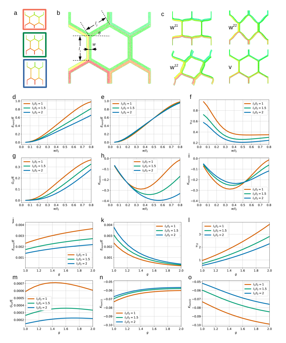
Refer to caption
Figure 1. Unit cell problem. a. ‘Unit cell’ examples: isotropic cell shape l1/l2=1l_{1}/l_{2}=1 (red box), elongated cell shape l1/l2=1.5l_{1}/l_{2}=1.5 (green box) and l1/l2=2l_{1}/l_{2}=2 (blue box) with w/l2=0.05w/l_{2}=0.05 and θ=30\theta=30 for all. The color of the box corresponds to the color of lines in other graphs. b. Geometry of the ‘unit cell’ and definition of the geometrical parameters l1l_{1}, l2l_{2}, ww and θ\theta; c. Deformed ‘unit cell’ geometries corresponding to the four elementary solutions of the ‘unit cell’ problems (parameters E=1E=1, ν=0.35\nu=0.35, l1=1l_{1}=1, l2=1l_{2}=1, w=0.1w=0.1, θ=30\theta=30, 𝐅g=𝐈{\bf F}_{g}={\bf I}); d-i. Dependence of homogenized material properties on the relative wall thickness (no growth). All moduli are normalized by the cell wall Young modulus EE and are shown as a function of relative wall thickness w/l2w/l_{2}. d. Modulus along axis 1, Eh​o​m​1E_{hom1}; e. Modulus along axis 2, Eh​o​m​2E_{hom2}; f. First Poisson’s ration ν12\nu_{12}; g. Shear modulus, G12G_{12}; h-i. Diagonal elements of the effective material property KhomK_{\rm hom}. The off-diagonal elements vanish. j-o. Dependence of homogenized material properties on the degree of anisotropic growth. We consider here only growth along axis 1, with corresponding eigenvalue gg. All moduli are normalized by the cell wall Young modulus EE and are shown as a function of gg. The relative wall thickness is set to w/l2=0.05w/l_{2}=0.05. j. Modulus along axis 1, Eh​o​m​1E_{hom1}; k. Modulus along axis 2, Eh​o​m​2E_{hom2}; l. First Poisson’s ration ν12\nu_{12}; m. Shear modulus, G12G_{12}; n-o. Diagonal elements of the effective material property KhomK_{\rm hom}. The off-diagonal elements vanish.

In the case of non-growing cellular solids, previous studies have computed numerically the homogenized elasticity tensor and compared their results to asymptotic expansions and experimental results, see e.g. [34]. We validated our results by quantitatively comparing the dependence of the effective material properties embedded in 𝔼hom\mathbb{E}_{\rm hom} with the results presented in [34]. Qualitatively, a ‘unit cell’ in the form of a regular hexagon yields an isotropic homogenized medium, see Figure 1d-e. Elongating the unit cell in the x2x_{2}-direction only reduces the homogenized modulus in the x1x_{1}-direction. This is in agreement with the measurements on epidermal onion peels realized using a microextensometer setup [33]. The macroscopic (homogenized) Poisson’s ratio ν12\nu_{12} is comparatively large for thin walls and is reduced by elongating the unit cell in the x2x_{2}-direction, see Figure 1f. The shear modulus turns out to be particularly low for thin walls, and is lower for elongated cells than for regular hexagons, see Figure 1g. All homogenized properties converge to the microscopic properties when the empty space (cell inside) vanishes, i.e. w/l2→1w/l_{2}\to 1.

In our multiscale analysis we introduced a tensorial material property, KhomK_{\rm hom}, that accounts for the contribution of cell pressure to the macroscopic (homogenized) stress tensor. For the present choice of coordinate system (which corresponds to symmetry axes of the unit cell), KhomK_{\rm hom} is diagonal; the two diagonal elements of KhomK_{\rm hom} are shown in Figure 1h-i as functions of relative thickness. A regular hexagonal unit cell yields an isotropic KhomK_{\rm hom}, while an elongated hexagon an anisotropic KhomK_{\rm hom}, where the anisotropy increases with wall thickness (as it can be seen from the ratio Khom11/Khom22K_{\rm hom11}/K_{\rm hom22}).

In case of isotropic growth, neither 𝔼hom\mathbb{E}_{\rm hom} nor KhomK_{\rm hom} depends on the degree of the growth. In contrast, when growth is anisotropic, the effective material properties change with growth anisotropy. In order to illustrate this, we show in Figure 1j-o the macroscopic (homogenized) material properties as a function of the degree of growth gg, when there is only growth along axis 1, for a fixed relative wall thickness. The macroscopic (homogenized) Young’s modulus in growth direction increases with gg, see Figure 1j, while the perpendicular modulus decreases, see Figure 1k. Inversely, the absolute value of KhomK_{\rm hom} in growth direction decreases with gg, see Figure 1n, while the absolute value of the other element increases, see Figure 1o. The macroscopic (homogenized) Poisson’s ratio ν12\nu_{12} increases with gg. Finally, the macroscopic (homogenized) shear modulus is non-monotonic.

5.2. Validation and sensitivity analysis for tissues with homogeneous material properties

Refer to caption
Figure 2. The coupled simulation and its validation. a. The coupled simulation involves in parallel a fine mesh 𝔪\mathfrak{m} and a coarse mesh 𝔐\mathfrak{M} of the tissue; b. Simplified diagram of the coupled simulation algorithm, emphasising the usage of the two meshes; c. One-factor-at-a-time sensitivity of growth rate to model parameters around their reference values (E=1E=1, ν=0.3\nu=0.3, l1=l2=1l_{1}=l_{2}=1, w=0.05w=0.05, θ=30\theta=30, η=1\eta=1, τ=0\tau=0), for both stress-based and strain-based growth; d-f. Superimposition of the cellular (cell number, Nx=16N_{x}=16) and continuous representations of tissue at t=0t=0 (e) and at t=60t=60 using either strain-based (e) or stress-based (f) growth-law – the smaller shaded area in e-f indicates the initial tissue geometry; g-h. Relative error (difference between coupled simulations and full microscopic model) of the displacement components u1u_{1} and u2u_{2} as a function of the cell number NxN_{x}; i-j. Mean growth rate as a function of time, with strain-based (i) or stress-based (j) growth law. The coupled simulation is compared with the microscopic simulation for several values of cell number, NxN_{x}, and of wall thickness to length ratio, w/l2w/l_{2} – all but w/l2w/l_{2} parameters are the reference parameters.

In order to further validate the multiscale method and the macroscopic model derived from the microscopic description of the growth and elastic deformations, we first consider on the one hand a tissue of Nx2/2N_{x}^{2}/2, with Nx=16N_{x}=16, identical regular hexagonal cells with microscopic geometrical parameters the cell wall length 4​δ​l14\delta l_{1}, 4​δ​l24\delta l_{2}, the cell wall thickness 4​δ​w4\delta w, and the angle θ\theta, where δ=1/Nx=1/16\delta=1/N_{x}=1/16, l1=l2=1l_{1}=l_{2}=1, w=0.05w=0.05 and θ=π/3\theta=\pi/3, and on the other hand a continuous tissue of the same size. The cell wall material properties, E=1E=1 and ν=0.3\nu=0.3, and the pressure, P1=0.001P_{1}=0.001, are homogeneous over the tissue. In Figure 2d-f, we superimposed the initial states of the microscopic cellular structure and of the continuous tissue, and we visually find that the continuous tissue evolved with the macroscopic model corresponds well to the cellular tissue evolved with the microscopic model at t=60t=60, both for the strain- and the stress-based growth law, see Figure 2e-f.

We varied the number of cells by scaling their size while keeping tissue dimensions unchanged, and considered three values of relative wall thickness, w/l2=0.05w/l_{2}=0.05, 0.10.1 and 0.20.2. We analysed the relative error given by the relative difference of solutions obtained from the coupled macroscopic simulations and microscopic simulations, see (72) in Appendix. Figures 2g-h show the relative error of the displacement components u1u_{1} and u2u_{2} at the first time step as a function of the number of cells NxN_{x}. This relative error is higher for thinner walls and it decays with the number of cells. Accordingly, the values of the growth rate are in agreement between microscopic and coupled macroscopic simulations, see Figures 2i-j. The larger error for a tissue of cells with thin walls compared to the error for a tissue of cells with thick walls for the same number of cells relates to the fact that the tissue with thick cell walls has smaller voids and is closer in the approximation to the homogeneous tissue than the tissue with thin cell walls. The mean growth appears constant in time and space, with thinner walls growing faster. This analysis verifies that the coupled simulation scheme enables the efficient computation of the tissue-scale behavior for a given microscopic cellular geometry and cell wall material properties, and provides a good approximation to the microscopic description of the problem.

In order to better understand the effects of microscopic parameters on the macroscopic behavior we performed a one-factor-at-a-time sensitivity analysis around reference values. We assumed the tissue to be homogeneous and we computed the sensitivity of growth rate with respect to each parameter, as defined by equation (73) in Appendix, see Figure 2c. As could be expected, growth rate increases with pressure, P1P_{1}, and extensibility, η\eta, while it decreases with yield threshold, τ\tau. Growth rate is less sensitive to yield threshold then to pressure and extensibility. Concerning microscopic geometric parameters (cell size, l2l_{2}, and wall thickness, ww) growth is promoted by thinner walls if cell size is constant or by larger cells if wall thickness is constant.

Finally, we note a fundamental difference between the two growth models: while the strain-based growth rate decreases with cell wall Young modulus EE and Poisson ratio ν\nu, these microscopic material properties have no effect on the stress-based growth.

5.3. Validation and predictions based on the dynamics of tissues with heterogeneous material properties

Refer to caption
Figure 3. Validation and illustration with gradients of material/geometric properties. First column: One factor-at-a-time parameter scan around the reference model for the homogeneous macroscopic coupled simulation. The results for the reference parameter values are indicated by black dots. Second and third columns: Superimposition of the deformed reference tissues obtained from microscopic (excluding f and g) and from macroscopic coupled simulations, where all parameters are homogeneous, except for the parameter of focus in the row, which varies linearly with first coordinate (in initial geometry) between the minimum and maximum value of the xx-axis in first column.The shadowed area behind indicates the initial geometry of the tissue. In all simulations tm​a​x=60t_{max}=60, d​t=1dt=1; the number of cells is Nx=16N_{x}=16 for microscopic simulations. The second and third columns correspond to strain-based and stress-based growth hypotheses, respectively. The parameters varied in each row are: a. Cell-wall Young modulus, EE; b. Cell-wall Poisson ratio, ν\nu; c. Pressure, P1P_{1}; d. Strain/stress threshold value, τ\tau; e. Extensibility, η\eta; f. Wall thickness, ww; g. Cell size, l1=l2l_{1}=l_{2}.

Now we consider more complex configurations in which material or geometric properties vary spatially, and we use them to further validate the agreement of macroscopic coupled simulations with simulation results for the microscopic model.

Beforehand we perform a parameter scan on larger intervals in the context of homogeneous tissues, and we present in the first column of Figure 3 the growth rate as a function of the parameters for strain- and stress-based growth hypotheses, as predicted by the macroscopic model. The reference situation is highlighted by black dots on each graph. For several parameters the dependence is affine, so that the sensitivity analysis in Figure 2c, which was restricted to small variations around the reference values, already captured the essence of the behavior. We find a non-affine dependence of the growth rate on the cell wall Young modulus for strain based growth, and on cell wall thickness for both growth hypotheses. We also note that the results for the strain-based and stress-based growth rates are identical when the Poisson ratio is equal to zero and all other parameters take their reference values, providing an additional check of the numerical simulation codes.

As next, we consider spatial heterogeneity of each parameter one-by-one, where all other parameters are homogeneous and take the reference value. We consider linear variations of the parameter along the first axis of the tissue, spanning the same interval for which the growth rate variation was presented in the homogeneous context, see the first column of Figure 3. In the second and third columns of Figure 3 we present the superposition of the corresponding tissues at t=60t=60 for the strain-based and stress-based growth hypothesis, respectively. For the five parameters, EE, ν\nu, P1P_{1}, τ\tau, η\eta, there is a quantitative agreement of tissue shape and size between macroscopic coupled simulations and microscopic simulations. This outcome further validates the multiscale procedure in a context where an additional mechanical stress is induced by spatial differences in growth rate.

Finally, we note that implementing gradients of geometrical properties is not trivial in the microscopic model, whereas such gradients can be easily implemented in the macroscopic coupled simulations. In Figure 3f-g, we present initial and final tissue shape for gradients in thickness, ww, and cell size, l2l_{2}, as predicted by the macroscopic two-scale model.

6. Conclusions

We formulated a microscopic model for the growth of plant tissues and derived the corresponding macroscopic equations, when the limit of the ratio between cell size and tissue size δ\delta tends to zero. Both methods, the formal asymptotic expansion and rigorous two-scale convergence, are used to revise the macroscopic equations. Passing to the limit in the nonlinear equations, resulted from the multiplicative decomposition of the deformation gradient into elastic and growth parts, requires the strong convergence of {𝐅g,δ}\{{\bf F}_{{\rm g},\delta}\}, the proof of which was the main technical step in the analysis. To show the strong convergence for the sequence of solutions of the microscopic problem and uniqueness for the macroscopic problem we used assumptions on the boundedness of the deformation gradient, which may be shown using the regularity results for solutions of the linear elasticity equations. The multiscale analysis performed here will also apply to other multiscale models for the growth of biological tissues.

The macroscopic two-scale model comprises the coupled system of equations of linear elasticity for the displacement and nonlinear ordinary differential equations for the growth tensor, that are additionally coupled to the ‘unit cell’ problems describing cell-scale properties and behaviour. This approach notably enables mapping the parameters of microscopic models that account for cell level characteristics to those of the macroscopic models defined on the tissue level, helping to bridge two relatively separate worlds in current models of plant growth. We implemented both models (microscopic and macroscopic) numerically and compared them quantitatively. The macroscopic coupled model requires less computational time for its numerical solution and can be readily adapted to describe spatial variations of parameters. Future work will address more complex spatial patterns of properties, such as accounting for variations in material properties across the cell wall, or additional physics, such as feedback from stress on material properties or hydraulics of water movement during growth. More generally, homogenization and the corresponding multiscale models appear as promising approaches to quantitatively describe morphogenesis.

Appendix A Components of the elastic tensor

The elasticity tensor in two dimensions is implemented as a six-component structure, where every component varies spatially,

𝔼={E0,E1,E2,E3,E4,E5}={E1111,E2222,E1122,E1212,E1112,E2212}.\begin{array}[]{llllllll}\mathbb{E}&=&\{E_{0},&E_{1},&E_{2},&E_{3},&E_{4},&E_{5}\}\\ &=&\{E_{1111},&E_{2222},&E_{1122},&E_{1212},&E_{1112},&E_{2212}\}\textrm{.}\end{array}

For an isotropic material in 2 dimensions, or in 3 dimensions with plane stress conditions, the components of the elasticity tensor using Lamé’s parameters λ\lambda and μ\mu are given by

𝔼={2​μ+λ,2​μ+λ,λ,μ,0,0}, with ​μ=E2​(1+ν),λ=E​ν1−ν2,\mathbb{E}=\{2\mu+\lambda,2\mu+\lambda,\lambda,\mu,0,0\},\quad\text{ with }\;\;\mu\ =\ \frac{E}{2(1+\nu)},\quad\lambda\ =\ \frac{E\nu}{1-\nu^{2}},

where EE and ν\nu are Young’s modulus and Poisson’s ratio respectively.

Given an elasticity tensor 𝔼\mathbb{E} in 2 spatial dimensions, for an orthotropic material with symmetry axes along the two Cartesian axes (E1112=E2221=0E_{1112}=E_{2221}=0), its material properties, such as the Young moduli E1E_{1} and E2E_{2} in the symmetry directions as well as the Poisson ratio ν12\nu_{12} and shear modulus G12G_{12}, can be computed as

E1=E1111−E11222E2222,E2=E2222−E11222E1111,ν12=E1122E2222,G12=E1212.E_{1}\ =\ E_{1111}-\frac{E_{1122}^{2}}{E_{2222}},\quad\quad E_{2}\ =\ E_{2222}-\frac{E_{1122}^{2}}{E_{1111}},\quad\quad\nu_{12}\ =\ \frac{E_{1122}}{E_{2222}},\quad\quad G_{12}\ =\ E_{1212}.

Appendix B Error and sensitivity definitions

For the quantity aδa^{\delta} defined in the microscopic domain (tissue) Ωδ\Omega^{\delta} and its corresponding macroscopic quantity AA defined in the macroscopic domain (tissue) Ω\Omega, we define the relative error eδe^{\delta} as

(72) eδ​(aδ,A)=∫Ωδ(aδ−A)2​𝑑x∫ΩδA2​𝑑x.e^{\delta}(a^{\delta},A)=\sqrt{\frac{\int_{\Omega^{\delta}}(a^{\delta}-A)^{2}dx}{\int_{\Omega^{\delta}}A^{2}dx}}.

The sensitivity ϕ⁡(X,x)\phi(X,x) around the reference model of an output quantity XX to the value of parameter xx is defined as

(73) ϕ⁡(X,x)=x0X⁡(x0)​∂X∂x|x=x0,\phi(X,x)=\frac{x_{0}}{X(x_{0})}\frac{\partial X}{\partial x}\Big|_{x=x_{0}},

where x0x_{0} is the reference value of the input parameter xx and X⁡(x0)X(x_{0}) is the output value in the reference model (all input parameters are equal to their reference value). The sensitivities ϕ\phi are normalized, non-dimensional quantities, and thus sensitivities of the output to different input parameters can be compared.

Appendix C Two-scale convergence and periodic unfolding operator

We recall the definition and some properties of the two-scale convergence and periodic unfolding operator.

Definition C.1 (Two-scale convergence).

[3, 41] A sequence {uδ}\{u^{\delta}\} in Lp​(Ω)L^{p}(\Omega), with 1<p<∞1<p<\infty, is two-scale convergent to u∈Lp​(Ω×Y)u\in L^{p}(\Omega\times Y) if for any ϕ∈Lq​(Ω,Cper​(Y))\phi\in L^{q}(\Omega;C_{\rm per}(Y)), with 1/p+1/q=11/p+1/q=1,

limδ→0∫Ωuδ​(x)​ϕ​(x,x/δ)​𝑑x=1|Y|​∫Ω×Yu⁡(x,y)​ϕ​(x,y)​𝑑y​𝑑x.\lim_{\delta\to 0}\int_{\Omega}u^{\delta}(x)\phi\big(x,x/\delta\big)dx=\frac{1}{|Y|}\int_{\Omega\times Y}u(x,y)\phi(x,y)dydx.
Theorem C.2.

[5, 40] Let {vδ}⊂L2​(Γδ)\{v^{\delta}\}\subset L^{2}(\Gamma^{\delta}) satisfy δ​‖vδ‖L2​(Γδ)2≤C\delta\|v^{\delta}\|^{2}_{L^{2}(\Gamma^{\delta})}\leq C, then there exists a two-scale limit v∈L2​(Ω,L2​(Γ))v\in L^{2}(\Omega;L^{2}(\Gamma)) such that, up to a subsequence, vδv^{\delta} two-scale converges to v∈L2​(Ω×Γ)v\in L^{2}(\Omega\times\Gamma) in the sense that

limδ→0δ​∫Γδvδ​(x)​ϕ​(x,x/δ)​d​γδ=1|Y|​∫Ω×Γv⁡(x,y)​ϕ​(x,y)​d​γy​𝑑x, for any ​ϕ∈C0​(Ω,Cper​(Y)).\lim_{\delta\to 0}\delta\int_{\Gamma^{\delta}}v^{\delta}(x)\phi\big(x,x/\delta\big)d\gamma^{\delta}=\frac{1}{|Y|}\int_{\Omega\times\Gamma}v(x,y)\phi(x,y)d\gamma_{y}dx,\quad\text{ for any }\phi\in C_{0}(\Omega;C_{\rm per}(Y)).
Lemma C.3.

(i)  If {uδ}\{u^{\delta}\} is bounded in L2​(Ω)L^{2}(\Omega), there exists a subsequence (not relabelled) such that uδ⇀uu^{\delta}\rightharpoonup u two-scale as δ→0\delta\to 0 for some function u∈L2​(Ω×Y)u\in L^{2}(\Omega\times Y).

(ii)   If uδ⇀uu^{\delta}\rightharpoonup u weakly in H1​(Ω)H^{1}(\Omega) then uδ⇀uu^{\delta}\rightharpoonup u and ∇uδ⇀∇u+∇yu1\nabla u^{\delta}\rightharpoonup\nabla u+\nabla_{y}u_{1} two-scale, where u1∈L2​(Ω,Hper1​(Y)/ℝ)u_{1}\in L^{2}(\Omega;H^{1}_{\rm per}(Y)/\mathbb{R}).

To define the periodic unfolding operator, let [z]Y[z]_{Y} for any z∈ℝdz\in\mathbb{R}^{d} denote the unique combination ∑i=1dki​bi\sum_{i=1}^{d}k_{i}b_{i} with k∈ℤdk\in\mathbb{Z}^{d}, such that z−[z]Y∈Yz-[z]_{Y}\in Y, see e.g. [11, 13]

Definition C.4.

Let p∈[1,∞]p\in[1,\infty] and ϕ∈Lp​(Ω)\phi\in L^{p}(\Omega). The unfolding operator 𝒯δ\mathcal{T}^{\delta} is defined by

𝒯δ​(ϕ)​(x,y)={ϕ⁡(δ​[x/δ]Y+δ​y)for a.e. ​(x,y)∈(Ω∖Λδ)×Y,0for a.e. x∈Λδ,y∈Y, and ​𝒯δ​(ϕ)∈Lp​(Ω×Y).\mathcal{T}^{\delta}(\phi)(x,y)=\begin{cases}\phi\big(\delta\big[x/\delta\big]_{Y}+\delta y\big)\quad&\text{for a.e. }(x,y)\in(\Omega\setminus\Lambda_{\delta})\times Y,\\ 0&\text{for a.e. }x\in\Lambda_{\delta},\;y\in Y,\end{cases}\quad\text{ and }\;\mathcal{T}^{\delta}(\phi)\in L^{p}(\Omega\times Y).

For ψ∈Lp​(Γδ)\psi\in L^{p}(\Gamma^{\delta}) the boundary unfolding operator 𝒯Γδ\mathcal{T}^{\delta}_{\Gamma} is defined by

𝒯Γδ​(ψ)​(x,y)={ψ⁡(δ​[x/δ]Y+δ​y)for a.e. ​(x,y)∈(Ω∖Λδ)×Γ,0for a.e. x∈Λδ,y∈Γ, and ​𝒯Γδ​(ψ)∈Lp​(Ω×Γ).\mathcal{T}^{\delta}_{\Gamma}(\psi)(x,y)=\begin{cases}\psi\big(\delta\big[x/\delta\big]_{Y}+\delta y\big)\quad&\text{for a.e. }(x,y)\in(\Omega\setminus\Lambda_{\delta})\times\Gamma,\\ 0&\text{for a.e. }x\in\Lambda_{\delta},\;y\in\Gamma,\end{cases}\quad\text{ and }\;\mathcal{T}^{\delta}_{\Gamma}(\psi)\in L^{p}(\Omega\times\Gamma).

For ψ∈Lp​(Ωδ)\psi\in L^{p}(\Omega^{\delta}) the unfolding operator 𝒯Ywδ\mathcal{T}^{\delta}_{Y_{w}} is defined in (24).

Notice that in the main text we use the same notation 𝒯δ\mathcal{T}^{\delta} for all three types of unfolding operator.

Proposition C.5 ([12]).

Let {ψδ}\{\psi^{\delta}\} be a bounded sequence in Lp​(Ω)L^{p}(\Omega) for some 1<p<∞1<p<\infty. Then the following assertions are equivalent:
(i) {𝒯δ​(ψδ)}\{\mathcal{T}^{\delta}(\psi^{\delta})\} converges weakly to ψ\psi in Lp​(Ω×Y)L^{p}(\Omega\times Y); (ii) {ψδ}\{\psi^{\delta}\} converges two-scale to ψ\psi, ψ∈Lp​(Ω×Y)\psi\in L^{p}(\Omega\times Y).

We have the following properties of the periodic unfolding operator and the boundary unfolding operator:

(74) 𝒯δ(F(u,v))=F(𝒯δ(u),𝒯δ(v)),𝒯δ(v(t,x/δ))=v(t,y),x∈Ωδ,y∈Yw or y∈Γ,t∈(0,T),\displaystyle\mathcal{T}^{\delta}(F(u,v))=F(\mathcal{T}^{\delta}(u),\mathcal{T}^{\delta}(v)),\;\quad\mathcal{T}^{\delta}(v(t,x/\delta))=v(t,y),\;x\in\Omega^{\delta},y\in Y_{w}\text{ or }y\in\Gamma,\,t\in(0,T),
⟨𝒯δ​(v),𝒯δ​(u)⟩ΩT×Yw=|Y|​⟨v,u⟩ΩTδ−|Y|⟨v,u⟩Λδ,T,‖𝒯δ​(ϕ)‖Lp​(ΩT×Yw)≤|Y|1p​‖ϕ‖Lp​(ΩTδ),\displaystyle{\displaystyle\langle}\mathcal{T}^{\delta}(v),\mathcal{T}^{\delta}(u){\rangle}_{\Omega_{T}\times Y_{w}}=|Y|{\langle}v,u{\rangle}_{\Omega_{T}^{\delta}}-|Y|{\langle}v,u{\rangle}_{\Lambda_{\delta,T}},\;\;\quad\|\mathcal{T}^{\delta}(\phi)\|_{L^{p}(\Omega_{T}\times Y_{w})}\leq|Y|^{\frac{1}{p}}\|\phi\|_{L^{p}(\Omega_{T}^{\delta})},
‖𝒯δ​(ψ)‖Lp​(ΩT×Γ)≤δ1p​|Y|1p​‖ψ‖Lp​(ΓTδ)≤C⁡(‖ψ‖Lp​(ΩTδ)+δ​‖∇ψ‖Lp​(ΩTδ)),\displaystyle\|\mathcal{T}^{\delta}(\psi)\|_{L^{p}(\Omega_{T}\times\Gamma)}\leq\delta^{\frac{1}{p}}|Y|^{\frac{1}{p}}\|\psi\|_{L^{p}(\Gamma^{\delta}_{T})}\leq C\big(\|\psi\|_{L^{p}(\Omega^{\delta}_{T})}+\delta\|\nabla\psi\|_{L^{p}(\Omega^{\delta}_{T})}\big),

for u,v∈L2​((0,T)×Ωδ)u,v\in L^{2}((0,T)\times\Omega^{\delta}) or u,v∈L2​((0,T)×Γδ)u,v\in L^{2}((0,T)\times\Gamma^{\delta}), ϕ∈Lp​((0,T)×Ωδ)\phi\in L^{p}((0,T)\times\Omega^{\delta}), ψ∈Lp​(0,T,W1,p​(Ωδ))\psi\in L^{p}(0,T;W^{1,p}(\Omega^{\delta})) and FF is any linear or nonlinear function, see e.g. [12, 11, 13].

Lemma C.6 ([12]).

(i) If ϕ∈Lp​(Ω)\phi\in L^{p}(\Omega), then 𝒯δ​(ϕ)→ϕ\mathcal{T}^{\delta}(\phi)\to\phi strongly in Lp​(Ω×Y)L^{p}(\Omega\times Y), for 1≤p<∞1\leq p<\infty.

(ii) Let {ψδ}⊂Lp​(Ω)\{\psi^{\delta}\}\subset L^{p}(\Omega), with ψδ→ψ\psi^{\delta}\to\psi strongly in Lp​(Ω)L^{p}(\Omega), then 𝒯δ​(ψδ)→ψ\mathcal{T}^{\delta}(\psi^{\delta})\to\psi strongly in Lp​(Ω×Y)L^{p}(\Omega\times Y).

Numerical simulation codes

Numerical simulation codes for both microscopic model (8), (11) and macroscopic model (54), (55) can be found under https://gitlab.inria.fr/akiss1/planthom.

Acknowledgments

We would like to thank the Newton Institute of Mathematical Sciences (INI) and International Centre for Mathematical Sciences (ICMS) for organising the research programme ‘Growth, form and self-organisation’ and the workshop ‘Growth, form and self-organisation in living systems’ at which this work was started. We also acknowledge the support of the Centre Blaise Pascal’s IT test platform operated with SIDUS [48] at ENS de Lyon for the possibility to test our code on the center’s computers.

References

  • [1] S. Agmon, A. Douglis, and L. Nirenberg, Estimates near the boundary for solutions of elliptic partial differential equations satisfying general boundary conditions, i, Comm. Pure Appl. Math., 12 (1959), pp. 623–727.
  • [2] S. Agmon, A. Douglis, and L. Nirenberg, Estimates near the boundary for solutions of elliptic partial differential equations satisfying general boundary conditions, ii, Comm. Pure Appl. Math., 17 (1964), pp. 35–92.
  • [3] G. Allaire, Homogenization and two-scale convergence, SIAM Journal of Mathematics and Analysis, 23 (1992), pp. 1482–1518.
  • [4] G. Allaire, Shape Optimization by the Homogenization Method, Springer-Verlag New York, 2002.
  • [5] G. Allaire, A. Damlamian, and U. Hornung, Two-scale convergence on periodic surfaces and applications, in Proceedings of the International Conference on Mathematical Modelling of Flow Through Porous Media, A. Bourgeat, C. Carasso, and A. Mikelic, eds., World Scientific, Singapore, (1996), pp. 15–25.
  • [6] H. Alt, Linear Functional Analysis. An Application-Oriented Introduction, Springer, 2016.
  • [7] B. Bozorg, P. Krupinski, and H. Jönsson, Stress and strain provide positional and directional cues in development, PLOS Computational Biology, 10 (2014), p. e1003410.
  • [8] B. Bozorg, P. Krupinski, and H. Jönsson, A continuous growth model for plant tissue, Phys. Biol., 13 (2016), p. 065002.
  • [9] A. Cianchi and V. Mazya, Global boundedness of the gradient for a class of nonlinear elliptic systems, Arch. Rational Mech. Anal., 212 (2014), pp. 129–177.
  • [10] P. Ciarlet, Mathematical elasticity. Volume I: Three-dimensional elasticity, North-Holland, 1988.
  • [11] D. Cioranescu, A. Damlamian, P. Donato, G. Griso, and R. Zaki, The periodic unfolding method in domains with holes, SIAM Journal of Mathematics and Analysis, 44 (2012), pp. 718–760.
  • [12] D. Cioranescu, A. Damlamian, and G. Griso, The periodic unfolding method in homogenization, SIAM Journal of Mathematics and Analysis, 40 (2008), pp. 1585–1620.
  • [13] D. Cioranescu, A. Damlamian, and G. Griso, The Periodic Unfolding Method, Springer, 2019.
  • [14] D. Cioranescu and P. Donato, An Introduction to Homogenization, Oxford University Press, 1999.
  • [15] F. Corson, M. Adda-Bedia, and A. Boudaoud, In silico leaf venation networks: growth and reorganization driven by mechanical forces, Journal of Theoretical Biology, 259 (2009), pp. 440–448.
  • [16] E. Davoli, C. Gavioli, and V. Pagliari, A homogenization result in finite plasticity, arXiv::2204.09084v2, (2022).
  • [17] E. Davoli, K. Nik, and U. Stefanelli, Existence results for a morphoelastic model, J Appl Math Mech, (2022).
  • [18] G. Duvaut and J. Lions, Inequalities in Mechanics and Physics, Springer, 1976.
  • [19] R. Dyson, L. Band, and O. Jensen, A model of crosslink kinetics in the expanding plant cell wall: Yield stress and enzyme action, Journal of Theoretical Biology, 307C (2012), pp. 125–136.
  • [20] R. Dyson and O. Jensen, A fibre-reinforced fluid model of anisotropic plant cell growth, Journal of Fluid Mechanics, 655 (2010), pp. 472–503.
  • [21] L. Evans, Partial Differential Equations, AMS, 2010.
  • [22] A. Goriely, The Mathematics and Mechanics of Biological Growth, Springer, 2017.
  • [23] A. Goriely and M. B. Amar, On the definition and modeling of incremental, cumulative, and continuous growth laws in morphoelasticity, Biomechanics and Modeling in Mechanobiology, 6 (2007), pp. 289–296.
  • [24] O. Hamant, M. Heisler, H. Jönsson, P. Krupinski, M. Uyttewaal, P. Bokov, F. Corson, P. Sahlin, A. Boudaoud, E. Meyerowitz, Y. Couder, and J. Traas, Developmental patterning by mechanical signals in arabidopsis, Science, 322 (2008), pp. 1650–1655.
  • [25] F. Hecht, New development in FreeFem+⁣+++, J. Numer. Math., 20 (2012), pp. 251–265.
  • [26] N. Hervieux, M. Dumond, A. Sapala, A. Routier-Kierzkowska, D. Kierzkowski, A. Roeder, R. Smith, A. Boudaoud, and O. Hamant, A mechanical feedback restricts sepal growth and shape in arabidopsis, Current Biology, 26 (2016), pp. 1019–1028.
  • [27] U. Hornung and W. Jäger, Diffusion, convection, adsorption and reaction of chemicals in porous media, J. Differential Equations, 92 (1991), pp. 199–225.
  • [28] R. Huang, A. Becker, and I. Jones, A finite strain fibre-reinforced viscoelasto-viscoplastic model of plant cell wall growth, Journal of Engineering Mathematics, 95 (2015), pp. 121–154.
  • [29] V. V. Jikov, S. M. Kozlov, and O. A. Oleinik, Homogenization of Differential Operators and Integral Functionals, Springer–Verlag, 1994.
  • [30] C. Kenig, F. Lin, and Z. Shen, Homogenization of elliptic systems with Neumann boundary conditions, J Americal Math Society, 26 (2013), pp. 901–937.
  • [31] J. Khadka, J.-D. Julien, and K. Alim, Feedback from tissue mechanics self-organizes efficient outgrowth of plant organ, Biophysical J, 117 (2019), pp. 1995–2004.
  • [32] J. Lockhart, An analysis of irreversible plant cell elongation, Journal of Theoretical Biology, 8 (1965), pp. 264–275.
  • [33] M. Majda, N. Trozzi, G. Mosca, and R. Smith, How Cell Geometry and Cellular Patterning Influence Tissue Stiffness, International Journal of Molecular Sciences, 23 (2022), p. 5651,
  • [34] S. Malek and L. Gibson, Effective elastic properties of periodic hexagonal honeycombs, Mechanics of Materials, 91 (2015), pp. 226–240.
  • [35] R. M. H. Merks, M. Guravage, D. Inze, and G. T. S. Beemster, VirtualLeaf: an open-source framework for cell-based modeling of plant tissue growth and development, Plant Physiology, 155 (2011-02), pp. 656–666.
  • [36] A. Mielke and U. Stefanelli, Linearized plasticity is the evolutionary γ\gamma-limit of finite plasticity, J. Eur. Math. Soc., 15 (2013), pp. 923–948.
  • [37] J. Necˇ\check{\rm{c}}as, Direct Methods in the Theory of Elliptic Equations, Springer, 2012.
  • [38] P. Neff, On Korn’s first inequality with non-constant coefficients, Proc Royal Society of Edinburgh, 132A (2002), pp. 221–243.
  • [39] P. Neff, Local existence and uniqueness for quasistatic finite plasticity with grain boundary relaxation, Quarterly of Applied Mathematics, 63 (2005), pp. 88–116.
  • [40] M. Neuss-Radu, Some extensions of two-scale convergence, C. R. Math. Acad. Sci. Paris, 332 (1996), pp. 899–904.
  • [41] G. Nguetseng, A general convergence result for a functional related to the theory of homogenization, SIAM Journal of Mathematics and Analysis, 20 (1989), pp. 608–623.
  • [42] O. A. Oleinik, A. S. Shomaev, and G. A. Yosifian, Mathematical Problems in Elasticity and Homogenization, North-Holland, 1992.
  • [43] J. A. Oliveira, J. Pinho-da Cruz, and F. Teixeira-Dias, Asymptotic homogenisation in linear elasticity. Part II: Finite element procedures and multiscale applications, Computational Materials Science, 45 (2009), pp. 1081–1096.
  • [44] H. Oliveri, J. Traas, C. Godin, and O. Ali, Regulation of plant cell wall stiffness by mechanical stress: a mesoscale physical model, Journal of Mathematical Biology, 78 (2019), pp. 625–653.
  • [45] J. Pinho-da Cruz, J. A. Oliveira, and F. Teixeira-Dias, Asymptotic homogenisation in linear elasticity. Part I: Mathematical formulation and finite element modelling, Computational Materials Science, 45 (2009), pp. 1073–1080.
  • [46] W. Pompe, Korn’s first inequality with variable coefficients and its generalization, Comment. Math. Univ. Carolin, 44 (2003), pp. 57–70.
  • [47] M. Ptashnyk and B. Seguin, The impact of microfibril orientations on the biomechanics of plant cell walls and tissues: modelling and simulations, Bulletin of Mathematical Biology, 78 (2016), pp. 2135–2164.
  • [48] E. Quemener and M. Corvellec, SIDUS—the Solution for Extreme Deduplication of an Operating System, The LINUX Journal, January (2014).
  • [49] E. Rodriguez, A. Hoger, and A. McCulloch, Stress-dependent finite growth in soft elastic tissue, J Biomechanics, 27 (1994), pp. 455–467.
  • [50] E. Sanchez-Palencia, Non-homogeneous media and vibration theory, Springer-Verlag Berlin, 1980.
  • [51] Z. Shen, Boundary estimates in elliptic homogenization, Anal. PDE, 3 (2017), pp. 653–694.
  • [52] J. Simon, Compact sets in the space lp​(0,t,b)l^{p}(0,t;b), Annali di Matematica Pura ed Applicata volume, 146 (1986), pp. 65–96.
  • [53] E. Smithers, J. Luo, and R. Dyson, Mathematical principles and models of plant growth mechanics: from cell wall dynamics to tissue morphogenesis, Journal Of Experimental Botany, 70 (2019), pp. 3587–3600.
  • [54] R. Vandiver and A. Goriely, Tissue tension and axial growth of cylindrical structures in plants and elastic tissues, EPL (Europhysics Letters), 84 (2008), p. 58004.