On marginal feature attributions of tree-based modelsThanks: ∗Emerging Capabilities Research Group, Discover Financial Services Inc., Riverwoods, ILThanks: † first author, khashayarfilom@discover.comThanks: ‡ alexeymiroshnikov@discover.comThanks: § kostaskotsiopoulos@discover.comThanks: ¶ arjunravikannan@discover.com
Abstract.
Due to their power and ease of use, tree-based machine learning models, such as random forests and gradient-boosted tree ensembles, have become very popular. To interpret them, local feature attributions based on marginal expectations, e.g. marginal (interventional) Shapley, Owen or Banzhaf values, may be employed. Such methods are true to the model and implementation invariant, i.e. dependent only on the input-output function of the model. We contrast this with the popular TreeSHAP algorithm by presenting two (statistically similar) decision trees that compute the exact same function for which the “path-dependent” TreeSHAP yields different rankings of features, whereas the marginal Shapley values coincide. Furthermore, we discuss how the internal structure of tree-based models may be leveraged to help with computing their marginal feature attributions according to a linear game value. One important observation is that these are simple (piecewise-constant) functions with respect to a certain grid partition of the input space determined by the trained model. Another crucial observation, showcased by experiments with XGBoost, LightGBM and CatBoost libraries, is that only a portion of all features appears in a tree from the ensemble. Thus, the complexity of computing marginal Shapley (or Owen or Banzhaf) feature attributions may be reduced. This remains valid for a broader class of game values which we shall axiomatically characterize. A prime example is the case of CatBoost models where the trees are oblivious (symmetric) and the number of features in each of them is no larger than the depth. We exploit the symmetry to derive an explicit formula, with improved complexity and only in terms of the internal model parameters, for marginal Shapley (and Banzhaf and Owen) values of CatBoost models. This results in a fast, accurate algorithm for estimating these feature attributions.
1. Introduction
1.1. Motivation and summary of results
Ensemble methods combine a group of weak learners to produce a strong learner [16, 30]. In the context of tree-based models, examples of such an approach include random forests [7] and gradient-boosted tree ensembles [26]. Given their superior performance on structured data in various tasks [58, 9, 74, 31, 27, 64], tree-based models are frequently used in regulated domains such as financial services [14, 32] and healthcare
[71, 79].
Ensemble models are considered to be complex which raises concerns about their interpretability [59, 67], especially in view of regulations that require it, such as
the Equal Credit Opportunity Act (ECOA) and
the Fair Housing Act (FHA).
Financial institutions in the United States (US),
for instance, are required under the ECOA
to notify declined or negatively impacted applicants
of the main factors that led to the adverse action.
Determining the factor contributing the most to an outcome of a model may be done via individualized feature attributions.
An important approach to feature attribution is to utilize the celebrated work of Shapley [62] from cooperative game theory [65, 46].
To elaborate, consider the features (predictors) as random variables on a probability space . Given a model , one can define certain games with being the players. The machinery of the Shapley value [62] then allows us to quantify the contribution of each feature to a prediction of the model. Two of the most notable games in the literature are the marginal and conditional games,
which are defined respectively in terms of marginal expectations or
conditional expectations11
1
The expectations and are sometimes called interventional and observational expectations in the literature.
Other common notations are
or
for
, and
for .
(see [11])
| (1.1) |
Here, is an arbitrary point of , is a subset of , and (respectively ) denote the collections of ’s with (resp. ). Each or is a collection of functions , and hence they define -person games of the form for each . Thus, and are pointwise games. Shapley values provide a canonical way of assigning importance scores to ’s in any such game:
| (1.2) |
We call these feature attributions marginal and conditional Shapley values respectively. The former can be described as true to the model and are dependent on the structure of the model (thus better suited for explaining specific models), whereas the latter can be described as true to the data and take the joint distribution of features into account (hence they are much harder to compute) [11]. More generally, one can apply any linear game value to the games in (1.1) to obtain the corresponding marginal and conditional feature attributions. We will mainly consider game values of the form
| (1.3) |
which are generalizations of the Shapley value, and satisfy the desirable null-player property, i.e. they assign zero to players that do not contribute to any coalition. This results in the so-called missingness property of the corresponding explainers [46].
We shall exploit this property in our treatment of tree ensembles
to reduce the complexity of computing marginal feature attributions; compare with [8].
Game-theoretic feature attributions can be investigated from different angles:
the model in hand, the game chosen based on and the predictors, and the game value applied to it.
Let us motivate this:
- (i)
For tree-based models, is piecewise constant, i.e. a simple function in the measure-theoretic sense.
- (ii)
The conditional and marginal games from (1.1), and hence and , are dependent only on the input-output function , not on how is implemented or on any internal parameters such as weights of a neural network or proportions of splits of data points in a decision tree. When is obtained from a tree ensemble, we shall prove that the marginal game , and thus feature attributions obtained from a linear game value , are also simple functions; see Theorem 3.2. This is not the case for the conditional game as demonstrated in Example 3.1. Furthermore, for tree-based models, there is an empirical game (see Definition 2.8) where is an ensemble trained on a dataset. This is the game whose Shapley values are outputs of the path-dependent variant of the popular TreeSHAP algorithm [45, 44]. In Section 3.2, we shall show that this game does not estimate either the marginal or the conditional game, even for very big datasets. Moreover, we observe that the feature attributions generated by TreeSHAP fail to satisfy the desirable property of implementation invariance which is posed as an axiom in [69]. This is shown in Section 3.1, where for two topologically distinct decision tree regressors that exhibit identical input-output functions and even very close impurity measures, the most contributing features in terms of TreeSHAP turn out to be different over a non-negligible subset of data (cf. Figure 1). A similar example is presented for the “eject” variant of TreeSHAP ([8]) in Appendix C.2.
- (iii)
Game values other than Shapley appear in the literature too. One well-known example is the Banzhaf value [6]. In particular, it is suggested that to bridge the gap between the marginal and conditional frameworks one can group the features based on a dependence measure, and then either consider a quotient game, or utilize a coalitional game value, for example the Owen value [53] or the two-step Shapley value [37], that takes into account the provided partition of features [48, 1, 35] (see Appendix B.4 for another natural application of coalitional values). We advocate for the carrier-dependence property (and its coalitional analog) that, along with the null-player property, allows us to reduce the dimensionality of the problem of computing marginal feature attributions. See Appendix B for necessary background material from cooperative game theory, and Theorem 2.4 for a classification of game values with properties that we deem desirable when it comes to tree ensembles.
A key insight, alluded to above, is that the number of distinct features on which a tree from the ensemble splits is usually smaller than the total number of features; compare with experiments in Section 4.2.22
2
The number of features on which a learner depends can also be limited through hyperparameter tuning e.g.
the
max_feature
hyperparameter in scikit-learn’s bagging module or the
colsample_bytree
hyperparameter in XGBoost and LightGBM.
A feature absent from a tree is a null player for the corresponding marginal game (not valid for the conditional game; cf. Lemma 2.1).
So when a linear game value with null-player and carrier-dependence properties is used (e.g. Shapley, Banzhaf etc.), features not appearing in a tree do not get a contribution from it; and for the rest, the computations only involve features that do come up.
Therefore, the complexity of computing the value for the game becomes
where is the maximum number of features relevant to
a tree, and is the total number of trees in the ensemble .
The observation just made on the number of different features per tree is best demonstrated by
Explainable Boosting Machine (EBM) [52], where each tree is dependent on at most two features (see Example 3.3); and more importantly, by CatBoost models [21] where the trees are
oblivious (symmetric). Indeed, the number of distinct features appearing in such a tree does not exceed the depth which is rarely larger than .33
3
The recommended range of the hyper-parameter
depth
is to per CatBoost documentation https://catboost.ai/en/docs/concepts/parameter-tuning [17].
As a matter of fact, oblivious trees play a central role in this article:
-
In Section 3.4, we simplify the Shapley formula to obtain a formula of reduced complexity for the marginal Shapley values of a symmetric decision tree (or an ensemble of such objects) which is solely in terms of the internal parameters of the model and does not require any access to the training data; see Theorem 3.6.
-
We generalize the aforementioned explicit formula from the Shapley value to any other game value apt for explaining tree ensembles according to Theorem 2.4 (e.g. the Banzhaf value). It can also be generalized for a large family of coalitional game values (of which the Owen value is an example). See Appendix F for more details.
-
Our explicit formulas for marginal feature attributions of ensembles of oblivious trees can be thought of as an “intrinsic interpretability method” (see [36] for a taxonomy of Explainable AI) due to their reliance on internal model parameters rather than on any background dataset. The benefit of symmetry to interpretability showcased by such formulas is reminiscent of a general philosophy that intrinsic interpretability should be induced from certain constraints [76]. Examples of this approach include working with ReLU networks or with neural network architectures which implement functions of a special form [3, 72, 66, 77, 80], or papers [52, 63] on tree ensembles where the number of features per tree or the total number of splits across the ensemble are restricted. Nevertheless, unlike those articles, we work with game-theoretic local feature attributions. Furthermore, in our case, it is well documented that tree ensembles can have competitive predictive power even with the symmetry constraint [24, 29].
-
Estimating marginal Shapley values based on a background dataset, i.e. considering the empirical marginal game (cf. (2.2)), can be subtle: The background dataset should be large for the sake of statistical accuracy because the mean squared error of such estimators is typically inversely proportional to the size of the background dataset (see Lemma D.3); but the complexity increases with the size of the background dataset—this last point is especially manifested for the interventional TreeSHAP algorithm [44]. Building on Theorem 3.6, we present Algorithm 3.12 for oblivious ensembles that alleviates this problem of reliance on a background dataset, and computes the exact Shapley values of the empirical marginal game based on the whole training set. We carry out a rigorous error analysis for this algorithm in Theorem 3.15. Table 1 below summarizes all of these facts by comparing our method with TreeSHAP in terms of accuracy and complexity.
| Algorithm | Precomputation complexity (per leaf) | Computation complexity (for an input explicand) | Variance of error is governed by |
| Path-dependent TreeSHAP [45] | N/A | N/A | |
| Interventional TreeSHAP [44] | N/A | ||
| Algorithm 3.12 |
It must be pointed out that results of Section 3.4 can yield an analytic formula for the marginal Shapley values of any decision tree, even if they are not symmetric (e.g. those constructed by LightGBM [39] or by XGBoost [13]): from any given decision tree , one can construct an oblivious decision tree computing the exact same function (cf. Figure 9) to which Theorem 3.6 can then be applied to obtain an explicit formula for the marginal Shapley values. Nevertheless, in the absence of symmetry, determines a finer partition of the domain whose associated probabilities cannot always be estimated based on the trained tree . These probabilities appear in the formula, and can in principle be precomputed using a background dataset. We elaborate more on the case of non-oblivious trees in Appendix G. Finally, we point out that the rectangularity of regions cut by decision trees is crucial to our results. In fact, it is observed in Appendix H that, in case of ReLU networks, marginal Shapley values are much more complicated as piecewise functions with respect to the activation regions.
1.2. Outline
Section 2 is devoted to the necessary background material including a very brief review of machine learning explainability and a short discussion on different boosting libraries along with the TreeSHAP method for interpreting them. We present our main results in Section 3: In Section 3.2, we show that for tree-based models feature attributions arising from either TreeSHAP or the marginal game are simple functions. However, the former can depend on the model’s make-up, and hence are not implementation invariant; see Section 3.1. Next, focusing on marginal feature attributions, in Section 3.3 we observe that, for computing the marginal contribution of a feature, only the subset of trees which split on that feature are relevant; and each of those trees often depends only on a portion of the variables. This observation, showcased through experiments with XGBoost, LightGBM and CatBoost models in Section 4.2, can be utilized to reduce the complexity of computing marginal feature attributions for tree ensembles. The most important example is the case of CatBoost models where, leveraging the symmetry of oblivious trees, in Section 3.4, we obtain an explicit formula for marginal Shapley values as simple functions, and we propose an algorithm based on that. The relevant experiments appear in Sections 4.3 and 4.1. See Appendix A for code and data availability.
2. Preliminaries
2.1. Basic conventions and notation
- •
For random variables, upper-case letters are used; and vector quantities are written in bold font.
- •
In this article, always is a finite non-vacuous subset of positive integers whose cardinality is denoted by . Except in the appendices, is taken to unless stated otherwise.
- •
For an -dimensional vector and a subset of indices, we use as a subscript to show the vector formed by components whose indices come from . For instance, if , then . Moreover, is denoted by ; thus one may write as .
- •
In modeling problems, the features are denoted by a vector of random variables on an ambient probability space . The joint probability distribution is the Borel probability measure on obtained from the pushforward of the probability measure on . The model is thought of as a Borel measurable function . We use to denote a finite data sample. Occasionally, a smaller background dataset may be required for estimating marginal expectations; that will be denoted by . A random sample drawn i.i.d. from according to the distribution is shown by whose elements are random vectors
These are i.i.d. and for each of them the induced measure on is .
- •
We assume that the features have numeric value; so they can be continuous, ordinal or encoded categorical features. (See Appendix B.4 for more on the case of categorical features.) We assume that each takes its values in an interval . Thus is supported in the hypercube
(2.1)
2.2. A review of machine learning explainability
There is a vast literature on explaining complicated machine learning models;
see [49, 36] for an overview.
There are global methods such as PDP (Partial Dependence Plots) [26]
or BETA (Black Box Explanations through Transparent Approximations) [42]
which describe the overall effect of features as well as local methods such as
the rule-based method Anchors [57], or
LIME (Linear Interpretable Model-agnostic Explanation) [56]
and SHAP (SHapley Additive exPlanations) [46]
which provide individualized feature attributions to explain a single prediction.
The SHAP paper builds on ideas from game theory [62]
(also see [65]).
Moreover, it introduces the KernelSHAP algorithm for approximating Shapley values.
For a survey on different methods for estimating Shapley values,
see [10].
This paper focuses on game-theoretic local feature attributions.
All the aforementioned methods are model agnostic.
There are also model-specific methods for estimating Shapley values including
the DeepSHAP algorithm for neural networks [12], and the TreeSHAP algorithm
[45, 44] for tree ensembles.
The focus of this paper is on tree-based models.
After a brief review of TreeSHAP in Section 2.5,
we compare its outputs with marginal feature attributions in Section 3 where we expose certain shortcomings of TreeSHAP, and discuss how calculating marginal feature attributions for tree-based models can be done more efficiently.
2.3. Feature attributions via cooperative game theory
Machine learning explainers studied in this paper are constructed via game-theoretic methods.
The first step is to define certain pointwise games based on the predictors and the model . At each point , these define a game with as its set of players, i.e. a set function . Next, to compute feature attributions for the individual , a game value is applied to
obtain a vector where the component quantifies the “contribution” of player (feature ) according to . We refer the reader to Appendix B for basic notions from cooperative game theory.
Two prominent games associated with a machine learning model are the marginal game and the conditional game defined in (1.1).
Feature attributions obtained from them via applying a game value such as Shapley are characterized as true to the model and true to the data respectively; this is best demonstrated in Example B.7.
In general, the choice between the two approaches depends on the application [11].
See [48] for a detailed comparison of marginal and conditional feature attributions.
It is certainly possible to define other games based on the model ; see [15, 47, 68]. Another game particularly important to our context is the game that the path-dependent TreeSHAP algorithm ([45]) introduces when
is computed by a trained tree ensemble ; cf. Section 2.5.
The resulting feature attributions turn out to be very different from either marginal or conditional ones as we shall observe in Section 3.1.
It should be mentioned that in our treatment conditional and marginal games stem from features that are random variables defined on an ambient probability space. There is also the empirical marginal game which is an estimator for the marginal game based on the training set (or based on any other data sample):
| (2.2) |
An important observation, which is useful for reducing the computational complexity of generating marginal feature attributions, is that for the marginal game only variables that do appear in the model matter. This is not the case for the conditional game.
Lemma 2.1.
Consider where are the predictors and is a function.
- (1)
If and is independent of for , then for -almost every , each is a null player of the game and is a carrier for it. Moreover, can be considered as a function of lower arity: where is defined by .
- (2)
Suppose and is independent of for . If is independent of , then is a null player of the game for -almost every . Furthermore, if is independent of , then is a carrier of for -almost every .
We refer the reader to Appendix B.1 for basic concepts from game theory such as null player or carrier. The lemma above is proven in Appendix B.2. Notice that, here, in the case of the marginal game, one can focus on games with a smaller set of players instead of whereas additional assumptions on predictors’ joint distribution are required when it comes to the conditional game.
Remark 2.2.
Next, we discuss how certain properties of game values can be desirable in constructing machine learning explainers. Various properties of game values have been studied extensively in the game theory literature. The seminal paper of Shapley [62] shows that the Shapley value
| (2.3) |
is the unique game value with linearity, symmetry, efficiency and null-player properties.44 4 In fact, Shapley’s theorem holds with the weaker property of additivity in place of linearity. Moreover, his paper combines efficiency and null-player properties into a single formula. Another characterization of the Shapley value is due to Young; it drops additivity and replaces the null-player property with strong monotonicity [78]. Formal definitions of these properties can be found in Appendix B.1. For our purposes, as mentioned in Section 1.1, the null-player property is crucial. It turns out that linear game values with the null-player property are precisely those of form (1.3). Indeed, it is possible to determine when game values of this form satisfy other desirable properties just mentioned; this is the content of Lemma B.2. The lemma allows us to deal with a formula of the form (1.3) (or (B.4)) rather than an abstract assignment , a formula in which games associated with a machine learning model (e.g. (1.1)) can be plugged. Notice that the Shapley value (2.3) is of the form (1.3). The same holds for the famous Banzhaf value (cf. [6])
| (2.4) |
Lemma B.2 immediately implies that both Shapley and Banzhaf game values are linear, symmetric, strongly monotonic, and satisfy the null-player property.55 5 Nonetheless, among them, only the Shapley value satisfies the efficiency property due to the main result of [62]. Moreover, they satisfy the carrier dependence property; see Lemma B.10.66 6 For the carrier dependence of the Shapley value, also see [62, Corollary 2]. Notice that, due to the symmetry, the weights in (2.3) and (2.4) depend only on the and . Thus the formulas make sense even when the set of players is an arbitrary finite subset of in bijection with . When and the context is clear, we omit and write these values as or .
Example 2.3.
For a game with the set of players one has
| (2.5) |
Different properties of game values mentioned so far have come up in the context of machine learning explainability. Paper [46] puts forward the SHAP framework for individualized feature attribution which is argued to be the unique additive method satisfying missingness and consistency. These properties of the SHAP method follow respectively from efficiency, null-player and strong monotonicity properties of the Shapley game value. Paper [68] discusses why different properties of the Shapley value are desirable and construct explainers by applying the Shapley value to a variety of games constructed based on the model in hand. In our setting of marginal explanations for tree ensembles, as mentioned in Section 1.1, the key insight, best demonstrated by libraries such as EBM and CatBoost, is that the number of distinct features appearing in a tree can be much smaller than the total number of variables. In view of this, we postulate that game values used for explaining tree ensembles should admit the following properties (see Definition B.1):
- (1)
linearity, so that feature attributions can be disaggregated across the ensemble;
- (2)
symmetry, a natural property which is often assumed in the literature;
- (3)
null-player, so that features on which a tree does not split get zero attributions from that tree;
- (4)
carrier-dependence, so that for each tree the problem reduces to one only involving the features on which the tree actually splits.
The advantage of the null-player property has been pointed out in [8] as well. But in this article, we formulate a unified framework by considering game values satisfying the four axioms above which include game values other than Shapley, e.g. Banzhaf. The theorem below completely classifies such game values.
Theorem 2.4.
Let be a collection of real numbers with a “backward” Pascal identity:
| (2.6) |
Define a game value by setting
| (2.7) |
for any cooperative game and any . Then satisfies linearity, symmetry, null-player and carrier-dependence axioms. Conversely, a game value satisfying these four axioms is of the form for such a collection .
A proof will be presented in Appendix E.1. Moreover, such game values have a computational advantage because certain sums involving their coefficients may be simplified; this is the content of Lemma E.1.
Example 2.5.
In the case of the Shapley value one has while in the case of the Banzhaf value. It can be readily checked that the backward Pascal identity (2.6) holds in both situations.
At the end of this section, we allude to coalitional explainers. On the game-theoretic side, they amounts to adding a coalition structure (cf. [5]) and then applying a coalitional game value; i.e. an assignment where is a partition of the set of players . This pertains to machine learning explanation because it has been observed that grouping predictors can improve the stability of feature attributions and facilitate computations [48, 1, 35]. One well-known example of a coalitional game value is the Owen value introduced in [53]:
| (2.8) |
We shall discuss coalitional game values in more details in Appendix B.3. Many of our results can be generalized from game values such as Shapley or Banzhaf to coalitional game values such as Owen. In particular, a coalitional version of Theorem 2.4 is presented in Appendix E.2. Furthermore, we shall see in Appendix B.4 that the Owen game value can be used naturally to retrieve marginal Shapley values of categorical features which were one-hot encoded in the modeling process. For more on group explainers, including a detailed treatment of various axioms for coalitional game values and their implications, see [48].
2.4. Tree ensembles
We start with some basic notation and terminology.
- •
We are mainly concerned with tree-based regressors. Such a model corresponds to an ensemble where ’s are regression decision trees. We always assume that the ensembles are trained, so provides us with the knowledge of internal parameters such as values at the leaves and the splitting proportions of training instances at the internal nodes of trees. Denoting the function implemented by as , one has . For classifiers, outputs of ’s become logit probability values and becomes the decision function (the population minimizer).77 7 The function can be accessed by setting prediction_type="RawFormulaVal" in CatBoost and raw_score=True in LightGBM. Moreover, sometimes is an affine transformation of .
- •
In each decision tree from the ensemble, splits at non-terminal nodes are based on whether a feature is smaller than a threshold or not. To avoid ambiguity about if should be strict or not, we assume all events are of probability zero.88 8 Ordinal features fit in this framework too. For instance, if takes its values in , one can take the threshold to be a non-integer from . In other words:
(2.9) - •
For each , the subset of trees in that split on is denoted by .
- •
Each decision tree from ensemble computes a simple function
(2.10) where are the values appearing at the leaves of and are the rectangular regions with disjoint interiors determined by it; here is the region where the tree assigns the value and its characteristic function is denoted by . Therefore, the ambient hypercube (2.1) is cut into smaller ones which are determined by the splits in the decision tree. We take these hypercubes to be closed. They then may intersect each other along the boundaries, but that is negligible in view of (2.9). Thus
(2.11) is a partition of into smaller hypercubes, at least in the measure-theoretic sense.99 9 I.e. the union of covers except for perhaps a measure zero subset, and the intersection of any two of them is of measure zero.
- •
Any partition of into rectangular regions may be completed into a grid which is the product of partitions determined by across different dimensions. Figure 2 illustrates a decision tree computing a simple function of two variables along with the corresponding partition and the finer one .
Various implementations of gradient boosting differ in terms of the training time, their hyperparameters, their optimization and regularization techniques, their approach to construct trees, their handling of categorical features or missing values, parallel processing etc. For instance, the implementation of gradient boosting in Scikit-learn uses gradient descent for minimizing the cost function while XGBoost utilizes the Newton method; or CatBoost has a sophisticated way of handling categorical features which XGBoost lacks. Regardless of implementation differences, when the base learner is a decision tree, ensembles obtained from bagging or boosting represent simple functions. The relevant point here is how trees constructed by different libraries are different topologically. The reader can check detailed comparisons of XGBoost, LightGBM and CatBoost methods in [61, 34, 51, 2]. Focusing on their (default) growth policy:
- •
Trees in XGBoost are constructed level-wise; they are grown to max_depth and are pruned based on hyperparameters such as min_split_loss [20]. The splits within a level are not necessarily the same.
- •
Trees in LightGBM are constructed in a leaf-wise manner; tree complexity is governed by hyperparameters such as max_depth and num_leaves [18]. This can result in asymmetric trees.
- •
Trees in CatBoost are symmetric or oblivious; this restriction can be thought of as a regularization helping to avoid overfitting [21]. See below for a definition of oblivious decision trees.
Definition 2.6.
An oblivious (symmetric) decision tree is a perfect binary tree (i.e. ) in which the splits across each level are done with respect to the same feature and threshold.
2.5. TreeSHAP algorithm and its variants
Although there are numerous algorithms for computing global feature importance values for a tree-based model, local feature attribution methods are not fully investigated [44, Supplementary Results, Section 2].
The TreeSHAP algorithm is one of the most common local methods for interpreting tree-based models.
TreeSHAP is not model agnostic and takes internal parameters such as values at the leaves and the splitting proportions at internal nodes into account. The algorithm has two variants which both use dynamic programming to obtain polynomial-time performance.
The original TreeSHAP algorithm [45], the path-dependent variant,
is meant to estimate conditional Shapley values; but its approach to approximating conditional expectations turns out to be imperfect [10, p. 18].
Indeed, the Shapley values generated by the path-dependent TreeSHAP come from a certain game associated with the trained ensemble [45, Algorithm 1]. This game is presented in Definition 2.8 below. In Section 3, we shall observe that this game differs from both conditional and marginal games, and as a matter of fact, it depends on the tree structure, not just the input-output function of the model.
In contrast, the other variant, the interventional TreeSHAP,
estimates marginal Shapley values through utilizing a background dataset [44]; it thus depends only on the input-output function of the model.
The downside is that a fair number of background samples is required for the accuracy of the estimation while the algorithm becomes slow for even moderately large background datasets (see the complexity analysis below). Indeed, experiments in the aforementioned paper use only background samples
[44, p. 66].
According to TreeSHAP documentation [19], the recommended size for the background dataset is between and .
In Section 3.4, we resolve this issue in the case of oblivious ensembles by presenting a method for estimating marginal Shapley values which does not require any background dataset and instead, employs
internal parameters; the accuracy of our method is dictated by the size of the training dataset.
In implementing TreeSHAP, the variant is determined by the hyperparameter
feature_perturbation
which should be
"tree_path_dependent"
for path-dependent, and
"interventional"
for the interventional variant—which is currently the default [19].
For an ensemble , the time complexity of the path-dependent TreeSHAP is
| (2.12) |
while that of the interventional one is
| (2.13) |
see [44, pp. 64–66] for descriptions of these algorithms and their complexity analysis.
Definition 2.8.
Let be a trained ensemble of decision trees and the features. Denoting the training set with the response values removed by , following our convention in Section 2.4, information such as leaf scores or members of that end up at a given node can be read off from . We define the associated TreeSHAP game as where, for decision trees, games are defined recursively in the following manner. In case that has no splits (so is a single leaf), assigns the value at the unique leaf of to every subset of . Next, suppose the split at the root of takes place with respect to feature and threshold . Thus we have the left subtree and the right subtree along with smaller datasets and . Then set
| (2.14) |
Note that is a carrier for each ; and
where is the function computed by the decision tree , and is the leaf value at .
It is not hard to show that the TreeSHAP game becomes the empirical marginal game (see (2.2)) if the predictors are independent. But the games are different in general; compare with [4].
We finish the section by pointing out the related algorithms which mostly build upon the original TreeSHAP method [45]. Paper [75] introduces “Fast TreeSHAP” as an improvement of the path-dependent TreeSHAP while [38] discusses an improvement when the Banzhaf value is used in place of Shapley.
Another approach is the unpublished work of Saabas [60] (cf. [44, Supplementary Results, Section 3]) where only features appearing along the decision path can get non-zero attributions.1010
10
Just like the path-dependent TreeSHAP, Saabas’ method also fails the implementation invariance.
Finally, [8] introduces a modified version of from (2.14) where, instead of taking a weighted average, one “ejects” the decision tree if the split is done with respect to a feature absent from . This game is presented in Definition C.1 of Appendix C.2. The authors then write the Shapley formula for this new game and simplify it to reduce the complexity. Nevertheless, as shown in the appendix, this approach also lacks implementation invariance, just like the original path-dependent TreeSHAP.
3. Main results
3.1. TreeSHAP is not implementation invariant
When two models are functionally equivalent, namely, they generate equal outputs for the same input, it is reasonable to ask for their associated feature attributions to coincide. This is the implementation invariance axiom for attribution methods which is set forth in [69]. Indeed, if this property holds, one can treat feature attributions as well-defined operators on some appropriate space of models. This has been carried out for conditional and marginal feature attributions in [48] where the resulting operators are thoroughly studied via tools from functional analysis. The goal of this section is to show that, unlike conditional and marginal frameworks, the path-dependent TreeSHAP fails this axiom and can depend on the model’s make-up.
Example 3.1.

Consider a simple regression problem with two predictors that are supported in the square , and the response variable which takes value in . We assume that is captured by the function where
are subrectangles inside .
Following our convention in Section 2.4, we assume that events and are of probability zero.
Therefore, the pushforward probability measure on is supported in ; and , and provide a measure-theoretic partition of .
The ground truth can be captured via two different decision trees and where splits on at the root whereas the split at the root of is done with respect to . Thus also partitions the bottom rectangle
into and .
These are all demonstrated in Figure 1.
Next, we discuss the conditional, marginal and TreeSHAP feature attributions.
To determine which of or is the most contributing feature at a point of , the sign of the difference in Shapley values should be considered:
| (3.1) |
where the Shapley formula in the case of two players (2.5) was employed, and
For these choices of , Table 2 presents as a piecewise function with respect to the partition of into (see Figure 1). The first row of Table 2 expresses in terms of
| (3.2) |
Such functions do not come up in the case of the marginal game where, on each of or , the function is almost surely constant with a value which is an expression in terms of
| (3.3) |
We finally get to the TreeSHAP games (see Definition 2.8) for and where a training set (with response variables removed) comes into play. The proportions of training instances ending up in each of the subrectangles can be retrieved from trained decision trees and ; these estimate the probabilities appeared in (3.3).
| (3.4) |
The last two rows of Table 2 present the corresponding differences as piecewise constant functions. The constant value assumed by on each of the subsquares , , or is in terms of the outputs of the simple function and fractions from (3.4) which converge to the corresponding probabilities from (3.3) as (assuming that is drawn i.i.d.). It is not hard to choose these parameters so that, on one of the top subsquares, say on , becomes negative for and positive for . In such a situation, for instances from , TreeSHAP ranks as the most contributing feature to the output of while in the case of , it sees as that kind of feature for the same instances. Given that and compute the exact same function. This demonstrates a stark violation of the implementation invariance axiom from [69]. A practitioner may neglect this issue by arguing that the training algorithm picks the “best” decision tree, so only one of or is relevant. But it is indeed possible to choose the parameters so that and are very close in terms of the impurity measures which are usually employed in constructing classification/regression decision trees. As an example, set1111 11 Notice that should be .
| (3.5) |
For these parameters, the weighted Gini impurities of the data after the splits at the roots are very close for and
| (3.6) |
The same is true for the weighted variances after the first splits
| (3.7) |
Consequently, with these parameters, functionally equivalent decision trees and are also (almost) equally likely outcomes of the training algorithm. But at the same time, the corresponding values of on (cf. Table 2) have different signs, meaning that the top feature in terms of TreeSHAP differs for these trees for at least of data points. Detailed computations for this example can be found in Appendix C.1.
| on | on | on | on | |
Notice that, as expected, the entries of Table 2 pertaining to the conditional game have conditional expectation terms such as (3.2). This is not the case for the marginal game where, on the second row, we see constants. The same is true for the TreeSHAP games on the last two rows as well. Indeed, , and are piecewise constant with respect to the partition of into subsquares . This is an instance of Theorem 3.2 in the next section.
3.2. Marginal and TreeSHAP feature attributions are piecewise constant functions
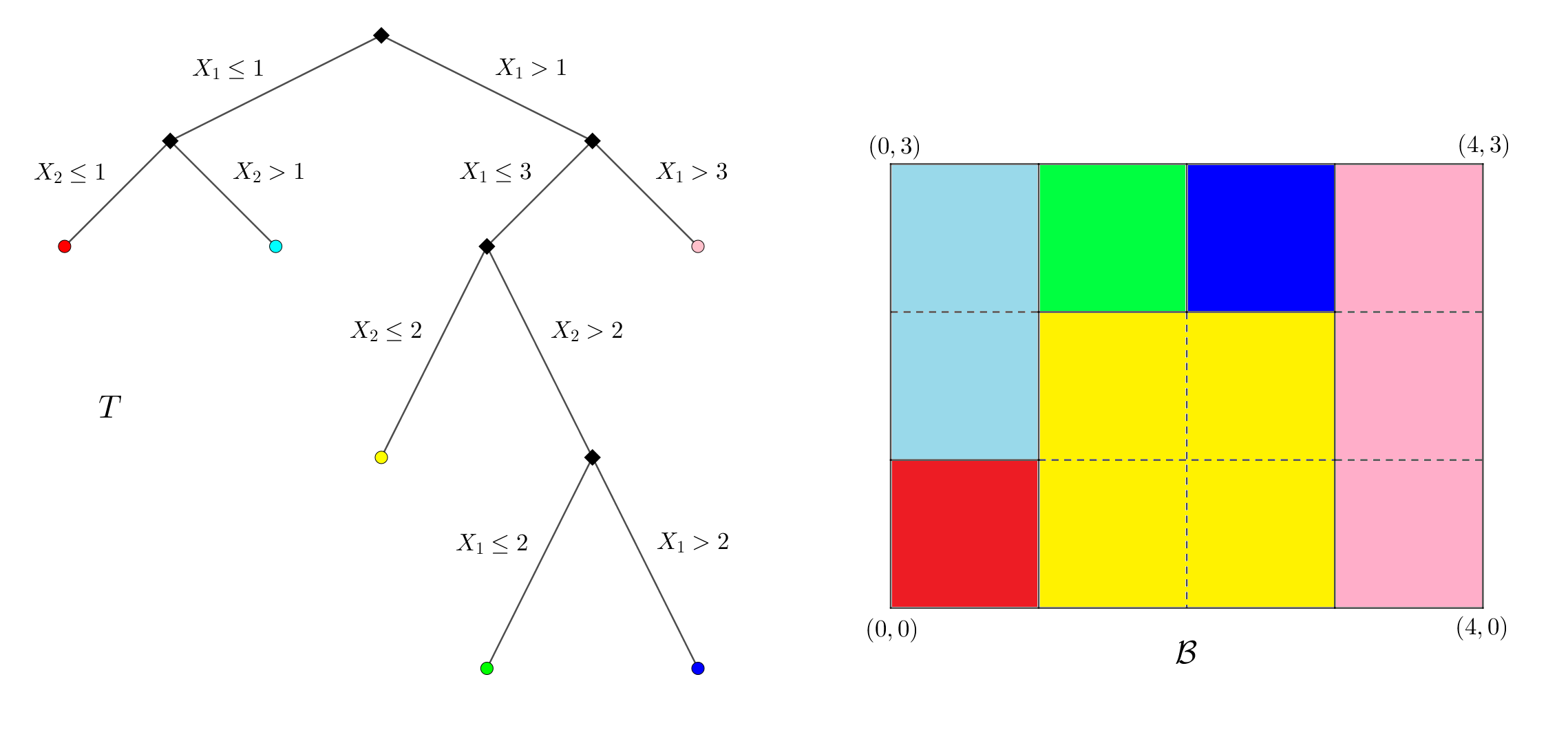
We now arrive at one of our main results which generalizes observations made after Example 3.1 by showing that, for a decision tree, marginal and TreeSHAP feature attributions are constant on each piece of the grid partition determined by the tree (see Figure 2). This fails for the conditional feature attributions as observed in Example 3.1.
Theorem 3.2.
With notation as in Sections 2.1, 2.4, let be a regression tree trained on data which implements a function . Consider the corresponding marginal
and TreeSHAP
games. Then for any linear game value and any , and are simple functions with respect to the grid partition away from the decision boundary1212 12 This is cut by all hyperplanes where splits on at some node. of whose -measure is zero due to (2.9). More precisely, away from the decision boundary:
- (1)
coincides with a linear combination of indicator functions with coefficients that are linear combination of elements of ;
- (2)
coincides with a linear combination of indicator functions with coefficients that are rational expressions of elements of where is the estimation based on data for the probability of ending up at the closed rectangular region :
(3.8)
A proof will be presented in Appendix D.1. The theorem also indicates that the feature attributions obtained from marginal and TreeSHAP games are very different functions. Indeed, for the former, one needs to compute/estimate probabilities , which in general cannot be recovered from the trained model since comes from a partition finer than what the tree determines. In contrast, is in terms of estimated probabilities . They become close to when the training set (assuming it is drawn i.i.d.) is large; see Lemma D.3. But even then, is different from since it can contain rational non-linear expressions of these probabilities.
3.3. Fewer features per tree: Implications to computing marginal values
In an ensemble of decision trees trained on features ,
only a portion of trees splits on a specific feature. By Lemma 2.1, that feature is a null player of the marginal game associated with any of the other trees.
Therefore, if one wants to quantify the contribution of as
via a linear game value such as Shapley or Banzhaf,
then only those decision trees which split on matter (due to the null-player property of ); and for those trees, one essentially deals with a game whose players are the features appearing in that tree (due to the carrier-dependence property of ).
To make this more precise, as in Section 2.4, write the trees in as
. Let denote the function computed by and
the one computed by ;
thus .
Denote the indices of features appearing in the decision tree , i.e. the features on which splits, by . Thus may be written as where is the projection operator.
Invoking Lemma 2.1, is a carrier for ; and for a game value of form (B.4) satisfying the carrier-dependence property:
| (3.9) |
The total number of summands in this double summation is no more than
However, applying directly to without utilizing the fact that not all features appear in all trees results in
which has summands. In the presence of a structural constraint which limits the number of distinct features per tree, can be much larger than the number of summands in (3.9).
Example 3.3.
Explainable Boosting Machines [52] are based on Generalized Additive Models plus Interactions [43]. In the boosting procedure, each tree is trained on one or two features. Hence the model computes a function of the form
where interaction terms are indexed by the subset of . With the knowledge of the constituent univariate and bivariate parts of the model, the marginal Shapley values can be computed easily:
This can be used to estimate the marginal Shapley values of an EBM model based on a background dataset.1313 13 The method predict_and_contrib returns the univariate and bivariate terms of an EBM model.
Remark 3.4.
Equation (3.9) remains valid for coalitional game values with the null-player and coalitional carrier-dependence properties, e.g. the Owen value which is known to be helpful in explaining ML models [48]. Nevertheless, for EBM models (discussed above), the marginal Owen values do not differ from Shapley since for a game with two players Shapley and Owen values always coincide. But for more complicated yet still constrained (in terms of number of features per tree) models like CatBoost (see below), partitioning features yields different marginal values (cf. Appendix F).
3.4. Marginal Shapley values for ensembles of oblivious trees
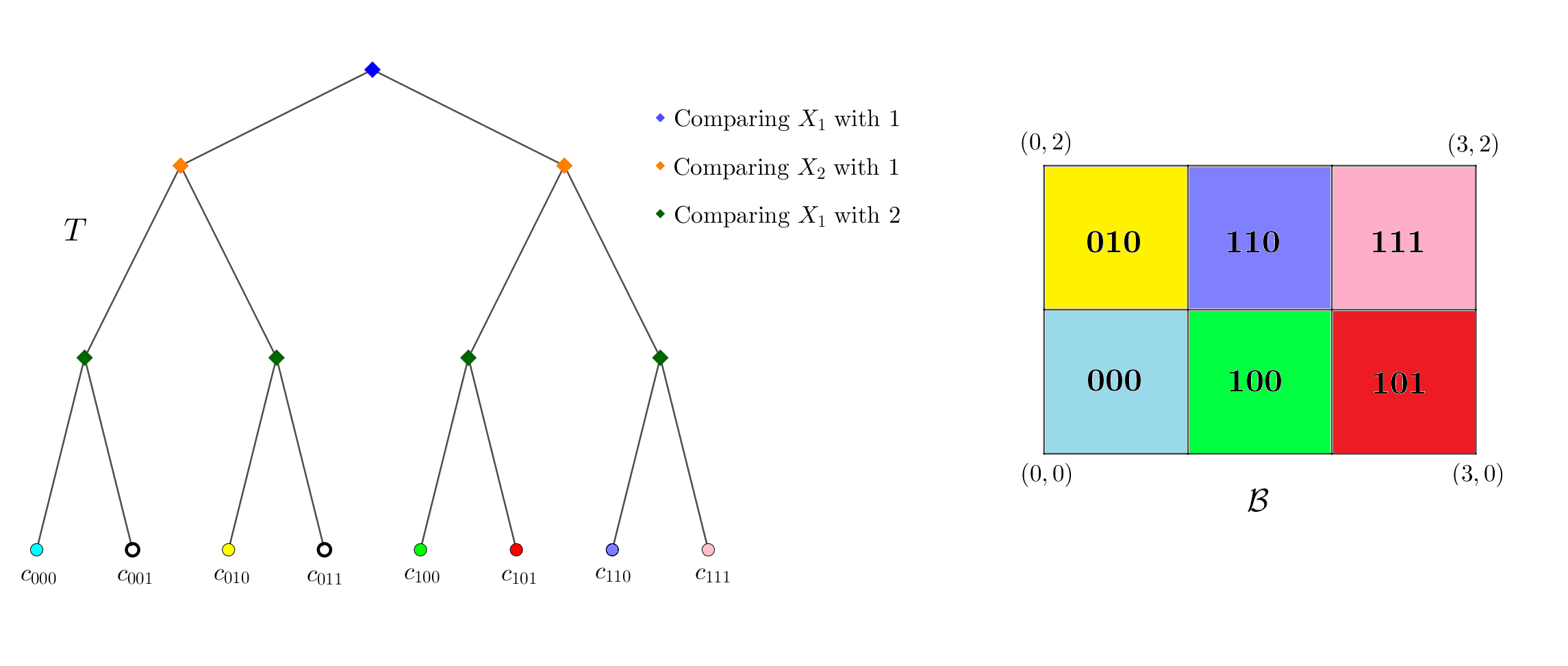
In previous sections, we observed that marginal feature attributions for a decision tree are piecewise constant functions, but with respect to the grid ; they do not necessarily remain constant on a region belonging to the original partition . The key observation of this section is that if is oblivious (cf. Definition 2.6), then . Invoking this and the symmetry of trees, we obtain a formula in terms of internal model parameters for marginal Shapley and Banzhaf values of ensembles of oblivious trees, e.g. CatBoost models. We first need some preliminary work before stating the theorem.
Definition-Notation 3.5.
Let be an oblivious decision tree of depth . Denote the distinct features appearing in from top to bottom by , say a subset of the ambient set of features . Starting from the root, suppose splits with respect to ( not necessarily distinct); and write the corresponding thresholds as —i.e. splits at all internal nodes of the level occur based on comparing with .
- •
We label each leaf with a binary code where, for the bit, amounts to while corresponds to . Any such code can also be thought of as a path from the root to a leaf.
- •
One has a partition of , indexed with elements of , where for any .
- •
When an oblivious tree splits on a feature more than once, some of the regions cut by the tree become vacuous; see Figure 3.1414 14 For instance, if splits on twice with thresholds and , then all regions with become vacuous (or of probability zero when because the event is of probability zero due to our assumption in (2.9).) A leaf is called realizable if the path to it from the root does not encounter conflicting thresholds for a feature. The corresponding set of realizable binary codes is denoted by . Regions encoded by elements of are vacuous (or of probability zero).
- •
We now define purely combinatorial functions parametrized by a partition of a segment of natural numbers. First, for binary codes , set
(3.10) Next, based on this, we define a function which takes in a binary code and a subset of as inputs:
(3.11)
Now consider where are the predictors and is a function implemented by an ensemble of oblivious decision trees. The notions discussed in Definition-Notation 3.5 can be considered for any arbitrary tree from the ensemble: We denote the depth by and the number of distinct features on which splits by . The leaves of are in a bijection with binary codes in ; the subset of realizable ones is denoted by . Moreover, the levels on which different features from appear determine a partition of size of which we denote by . The tree defines an inclusion
| (3.12) |
with the property that is the (enumerated from the root) distinct feature on which splits (i.e. in terms of the above notation). The corresponding element of captures all levels where splits with respect to . Moreover, belongs to the subset of trees splitting on a given feature if and only if is in the image of . Finally, for any leaf of encoded with , we denote the value at the leaf with , the corresponding rectangular region in with , and the probability of a data point ending up in that region with .
Theorem 3.6.
With the notation as above, for any and -almost every explicand , the marginal Shapley value of the regressor implemented by is given by
| (3.13) |
where is so that is satisfied. The terms inside the brackets in (3.13) are defined in terms of expressions1515 15 The quantity may be interpreted as an expectation: this is the expected leaf score taken over leaves that “partially” coincide with (in the sense of ) assuming that their scores are replaced with that of .
| (3.14) |
as
| (3.15) |
where , and the coefficients and are defined as
| (3.16) |
Via substituting (3.14) in (3.15), each of or can be obtained, through less than
| (3.17) |
multiplication operations, as a summation with no more than
| (3.18) |
summands, each of them a multiple of the product of two of parameters and which are associated with the leaves of . Thus formula (3.13) for computing has no more than
| (3.19) |
terms once expanded.
All these hold for the Banzhaf value too
after replacing coefficients
with
| (3.20) |
A proof can be found in Appendix D.2. The theorem can be formulated for game values introduced in Theorem 2.4 too, and also for coalitional game values such as the Owen value albeit it becomes tedious. So we skip it here and we refer the reader to Appendix F.
Remark 3.7.
Remark 3.8.
Notice the two speedups employed in the theorem. The summation in (3.13) only considers the trees relevant to the feature under consideration; and numbers , therein are described in summations (3.15) by focusing only on realizable binary codes which causes the number of summands to decrease when the tree has many repeated features.
Remark 3.9.
The complexity of computing marginal Shapley values for a symmetric tree via the previous theorem is sublinear in terms of the number of leaves once a restriction is posed on the number of distinct features on which the tree depends. This is because if as , then
Example 3.10.
The goal of this example is to verify Theorem 3.6 in the case of the symmetric tree of depth three illustrated in Figure 3. The features are supported in the rectangle which is partitioned into six subrectangles by the tree. Following Definition-Convention 3.5, we label the leaves of and their corresponding subrectangles with binary codes in . The set of realizable binary codes is of size six . The simple function computed by is
| (3.21) |
where
The feature appears on the first and third levels while appears only on the second level. This amounts to the partition
of which is indexed by . To obtain the set of realizable codes, all codes with the first bit and the third bit , i.e. codes and , should be excluded. Now suppose we want to compute the value that attains on one of the subrectangles, say on ; that is, . In (3.15), we are interested in pairs of elements of with
| (3.22) |
Since , we have and on the first line, and and on the second. As for the second bits, given that , they are determined based on if belongs to and or not. All possibilities for bits and are summarized in Table 3 along with the corresponding weights for these pairs as defined in (3.16). We now invoke Theorem 3.6 to compute where . In the first summation from (3.15), one should have , and the summation becomes
Notice that the three summands above correspond to the rows of Table 3. Next, in the summation from (3.15), to be subtracted from the former, one has and the summation becomes
Therefore, whenever . To verify this directly, notice that for the model (3.21) the first marginal Shapley value over is given by:
| (3.23) |
It is not hard to check that the above expression coincides with after simplification.
Example 3.11.
Let us apply Theorem 3.6 to an oblivious decision tree of depth which does not split on any feature on more than one level. With the notation as in Definition-convention 3.5, one has ; and the leaves, along with their values and their corresponding regions, can be encoded with elements of —all of them are realizable, i.e. coincides with . Enumerating the features appearing in the tree from the top as (all distinct), the resulting partition of coincides with the partition into singletons. It is easy to check that in this case has only one element, which, denoted by , is given by:
Now for any and , the followings holds for -a.e. point from the region :
Theorem 3.6 suggests a two-stage algorithm for approximating marginal Shapley values as the Shapley values of the empirical marginal game (2.2); this amounts to replacing the true probabilities associated with leaves with their estimations based on the training data:
| (3.26) |
Algorithm 3.12.
With the notation as in Theorem 3.6, suppose is a model computed by an ensemble of oblivious decision trees.
In the precomputation phase, for each leaf of each tree, the empirical marginal Shapley values
arising from that tree are computed for data points that end up at that leaf. These are recorded in look-up tables which are then used in the production phase to estimate the vector of marginal Shapley values for an input explicand.
First, should be parsed to obtain the following quantities used in the precomputation algorithm:
- •
functions enumerating features appearing in each tree;
- •
depths , distinct feature counts and partitions associated with the trees as well as leaf scores and estimated probabilities 1616 16 A code for “unpacking” a trained XGBoost, LightGBM or CatBoost model and retrieving quantities such as distinct features in each tree, depths, estimated leaf probabilities etc. is available on https://github.com/FilomKhash/Tree-based-paper.;
- •
combinatorial data .
-
Step 1 (precomputation).
-
Step 2 (computation). The outputs of the previous step are saved as look-up tables: one table for each tree whose rows are vectors of size . They then can be employed for explaining new data points on the fly as long as the model is in production.
In the implementation, the algorithm can be highly vectorized, and also parallelized across the trees in the ensemble (or even across the leaves of a single tree if necessary). Its complexity can be analyzed in light of inequality (3.19) for the number of terms in the formula for a marginal Shapley value of an oblivious tree. The aforementioned inequality yields the complexity
(in which the constant hidden in the notation is small).
But, for each tree, the precomputation algorithm goes through all leaves and all features on which the tree splits. This yields the total complexity
for precomputation and for storage of the look-up tables (again, with a small hidden constant).
To compare with path-dependent and interventional TreeSHAP algorithms (cf. Section 2.5) which do not conduct a precomputation, the complexity per leaf should be considered which is
.
All these facts are reflected in Table 1.
The complexity terms appearing therein for Algorithm 3.12 are elaborated on in Appendix D.2.
At the heart of the precomputation algorithm is the computation of a preimage
for each tree , where and
. The computational complexity, and that of its memory storage, is for each tree. These values are then used to compute the values
obtained in the first part of Step 1 of Algorithm 3.12, whose complexity is also for each tree, rather than
. The elements of are then used to compute the game value at every leaf and for every player; re-using the values multiple times is the main aspect of the precomputation algorithm, which helps to reduce overall complexity by sacrificing the memory storage.
Remark 3.13.
Suppose during the period that the ensemble is in production, the data distribution changes qualitatively. In such situations, assuming the same tree structures are kept, one can first update the leaf weights, and then redo the precomputation step of Algorithm 3.12 to update the look-up tables accordingly.
Remark 3.14.
By incorporating generalizations of Theorem 3.6 from Appendix F, Algorithm 3.12 can be modified to estimate those marginal feature attributions of CatBoost models that stem from a larger class of game values, or from coalitional game values such as the Owen value. The Owen values are indeed relevant since they can be used to recover the Shapley values of categorical features that were one-hot encoded before the training. We elaborate on this in Proposition B.13. This is one of the rare cases where Shapley values can be recovered after a non-linear transformation of features. It is infeasible to do something similar for the other highly complex built-in encodings of categorical features in the CatBoost library.
The last theorem of the section bounds the -error of the algorithm when it is applied to a dataset drawn i.i.d. from according to . In that setting, the estimated probabilities , now treated as random variables, converge to the true probabilities as (see Lemma D.3). Another quantity related to these probabilities that comes up in our error term is minus the Gini impurity; that is, the following quantity between zero and one associated with a tree:
| (3.27) |
In other words, is the sum of squares of probabilities that assigns to the regions cut by the decision tree .
Theorem 3.15.
Consider where are the predictors and the model is implemented via an ensemble of oblivious trees. Fix and denote the subset of trees that split on by . Suppose the dataset in Algorithm 3.12 is a random sample drawn i.i.d. from according to ; hence the (unbiased) estimator of the marginal Shapley value becomes a random variable. Then for -almost every one has
| (3.28) |
where, on the right-hand side, the second term is the maximum possible value for the -norm of the vector formed by the leaf scores1717 17 It is more precise to say “relevant” leaf scores because the leaves corresponding to degenerate regions are ignored. of a tree from which splits on ; and in the first term, we have the constant
| (3.29) |
which is no larger than with being the maximum possible number of leaves. In particular, for a fixed , in as the size of tends to infinity.
See Appendix D.2 for a proof.
Remark 3.16.
Recall that the estimations of Shapley values generated by the algorithm above coincide with the Shapley values of the empirical marginal game defined based on the training set, i.e. in the above setting. Thus, due to (2.2), the estimator is an average of i.i.d. random variables, making Theorem 3.15 essentially a consequence of the Strong Law of Large Numbers [40].
Remark 3.17.
Theorem 3.15 establishes strong convergence of the estimator, which implies convergence in probability [40]. In particular, (3.28) and the Chebyshev inequality [40] imply for any threshold that
| (3.30) |
where is the multiplier of on the right-hand side of (3.28). Thus, given any , one can always pick the number using the bound (3.30) such that the estimator based on falls in the interval with probability at least whenever .
Remark 3.18.
To get from the Lipschitz constant (3.29) to the cruder one , the term was replaced with . But the reader should keep in mind that, in principle, can be as small as .
Remark 3.19.
The inequality (3.28) holds for -a.e. . It thus yields an upper bound for the mean integrated squared error (MISE) of the estimator as well.
4. Numerical experiments
This last part is devoted to our experiments with data. The claimed complexity of the algorithm (see Table 1) is verified in Section 4.1 through working with a synthetic dataset; and its performance is moreover benchmarked with TreeSHAP (cf. Figure 4 and Figure 5). Next, in Section 4.2, we train CatBoost, XGBoost and LightGBM models on four public datasets. We compute and compare various quantities pertinent to the structure of trees (cf. Table 6) to showcase some of the points previously made. Next, in Section 4.3, we apply Algorithm 3.12 to the four CatBoost models trained in the preceding section to compute their marginal Shapley values, and we record the time (cf. Table 7).
We refer the reader to Appendix A for more on the data and codes used for this section.
4.1. Complexity of Algorithm 3.12
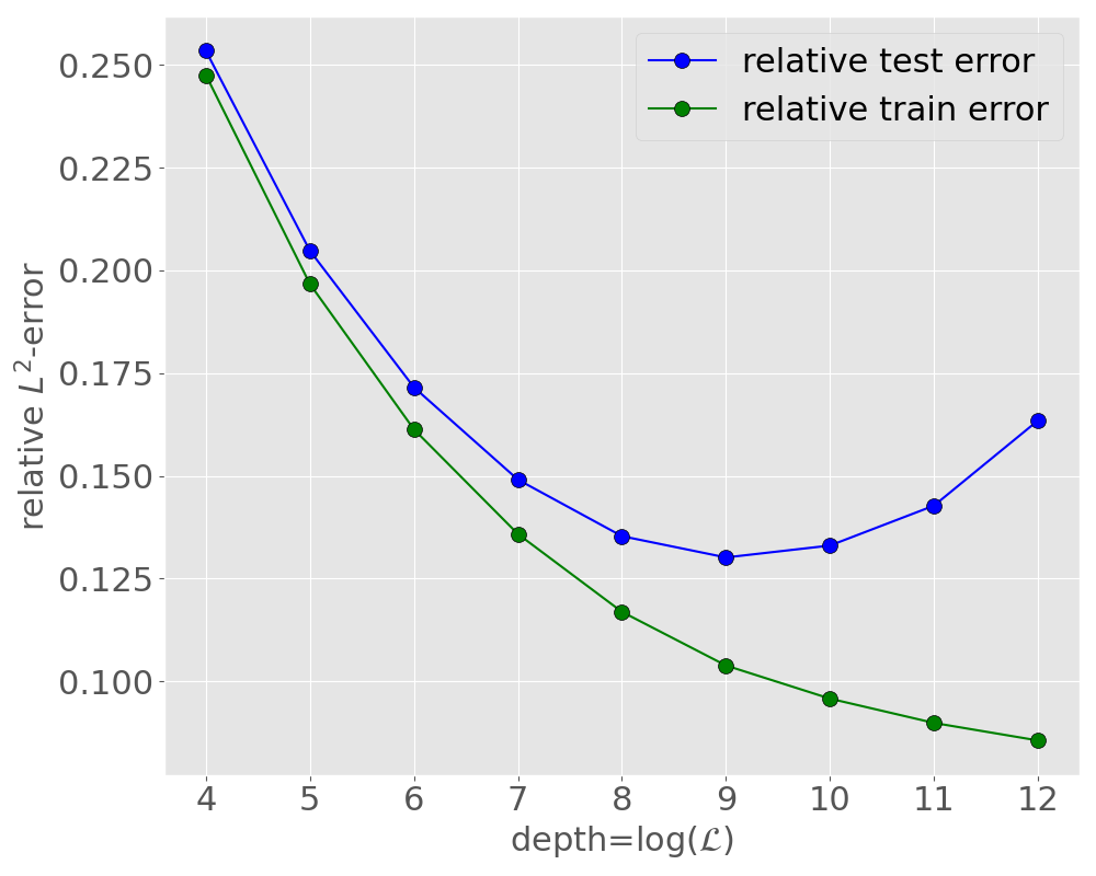


In this section, we use a synthetic dataset to investigate the complexity of Algorithm 3.12, both precomputation and computation steps, in terms of the maximum number of leaves in a CatBoost ensemble.
Suppose the predictors obey the normal distribution
where is the identity matrix. The model for the response variable is assumed to be:
| (4.1) |
where and are coefficients in intervals and chosen randomly (once); and , with , is a noise term.
For our numerical experiment, we generated samples drawn from the data generating model (4.1) with . We then trained a collection of CatBoost regressors where the max_depth parameter is set to be respectively (which in turn yields ensembles with the maximum number of leaves, , being respectively). Other tuned training hyperparameters are: n_estimators, subsample, learning_rate. A subset of samples drawn from (4.1) was used as the test set.
The relative -errors for training and test sets are depicted on Figure 4(a).
We then carried out Step 1 of Algorithm 3.12 on an AWS machine with 32 cores and 256GB of memory. This step precomputes marginal Shapley values at every realizable leaf of each tree, relying only on the internal parameters of trained models, and without taking in any background dataset. For these nine models, the average precomputation time, per tree in the ensemble, is plotted in Figure 4(b) in the logarithmic scale. Recall from Section 3.4 that the theoretical complexity of the precomputation algorithm should be ; compare with Table 1. The true complexity observed on Figure 6, however, can be expressed in the form where depends on the depth of the tree and varies from for small depths to for depth equal to . As the depth increases, we expect that the complexity curve would tend to a straight line with the slope .
We remind the reader that the precomputation occurs only once. Its results, the (local) game values associated with every realizable leaf of each tree in the ensemble, are saved in look-up tables.
These are then used in Step 2 (on-the-fly computation step) of Algorithm 3.12 to output the vector of Shapley values for any input data point.
We performed this step for randomly picked samples of the training set for each of the models. The average computation time per observation for these nine models is depicted on Figure 4(c). As expected from Table 1, the complexity is linear in terms of .
We next compare Algorithm 3.12 with the interventional TreeSHAP algorithm which requires a background dataset as an input. Background datasets of sizes , , , and were used for this part. Unlike [44], we avoid using small background datasets with a few hundred samples since, for them, the relative statistical error can be quite high (for details, see [41]).
To estimate marginal (interventional) Shapley values for them, the get_feature_importance method of CatBoost, with the default setting shap_calc_type="Regular", was used.
According to the documentation, this implements the interventional TreeSHAP algorithm [44].1818
18
Check https://catboost.ai/en/docs/concepts/python-reference_catboost_get_feature_importance.
Figure 5(a) illustrates the average computation time of our inherently interpretable algorithm (Step 2 of Algorithm 3.12) compared to the interventional TreeSHAP with the aforementioned background datasets.
As expected from Table 1, the latter are exponential in terms of whereas the former is linear, and thus much faster.
As for the precomputation time of our algorithm (Step 1 of Algorithm 3.12), comparison with the execution times of interventional TreeSHAP is, in general, difficult. However, renormalizing the precomputation time on the average number of leaves of trees in the ensemble is, in principle, comparable to the computation times per observation of the on-the-fly algorithms.
For ensembles , Figure 5(b) compares the precomputation times per leaf (that is, the precomputation time divided by the average number of leaves in any given tree) with the computation times of algorithms that require background datasets. We note that the accuracy of Algorithm 3.12 corresponds to the empirical marginal Shapley value based on the training set which has samples, much larger than the background datasets. Meanwhile, our precomputation per leaf is only a few times slower than the on-the-fly computation by the interventional TreeSHAP.
Finally, after the first draft of this paper appeared on arXiv, we discovered that the CatBoost method get_feature_importance allows for the argument shap_calc_type to be set to "Exact" and shap_mode to be set to "UsePreCalc". It appears that
these options allow for the precomputation at every leaf of each tree, and subsequently allow for the evaluation of explanations at every given observation based on the precomputed information.
No detailed documentation on what these options are, or error analysis (such as Theorem 3.15) is available at the time of writing. Furthermore, the two steps cannot be run independently, which unfortunately limits the use of the "UsePreCalc" option.
Nevertheless, to make our treatment comprehensive, we compared the precomputation time of our algorithm with the native CatBoost one (where we simply provided a single explicand).
Figure 6 illustrates the time comparison in terms of the number of leaves, both with and without the logarithmic scale. Notice that ours (Step 1 of Algorithm 3.12) is faster; and its complexity is linear in the logarithmic scale in accord with our theoretical analysis (cf. Table 1).
The plot hence shows that the two methods are different.
At last, it must be mentioned that our proposed algorithm can be generalized to any other game value characterized by Theorem 2.4, or even to certain coalitional game values such as the Owen value; see the results of Appendix F.
To the best of our knowledge, no competitor algorithm presents a similar option.
Indeed, we repeated our experiments for generating the marginal Shapley values for CatBoost models trained on synthetic data (4.1), this time for the marginal Owen values, based on a proprietary code that computes these values in a two-stage procedure similar to Algorithm (3.12). Figure 7 illustrates computation and precomputation times.


4.2. Experiments with public datasets
For this section, we trained models on public datasets through libraries that construct trees very differently.
The datasets used are the Superconductivity dataset [28],
the Ailerons dataset [70], the Online News Popularity dataset [23],
and the Higgs dataset [73]. Table 4 outlines the task, the number of variables and the sizes for training, validation and test sets for each of them. The features are non-categorical in all cases. See Appendix A for descriptions of these datasets.
For each dataset, we trained a CatBoost, a LightGBM and an XGBoost model with the libraries’ default growth policies.
Their performances over the test set, recorded in Table 5, indicate that
each model enjoys a reasonable predictive power;
and their outputs are much closer to each other than to the ground truth.
But the models’ internal structures differ considerably in the sense that their constituent trees are topologically very different. This is observed in Table 6 where we disentangle each ensemble to obtain quantities such as the average number of leaves, the average number of distinct features per tree etc.
Based on the table, and following the same notation, we observe that:
- (1)
Comparing the number of leaves with its maximum possible value indicates that, overall, the trees in LightGBM ensembles are sparse while those in CatBoost ensembles are prefect binary (as expected); XGBoost ensembles lie some place in between.
- (2)
On average, the number of distinct features is smaller than the maximum possible number of features appearing in the tree , i.e. the depth in the case of CatBoost models and the number of internal nodes for trees from XGBoost and LightGBM ensembles.1919 19 In training, the number of features used for constructing a tree was not limited by any hyperparameter (i.e. a hyperparameter such as colsample_bytree in XGBoost and LightGBM was not used). This indicates that trees occasionally split more than once with respect to some feature (or some feature appears on more than one level in the case of CatBoost).
- (3)
Following the discussion in Section 3.3, for game values with null-player and carrier-dependence properties such as Shapley and Banzhaf, only the trees that split on a given feature matter for computing its marginal attribution. Furthermore, the contribution of each of those trees to the feature attribution under consideration depends only on the distinct features appearing in that tree. Now, revisiting Table 6, we first observe that is often much smaller than ; namely a feature appears only in a portion of trees from the ensemble. Secondly, the total number of variables, , is much larger than the average number of distinct features per tree . All in all, we observe that , where is the complexity of naively computing a game value such as Shapley for players. This reinforces one of this paper’s key points: For tree ensembles, the complexity of computing marginal feature attributions such as Shapley, Banzhaf or Owen can be lowered through taking individual trees and their structures into account; see (3.9).
- (4)
Recall that Theorem 3.2 puts forward a method for estimating the vector of marginal Shapley values of a CatBoost model at an explicand. These are generated based on the whole training set and with complexity where is the maximum possible number of leaves (compare with Table 1). To get estimations with a comparable accuracy from the interventional TreeSHAP, take the training set as the background dataset. According to (2.13), the complexity would then become . This is a much higher complexity: Table 6 indicates that, for CatBoost models we trained on datasets from Table 4, the ratio is always larger than .
| Dataset | Task | Features | Train | Validation | Test |
| Superconductivity [28] | Regression | 81 | 12,757 | 4,253 | 4,253 |
| Ailerons [70] | Regression | 40 | 5,723 | 1,431 | 6,596 |
| Online News [23] | Classification | 58 | 23,786 | 7,929 | 7,929 |
| Higgs [73] | Classification | 28 | 10,000,000 | 500,000 | 500,000 |
| Superconductivity | Ailerons | |||||||
| 1 | 0.9905 | 0.9788 | 0.9206 | 1 | 0.9678 | 0.9347 | 0.8297 | |
| 0.9904 | 1 | 0.9814 | 0.9212 | 0.9694 | 1 | 0.9499 | 0.8336 | |
| 0.9780 | 0.9809 | 1 | 0.9166 | 0.9409 | 0.9524 | 1 | 0.8003 | |
| Online News | Higgs | |||||||
| 1 | 0.8695 | 0.8324 | 0.7324 | 1 | 0.9420 | 0.9460 | 0.8465 | |
| 0.8786 | 1 | 0.8668 | 0.7328 | 0.9461 | 1 | 0.9533 | 0.8402 | |
| 0.8259 | 0.8512 | 1 | 0.7238 | 0.9473 | 0.9511 | 1 | 0.8409 | |
| Dataset | model type | ||||||
| Superconductivity | CatBoost | 300 | 27.70 | 256∗ | 8∗ | 7.48 | 81 |
| LightGBM | 300 | 85.48 | 31∗ | 11.48 | 23.08 | ||
| XGBoost | 300 | 92.69 | 42.21 | 6∗ | 25.03 | ||
| Ailerons | CatBoost | 50 | 7.50 | 126.72 | 6.98 | 6.00 | 40 |
| LightGBM | 50 | 14.00 | 25∗ | 8.42 | 11.20 | ||
| XGBoost | 40 | 1.98 | 3.78 | 1.85 | 1.98 | ||
| Online News | CatBoost | 167 | 19.86 | 128∗ | 7∗ | 6.90 | 58 |
| LightGBM | 88 | 32.78 | 31∗ | 10.41 | 21.60 | ||
| XGBoost | 88 | 26.98 | 27.09 | 5∗ | 17.78 | ||
| Higgs | CatBoost | 1000 | 251.32 | 256∗ | 8∗ | 7.04 | 28 |
| LightGBM | 1000 | 636.68 | 60∗ | 13.18 | 17.83 | ||
| XGBoost | 1000 | 524.93 | 31.89 | 5∗ | 14.70 |
4.3. Applying Algorithm 3.12 to models from Section 4.2
For this section, an implementation of Algorithm 3.12 was applied to the four CatBoost models from Section 4.2.
To this end, a proprietary, internal library based on Algorithm 3.12 (and its generalizations; cf. Appendix F) was used.
This library generates accurate estimations of marginal Shapley (as well as Banzhaf, Owen etc.)
feature attributions for ensembles of oblivious trees without reliance on any background dataset.
The execution time for the precomputation step, as well as the time required for generating Shapley values for 100 random test samples,
are recorded in Table 7. Observe that the algorithm is very fast.
Similar execution times for the Owen value are available from Table 8.
The look-up tables constructed for these CatBoost models are available on https://github.com/FilomKhash/Tree-based-paper
along with a code which provides a sanity check via verifying the efficiency property of Shapley
and Owen values. We refer the reader to Appendix A for more on our experiments and the relevant material.
| Dataset | Features | Trees | Precomputation (no multithreading) | Precomputation (with multithreading) | Total Size | Computation (100 samples) |
| Superconductivity | 81 | 300 | 20.118s | 6.197s | 10.6MB | 0.030s |
| Ailerons | 40 | 50 | 0.600s | 0.367s | 808KB | 0.005s |
| Online News | 58 | 167 | 3.518s | 1.888s | 3.19MB | 0.017s |
| Higgs | 28 | 1000 | 51.140s | 19.152s | 32.3MB | 0.068s |
| Dataset | Features | Trees | Partition Size | Precomputation (no multithreading) | Precomputation (with multithreading) | Total Size | Computation (100 samples) |
| Superconductivity | 81 | 300 | 11 | 32.022s | 10.138s | 10.6MB | 0.034s |
| Ailerons | 40 | 50 | 24 | 2.059s | 1.025s | 808KB | 0.006s |
| Online News | 58 | 167 | 37 | 12.827s | 3.715s | 3.19MB | 0.015s |
| Higgs | 28 | 1000 | 27 | 252.005s | 61.908s | 32.2MB | 0.068s |
Appendix A Availability of data and code
Here, we elaborate on the experiments that we carried out for this paper, and on the supplementary material which is available from https://github.com/FilomKhash/Tree-based-paper.
The computations in Example 3.1 concerning path-dependent and interventional TreeSHAP for decision trees from Figure 1 are confirmed in the notebook TreeSHAP_Sanity_Check.ipynb.
In Sections 4.2,4.3, we deal with models trained on the following public datasets; also see Table 4.
- (1)
The Superconductivity dataset [28]: a regression dataset where the superconductivity critical temperature should be predicted based on 81 features extracted from the superconductor’s chemical formula. The original dataset has 21,263 instances. We randomly split it into training, validation and test sets in 60:20:20 proportions.
- (2)
The Ailerons dataset [70]: a regression dataset originating from a control problem for an F-16 aircraft where the control action on the ailerons of the aircraft should be predicted based on 40 features describing the status of the airplane. The original data comes in a test set with 6,596 instances and a training set with 7,154 instances. The latter was split into a smaller training set and a validation set in 80:20 proportions.
- (3)
The Online News Popularity dataset [23]: a dataset with features about articles published in a period of two years on the news website Mashable. We used it for a binary classification task where one should predict if an article has been shared at least 1,400 times in social networks or not. The prediction should be done based on 58 features (two of the features from the original dataset are non-predictive). The data we obtained from the data source had 39,644 instances. We randomly split it into training, validation and test sets in 60:20:20 proportions.
- (4)
The Higgs dataset [73]: a binary classification dataset where, based on 28 features that are functions of the kinematic properties, one should distinguish between a signal process which produces Higgs bosons and a background process which does not. The original dataset has 11,000,000 instances; and the data source states that the last 500,000 instances should be used as the test set. We randomly picked 500,000 instances from the rest as the validation set.
As mentioned in Section 4.2, for each of the datasets above, we trained a CatBoost, a LightGBM and an XGBoost model. These models are available on the GitHub repository along with the notebook r2_score.ipynb which replicates the metrics for them as outlined in Table 5. Moreover, the quantities in Table 6, which are related to the structure of trees in these models, were generated with the code in Retrieve_splits.ipynb. The notebook contains three functions retrieve_catboost, retrieve_lgbm and retrieve_xgb which respectively parse a trained CatBoost, LightGBM or XGBoost decision tree to extract information such as depth, number of leaves, distinct features on which the tree splits, thresholds for splits, and the rectangular regions corresponding to leaves along with their associated probabilities and values. Notice that such information is a prerequisite for applying Algorithm 3.12 to CatBoost models. We have furthermore included a script EnsembleParser.py on the GitHub repository which can be used to obtain such statistics for an arbitrary trained CatBoost, LightGBM or XGBoost model.
For Section 4.3, a proprietary, optimized implementation of Algorithm 3.12 was applied to the four CatBoost models from Section 4.2 (trained on public datasets) on an AWS machine with 16 cores and 128GB of memory. The code for the precomputation step uses the package Numba for just-in-time (JIT) compilation, and can also leverage multithreading. The execution times for the precomputation step of Algorithm 3.12 are recorded in Table 7, both with and without multithreading (the JIT compilation time, which was less than seven seconds, is not included). The table also includes the time it took to compute Shapley values for a random subsample of size 100 in the second step of the algorithm via utilizing the look-up tables generated in the first step. The total size of these tables on disk can also be found there. Since our internal library is not available on GitHub, we provide a sanity check to confirm that the look-up tables indeed contain Shapley values. This is done through verifying the efficiency property of Shapley values of a machine learning model (see Example B.6) in explanations.ipynb. The code in this notebook randomly picks a tree from the CatBoost ensemble and a leaf of that tree, and then verifies that, at that leaf, the sum of Shapley values of features appearing in the tree agrees with the leaf’s output minus the average of all leaf values (i.e. the average of raw predictions of that decision tree over the training set). For the same four CatBoost models, we also present execution times for computing the Owen values in Table 8 of Section 4.3. For each of the four public datasets, the partition of variables which underlies the Owen value generation was obtained through hierarchical clustering of variables based on maximal information coefficient [55]. The notebook grouping.ipynb details this process. This is also available on our GitHub repository along with the partitions used for Table 8 as json files. The look-up tables constructed for Owen values are available as well, and again the efficiency property may be verified for them as a sanity check.2020 20 The second part of Proposition E.2 along with the efficiency property of the Shapley value immediately imply that the identity appearing in Example B.6 carries over to the marginal or conditional Owen values of a model.
The experiments in Section 4.1 were designed to benchmark the complexity of our internal explanation library with other explanation methods. The comparison was done for CatBoost models of varying depths trained on a synthetic dataset generated by (4.1). The code was run on an AWS machine with 32 cores and 256GB of memory. The reader can find the execution times of our proprietary code on the GitHub repository along with scripts plotter.py and plotter_owen.py for recreating figures of Section 4.1.
Appendix B Background from game theory
B.1. Properties of game values
The goal of the current section is to briefly review basic concepts from cooperative game theory and various properties of game values.
Let be a finite non-empty subset of and denote its cardinality by .
An -person game with as its set of players is a set function ;
is called a cooperative game if . A game value is a function that to any cooperative game assigns a vector .
We first review some important properties of game values.
Definition B.1.
Let be a game value; that is, an assignment where varies among cooperative games.
- •
The game value is linear if for any scalar and any two cooperative games and with the same set of players .
- •
An element is called a null (dummy) player for if for any . We say satisfies the null-player property if whenever is a null player.
- •
A carrier for a game is a subset with the property that for any ; namely, a subset whose complement consists of null players. The game value satisfies the carrier-dependence property if for any carrier of a game one has for all . (On the right-hand side, is applied to the restrictions of the original game to .)
- •
The game value satisfies the efficiency property if
(B.1) for any cooperative game .
- •
The game value satisfies the symmetry property if for any game and any permutation of one has for all where is defined as . Equivalently, is symmetric if and only if for any game and any :
(B.2) - •
The game value satisfies the strong monotonicity property if for any two games and any :
(B.3)
As mentioned before, this article mostly deals with games where and with game values defined explicitly by a formula of the form (1.3) (where was replaced with to simplify the notation). The next lemma justifies our convention (also see Remark B.4).
Lemma B.2.
Linear game values with the null-player property are precisely those that can be written as
| (B.4) |
where is a cooperative game and is a real-valued function defined on the set of subsets of . Furthermore, for a game value of this form, properties from Definition B.1 can be rephrased as:
- (1)
carrier dependence for all and ;
- (2)
efficiency & ;
- (3)
symmetry there exists a function with for all and ;
- (4)
strong monotonicity .
Proof.
If is linear, then, given any finite subset , there exist constants in terms of which the outputs of for any cooperative game may be written as
The equation above may be rewritten as
| (B.5) |
(Keep in mind that .) If is a null player for , then the first summation vanishes. Hence satisfies the null-player property if and only if for any cooperative game for which is a null player. But this happens exactly when all coefficients are zero since, in the former sum, each term can be any arbitrary real number. Substituting in (B.5) and setting , we arrive at the formula
for linear game values that satisfy the null-player property. Conversely, any game value of the form above clearly has the null-player property. This establishes the first claim. So we assume that is of the form above for the rest of the proof. Now let be a carrier for and . In the formula above, and can be replaced with and respectively. Thus
For to satisfy the carrier dependence, the above expression must always coincide with
thus the equality of corresponding coefficients:
(which always holds when ).
Next, we turn into part (2). For a game value of the form (B.4),
the efficiency property (B.1) turns into
where is a cooperative game, i.e. . The left-hand side may be rewritten as
This must agree with for any cooperative game . But, as varies among cooperative games , can be any element of . Therefore, the efficiency holds precisely when in the last expression the coefficient of is and the rest of the coefficients are :
As for the symmetry property, for any permutation of the set of players , one has
Comparing with the formula (B.4) for , the symmetry is equivalent to the equality of corresponding coefficients, i.e. for any permutation . This happens exactly when depends only on the cardinality of the proper subset of because for any two pairs
with ,
there exists a permutation of with and .
At last, we characterize the strong monotonicity property for game values of form (B.4).
Due to linearity, (B.3) amounts to
whenever all differences are non-negative. This amounts to for any since any such vector can be realized as for a suitable cooperative game . Clearly, the former inequality holds for all vectors with non-negative entries if and only if all the coefficients are non-negative. ∎
Remark B.3.
There is a systematic way of extending linear game values so that they can be applied to non-cooperative games as well [48, Section 3.5]. Indeed, conditional and marginal games associated with as in (1.1) are not cooperative since they assign to . But, a benefit of working with a formula such as (B.4) is that it remains unchanged after replacing a game with the cooperative one . In other words, (B.4) automatically extends2121 21 Extensions of the form to non-cooperative games are called centered. to non-cooperative games; and we shall freely apply such game values to marginal and conditional games. All properties appeared in Definition B.2 generalize to the case of non-cooperative games in an obvious way except the efficiency property which should be replaced with
| (B.6) |
Remark B.4.
The carrier-dependence property from Definition B.2 naturally brings up games whose sets of players are not necessarily segments of . On the other hand, it is tempting to define game values only for games with as in (1.3) rather than working with the more precise form (B.4). To alleviate this problem, notice that if a game value of form (1.3)—which is defined only in the case of —is symmetric, then by Lemma B.2 its weights depend only on the cardinality of . It can thus be unambiguously applied to any game by setting where is an arbitrary bijection.2222 22 This extension to games with arbitrary is unique if one imposes an isomorphism invariance axiom which is stronger than the symmetry axiom and requires for any game and any bijection .
Remark B.5.
The famous characterization of the Shapley value in [62] as the unique linear game value satisfying null-player, symmetry and efficiency properties can also be recovered from Lemma B.2: substituting from part (3) in the equations from part (2) implies that
From these, one can inductively show that is equal to ; consequently, coincides with the right-hand side of (2.3).
B.2. Marginal and conditional games
The marginal and conditional games associated with predictors and a Borel-measurable are defined as pointwise games in (1.1). Of course, they (along with feature attributions arising from them) can also be treated as random variables which, by abuse of notation, we denote as
| (B.7) |
where belongs to the sample space .2323 23 Any slice of a Borel-measurable function is Borel measurable too. Thus, fixing , is a random variable on and it thus makes sense to speak of its expectation in (B.7). In order for the expectations in (B.7) (conditional or unconditional) to exist, we always assume that the predictors belong to and is uniformly bounded on .2424 24 Lipschitz-continuous functions work too although is not continuous in our context.
Example B.6.
For these games, the efficiency property (B.6) turns into
| (B.8) |
for the marginal and conditional Shapley values.
Example B.7.
For a linear model , marginal and conditional Shapley values (treated as random variables here) are given by
and
Notice that the latter contains conditional expectation terms while the former is purely in terms of coefficients of the model . Moreover, if the predictors are independent, the two kinds of explanations coincide since all terms , and become or . Finally, the identities above showcase why in Lemma 2.1 certain assumptions on predictors are required in the case of the conditional game. When , the variable is absent from , and we see that the marginal Shapley value vanishes. This does not hold for its conditional counterpart unless is independent of the rest of variables. On the other extreme, when is the only non-zero coefficient, does not become a carrier for , i.e. in general. This is because the conditional expectations are not necessarily the same as unless a further assumption, e.g. the independence of from , is imposed.
Proof of Lemma 2.1.
If is independent of variables indexed by elements outside of , then
which implies that is a carrier. In particular, elements of are null players. As for the other claim of part (1), notice that the term above may be written as
For the second part, we shall need the following fact: Given random vectors and , one has provided that is independent from . Writing as again, if is independent of , then one has
The remaining claim follows immediately by setting : If does not depend on and is independent of , then is a carrier for the conditional game, and hence should be a null player. ∎
Remark B.8.
The marginal framework for feature attribution is sometimes called interventional because it can be thought of as enforcing independence between two complementary subsets of features and through causal intervention [33]. This amounts to a flat causal graph, not a general DAG (Directed Acyclic Graph), so the name can be misleading [10, p. 7].
B.3. Coalitional game values
A coalitional game value takes a cooperative game along with a partition of as inputs and returns a vector . Just like (B.4), it is convenient to assume that is in the form
| (B.9) |
which is linear and satisfies the null-player property in a clear sense.
The most important example for us is the Owen value (2.8) which is of this form.
The efficiency property from Definition B.2 immediately generalizes to coalitional game values, and it is not hard to see that it holds for the Owen value.
On the other hand, formulating symmetry or carrier-dependence properties for coalitional game values is slightly more subtle.
Definition B.9.
Let be a coalitional game value.
- •
We say that has the coalitional symmetry property if given a game and a partition of one has the followings:2525 25 These properties also come up in a characterization of the Owen value in [53].
- (1)
for any permutation of (i.e. the order of members of does not matter);
- (2)
for any permutation of .
- (1)
- •
We say that has the coalitional carrier-dependence property if given a game , a carrier , and a partition of , one has for all where is a partition of .
Lemma B.10.
The Shapley value and the Banzhaf value satisfy the carrier dependence property; and the Owen value satisfies the coalitional carrier dependence property.
Proof.
According to part (1) of Lemma B.2, to establish the carrier dependence for the Shapley value (2.3), it suffices to show that
for any finite subset of containing and any .
The left-hand side may be rewritten as
;
the result now follows from Lemma D.1.
Similarly, for the Banzhaf value, the identity from part (1) of Lemma B.2 holds:
For the carrier-dependence property, we refer the reader to Proposition E.2 where the coalitional carrier-dependence is established for a family of coalitional values generalizing the Owen value. ∎
We finish this section by discussing the quotient game and the quotient game property. In the context of Explainable AI, these game-theoretic concepts are used in [48] to unify marginal and conditional feature attributions of a model through appropriate groupings of predictors, and also to address the instability of the former type of attributions. For a game and a partition of its set of players , the quotient game has as its set of players and is defined as
| (B.10) |
A coalitional game value is said to admit the quotient game property if one has
| (B.11) |
for all and .
Example B.11.
The two-step Shapley value defined in [37]
| (B.12) |
has the coalitional symmetry and quotient game properties, but it does not satisfy the coalitional carrier-dependence or the null-player properties.
B.4. An application to categorical variables
In this short section, we argue that concepts such as a coalitional game value or quotient game
naturally emerge in the context of machine learning explanations when
it comes to one-hot encoding.
Let us first formalize the setting. Write the predictors as
| (B.13) |
where , a subset of size , captures the indices of categorical feature. Denote the range of the categorical feature , , by the finite set which can be indexed by . The one-hot encoding of yields a vector of random variables taking values in :
| (B.14) |
Therefore, the set of predictors after the encoding is
| (B.15) |
These are defined on the same probability space , and can be indexed with the elements of the disjoint union
| (B.16) |
Given a model , its transformed version takes points as inputs where and . It should yield the same output as the original model :
| (B.17) |
where each is the standard basis vector whose only non-zero entry is , located at the dimension . Notice that, above, the one-hot encoding was done as
| (B.18) |
We next relate the marginal game defined based on the original predictors and model to the marginal game associated with the encoded predictors and the transformed model. The set of players for the former is while the set of players for the latter is the set from (B.16). This set admits a natural partition . Its elements are in a one-to-one correspondence with elements of . Consequently, the set of players for both and the quotient game can be identified with .
Lemma B.12.
With the notation and convention as above, for any we have almost surely.
Proof.
Let us treat and as random variables on as in (B.7). Thus for any one has , and
| (B.19) |
where the definition of the quotient game, (B.10), was invoked. Due to the fact that each is obtained from one-hot encoding of the categorical feature as in (B.14), , with probability , is equal to a standard basis vector in . Equation (B.17) now implies that the right-hand side of (B.19) is the same as with probability . ∎
We are finally in a position to present an application to feature attributions in machine learning. Suppose a model is trained using the encoded features , but we want to recover the marginal Shapley values of the original categorical features . A common misconception is that, to this end, the Shapley values of the encoded features should be added up. The correct answer is to “enrich” the Shapley value to its coalitional counterpart, the Owen value. This can be generalized to the game values from (2.7) which mimic the Shapley value: To obtain marginal attributions based on for a categorical feature from the attributions of its encodings, one should employ coalitional analogs of —see Appendix E.2—that imitate the definition of the Owen value.
Proposition B.13.
With the notation and convention as above, we have
where is obtained from after the one-hot encoding, as in (B.18).
More generally, consider a game value ,
defined as in Theorem 2.4 based on a collection
of numbers satisfying (2.6). One then has
where is the coalitional game value defined as in (E.6) with and .
Appendix C Computations related to TreeSHAP
C.1. Computations for Example 3.1
Let us elaborate by first discussing the case of conditional and marginal games which are defined as in (1.1). It is convenient to write the function implemented by and as
| (C.1) |
One then has
| (C.2) |
Conditioning on which of , , or the point belongs to, the difference of expressions above can be written in terms of and functions from (3.2), hence the first row Table 2. As for the marginal game, plugging (C.1) in the definition yields
| (C.3) |
Probabilities appearing above can be written in terms of probabilities (3.3) assigned to subrectangles visible in Figure 1.
Simplifying the difference of expressions from (C.3) then yields the second row of
Table 2.
Based on Definition 2.8, the TreeSHAP games associated with and are given by
| (C.4) |
Their differences are recorded in the last two rows of Table 2. In particular, over , where and , the differences become
and
For the parameters in (3.5), the former is negative while the latter becomes positive. At the same time, the impurity measures are very close for the two trees; see (3.6) and (3.7).
C.2. Eject TreeSHAP
Here, we discuss the “eject” variant of TreeSHAP [8, Algorithm 3], and exhibit an example which demonstrates that this method also suffers from dependence on model make-up.
Definition C.1.
With the notation as in Definition 2.8, consider a trained ensemble of regressor trees. One can assume that, during the training process, values are assigned to non-terminal nodes of trees from the same way values at terminal nodes are determined. The most natural example is to take the value of a node to be the average of response values of the training instances ended up there. We define the associated eject TreeSHAP game as where, for decision trees, games are defined recursively in the following manner. In case that has no splits (so is a single leaf), assigns the value at the unique leaf of to every subset of . Next suppose the split at the root of takes place with respect to feature and threshold . Then, with , , and as in Definition 2.8, we set
| (C.5) |
As pointed out in [8], “local dummy players” emerge in this setting: may appear in a tree but can be a dummy (null) player of if ends up at a leaf of whose path to the root does not encounter any split on .
Example C.2.
Again, we work with a problem with two predictors supported in the rectangle . Consider the partition of illustrated in Figure 8 into subsquares , , and ; we assume the probability assigned to each of them is . The decision trees and appearing in that picture both compute the simple function
Indeed, these trees differ only in terms of the order of levels. The reader can easily check that they also have identical impurity measures (the same Gini impurity and the same weighted variance after the splits at roots). As in Definition C.5, one can define games and based on these trees. Here, we assume that the value assigned to a non-terminal node is the average of response variables for training instances ended up there. Assuming that the training set is very large, the value at a node becomes very close to the average of values of its descendant leaves (keep in mind that, here, for each split the two alternatives are equally likely). Over the top-left subsquare one has:
| (C.6) |
where . Notice how the values of the eject game at and are swapped when we switch from to . Therefore, assuming , the differences of the Shapley values (cf. (3.1)) for these two games have opposite signs. This means that, over the top-left square, i.e. for roughly of data points, the eject TreeSHAP applied to ranks features differently than the eject TreeSHAP applied to .

Appendix D Technical proofs
D.1. Proofs for Section 3.2
Proof of Theorem 3.2.
Let us first consider the case of the marginal game. Writing the function computed by as , the partition of is given by . The marginal game is linear:
Therefore, it suffices to prove the first part in the case of a simple function where . We shall show that for any and any grid element , the function is constant on the interior of . This will imply that is -a.s. constant since, due to hypothesis (2.9), the boundary of each grid element is of measure zero, i.e. . Using the definition (1.1) of the marginal game, one has
| (D.1) |
where, following the notation in Section 2.1, and are projections of the rectangle onto coordinates and respectively. A key point to notice is that for any two rectangles and , and any , either or the interiors of and are disjoint. This is due to the fact that the grid is the product of the partitions determined by projections of along various dimensions; see Figure 2. We conclude that when , (D.1) may be written as
Consequently,
is a constant function whose value is a linear combination of elements of
.
Next, we establish the claims made in part (2) on the TreeSHAP game .
As before, we denote the regions corresponding to the leaves of by and the leaf scores by
. Moreover, the paths from the root of to the leaves are denoted by
.
The recursive formula (2.14) for can be written explicitly in terms of these paths as
| (D.2) |
where for any path from the root of to a leaf and any , the function is defined as follows: Starting from the root, write the non-leaf nodes of as and the leaf where terminates as . For any , record the split at as
where, to follow the path and get from to the next node of , one should have , rather than the alternative . (Keep in mind that the events are of probability zero due to our hypothesis (2.9), and are neglected henceforth.) The function is now defined as
| (D.3) |
Notice that is the following ratio:
We now finish the proof. Throughout the interior of any grid element , each expression is either always positive or always negative. Hence the function does not vary therein. Its value on (, or a product of numbers ) is a rational expression of terms . All these hold for the restriction of to too since is a linear combination of functions as in (D.2). ∎
D.2. Proofs for Section 3.4
We begin with the following combinatorial lemma which is used multiple times in our proofs.
Lemma D.1.
Let be a finite set and two proper subsets of . Then
Proof.
One way to establish this identity is by induction on . For a direct proof, denote by respectively. We then have
where on the last line we have used which is a generalization of the hockey-stick identity for binomial coefficients. ∎
Proof of Theorem 3.6.
By the virtue of (3.9), formula (3.13) for may be obtained from the case of a single tree. Therefore, we shall derive a formula for marginal Shapley and Banzhaf values of a single oblivious decision tree . With the notation as in Definition-Notation 3.5, suppose is of depth and write the distinct features on which the tree splits as . So the tree implements a simple function ; and the goal is to investigate Shapley and Banzhaf values of the corresponding marginal game
which to each assigns a game played on .
We will suppress for the sake of brevity hereafter.
The leaves of can be encoded by elements of . The subset of realizable codes is denoted by
which captures leaves that determine non-vacuous regions. The leaf score and
the rectangular region in corresponding to a binary code are written as and respectively. We set
The grid partition of the hypercube , where the features are supported, is given by
One can write as . Thus for any and :
| (D.4) |
where the subscripts and denote projections and respectively. Boundaries of regions cut by are of measure zero due to (2.9). Hence -a.e. data point belongs to the interior of a grid element; say where . Projections and of two different grid elements have an interior point in common if and only if the paths from the root to the leaves encoded by and split similarly whenever a feature with is encountered. Recall that the levels of on which features appear determine a partition of . Therefore, the interiors of and intersect non-trivially if and only if where is the disjoint union
| (D.5) |
Similarly, the projection onto coordinates in belongs to precisely when on levels indexed by elements of we split in the same manner that the path to the leaf encoded by splits. In view of all this, (D.4) yields:
| (D.6) |
Fix , and . We will use (D.6) to simplify
| (D.7) |
Notice that for any :
and
Substituting in (D.7):
| (D.8) |
The preceding formula can be simplified by noticing that a pair of realizable binary codes may come up more than once. In each double summation from (D.8), conditions are posed on bits that belong to , and also on those that belong to . For the latter bits, one should have
| (D.9) |
which is equivalent to
| (D.10) |
In view of the notation introduced in Definition-Notation 3.5, (D.10) may be written as
| (D.11) |
Set and . Thus we have and where denotes the complement as usual. Next, notice that (D.11) may be rewritten as . Furthermore, in the first double summation in (D.8) we have while in the second one. All in all, (D.8) may be rewritten as the difference below of two terms which are expressed in terms of summations over pairs of subsets of :
| (D.12) |
Invoking Lemma D.1, the combinatorial coefficients on the first and second lines of
(D.12)
respectively become and
as defined in (3.16).
Moreover,
from (D.12) can be denoted by
following the notation in (3.14).
Substituting all these, (D.12) becomes
the difference
.
This establishes (3.13) in the case of a single decision tree.
As for the Banzhaf value , the only difference is that
the fraction in (D.12) should be changed to
which amounts to replacing
and
with
.
To conclude the proof of Theorem 3.6, it remains to
verify that the complexity bounds
(3.18) and (3.17).
Rewriting (D.12) as
| (D.13) |
we should prove that the number of pairs appearing on each line of (D.13) does not exceed (3.18). We shall show it for the first one, the other one is similar. First, notice that when some features occur more than once in the tree, i.e. , then the subset which captures paths with non-conflicting thresholds can become much smaller than . The levels where the tree splits on the feature are indexed with the subset of . Having thresholds along the dimension cuts that axis into intervals, hence choices for if a binary code is to be realizable. So lies in if and only if for any the segment is among those elements of that are “admissible”. Notice that can be much smaller than . We derive the bound (3.18) by counting how many times pairs of realizable binary codes with and come up where are two prescribed subsets of . For , or equivalently , to hold, one should have for any . To determine , it remains to pick segments for any . There are only admissible choices from which must be excluded since ; hence total possibilities for . Now assuming that is known, we count the number of possibilities for if , i.e. . Whenever , there are choices for because it must be admissible and different from . As for , must coincide with . In conclusion:
| (D.14) |
for any . The AM-GM inequality2626 26 The inequality of arithmetic and geometric means states that for non-negative numbers . provides an estimate for the cardinality above:
| (D.15) |
This may be used to bound the total number of summands
on the first line of (D.13), as well as the total number of summands
on the second line of (D.13). In each case, the number of pairs of nested subsets is . This along with (D.15) yields
Next, notice that . This is clear when and follows from when . We have thus derived the bound (3.18) for the total number of terms in expansions of and . We claim that the number of multiplications required for computing each of them is at most , i.e. the bound from (3.17). Computing any term of the form (cf. (3.14)) involves only one multiplication. Therefore, the total number of multiplications needed for calculating the two lines of (3.15) are
| (D.16) |
Each of the numbers above is less than , which is no larger than by the AM-GM inequality. This finishes the proof. ∎
Time-complexity analysis for Algorithm 3.12.
To establish the per-leaf complexity of the precomputation step claimed in Table 1, we shall show that the total time complexity of precomputation is . A prerequisite for this step is the combinatorial data
| (D.17) |
To obtain this, one can first compute and record as varies in , and come from . There are no more than possibilities for triples ; and given such a triple, may be obtained with at most comparison of bits. Once is computed and recorded, one can traverse over it to get (D.17). The complexity so far has been . Next, provided with the appropriate inputs, the algorithm computes
through the formula presented in Theorem 3.6 with true leaf probabilities replaced with estimated probabilities . As established in that theorem,
the number of arithmetic operations involved in computing
does not exceed times a constant.
Each tree has at most leaves (encoded by ), and splits on at most
distinct features (captured by elements of ). We therefore arrive at the total time complexity
for precomputing
.
Finally, the time complexity of the on-the-fly stage is :
For any explicand , one can determine the leaf of a given oblivious tree at which ends up by at most comparisons.
Hence the complexity of obtaining
is
.
Then, based on them, precomputed numbers should be added suitably to output the vector of estimated marginal Shapley values at .
Here, varies in and varies among the distinct features appearing in . The total number of addition operations involved is thus no more than .
∎
Proof of Theorem 3.15.
As in the proof of Theorem 3.6, one can reduce the problem to the case of a single regressor tree. Fixing a tree from the ensemble and an explicand , we shall adapt the conventions in Definition-Notation 3.5, and we suppress the dependence on : The depth of is and distinct features appearing in it amount to a partition of . Fixing , and assuming that belongs to the interior of the region encoded by , the marginal Shapley value for at is given by formula (D.13) derived in the proof of Theorem 3.6. The algorithm estimates this quantity via replacing with in that formula; here is the true probability associated with the leaf encoded by while is its estimation based on the training data—it thus should be treated as a random variable. All in all, the error term in estimating the marginal Shapley value for at becomes
| (D.18) |
where is the score of the leaf encoded by . Dropping from (3.29) and adjusting the notation, the goal is to show that the -norm of the expression above does not exceed
| (D.19) |
where for the ease of notation we have written as . Shifting a model by a constant shifts all outputs of the associated marginal game by the same constant, and hence does not affect the marginal Shapley values (cf. (1.1), (1.2)).2727 27 This amounts to for any two realizable binary codes . Therefore, one can replace each with
to get a tree with non-negative leaf scores without changing (D.18). Observe that . Modifying (D.19) accordingly, we reduce the problem to showing that when all leaf scores are non-negative, then the -norm of (D.18) is at most
| (D.20) |
This will follow if we show that
| (D.21) |
are both less than or equal to half the constant appearing in (D.20). We shall prove this for the -norm of the first summation; the second one is similar. Working with the norm squared, the goal is to establish
| (D.22) |
under the assumption that is always non-negative. Expanding the left-hand side of (D.22) yields
| (D.23) |
plus pairwise -inner products of random variables
But these inner products are all non-positive because , (given our assumption), and by Lemma D.3:
Consequently, the left-hand side of (D.22) is less than or equal to (D.23); and showing that the latter is not greater than
| (D.24) |
concludes the proof of (D.22). We have from Lemma D.3, and
| (D.25) |
Substituting in (D.23):
| (D.26) |
where we have used the fact that for different subsets or , the subsets and of binary codes are disjoint as well as subsets and . Furthermore, the Cauchy-Schwarz inequality was invoked for the third line. Finally, for the last line, we relied on the fact that the number of choices for is since the segment is known when (as one should have ) while there are choices for it when (as the only requirement is ). In the case of the second summation in (D.21), one should similarly bound
| (D.27) |
When is a proper subset of , (D.25) can be sharpened to . Adjusting the inequalities accordingly, the right-hand side of (D.26) becomes
In both situations
by Lemma D.4. Hence we arrive at the desired bound (D.24) for
the first line of (D.26) and also for (D.27).
Thus far, we have established the -error estimation (3.28).
It remains to show that the constant from (3.29) appearing there is less than or equal to
.
It suffices to show
This can be obtained from Lemma D.5 and Lemma D.6 below: One has ; and (keep in mind that ). ∎
Remark D.2.
We finish the section by the lemmas used in the previous proof.
Lemma D.3.
Let be a random dataset of i.i.d. random vectors with values in and distributed according to . For any arbitrary Borel subset of define the random variable
Then one always has
| (D.28) |
In particular:
and
if is of measure zero.
Proof.
Lemma D.4.
Consider a set of numbers greater than or equal to which are indexed by elements of the set . For any and one has
| (D.29) |
In particular:
Proof.
First, notice that if one increases the size of by adding a new element :
Hence changing to does not decrease :
where the AM-GM inequality was used for the last step. It remains to show that
for any . We establish this via induction on . For the base of the induction, the inequality can be checked directly: It trivially holds if ; and when , say , it amounts to
which holds since . Now suppose . Adding an element to , one should obtain an upper bound for
In the second term on the right, one has
and moreover, by the induction hypothesis:
Consequently:
| (D.30) |
and it remains to show that
or equivalently
Since , it suffices to show that . This always holds; indeed, denoting by , one has
since
whenever . ∎
Lemma D.5.
For any two positive integers one has .
Proof.
The function is increasing on . Thus . So the desired inequality holds for since in that case . Next, we focus on the case of . If , one has
So let us assume that . Then:
It suffices to show that for all positive integers . The inequality can be checked directly for . When , increasing by , the left-hand side is multiplied by while the right-hand side is multiplied by ; and for . ∎
Lemma D.6.
For any two positive integers one has .
Proof.
The ratio
is never smaller than . Hence the sequence is increasing. ∎
Appendix E Game values suitable for explaining tree ensembles
E.1. Proof of Theorem 2.4
In Section 2.3, we set forth four properties that we believe are desirable for game values used for generating marginal feature attributions of tree ensembles. Here, we prove Theorem 2.4 which classifies such game values. Notice that here we deal with general cooperative games where is a finite subset of .
Proof of Theorem 2.4.
A game value of the form (2.7) satisfies linearity, symmetry and null-player axioms due to Lemma B.2. As for the carrier dependence, the identity from the first part of that lemma turns into
| (E.1) |
where , and . When , this amounts to , i.e. the backward Pascal identity (2.6). The identity can furthermore be employed to establish (E.1) via induction on :
where (2.6) is applied for the last equality and the induction hypothesis for the one before that.
Next, we establish the converse implication. Invoking Lemma B.2, a game value linear game value with symmetry and null-player properties may be written as
| (E.2) |
where is an arbitrary finite non-empty subset of , is a cooperative game, and
is a family of functions encoded by non-empty, finite subsets of natural numbers. According to the lemma again, the carrier-dependence condition for (E.2) can be rephrased as
| (E.3) |
whenever . Any finite subset of is properly contained in a segment for a sufficiently large . Setting and taking to be in (E.3), we observe that
| (E.4) |
Setting yields a backward Pascal identity
| (E.5) |
Therefore, the inductive argument used to derive (E.1) can be repeated to simplify the right-hand side of (E.4) to . We deduce that any depends only on and . Abusing the notation to denote by , we obtain a collection for which, because of (E.5), the backward Pascal identity holds; and for any two subsets . Substituting in (E.2) yields . ∎
The generalization below of Lemma D.1 was established in the course of proof. We record it for future references.
Lemma E.1.
E.2. Coalitional game values for tree ensembles
We next introduce a family of coalitional game values which mimic the definition of the Owen value (2.8) and have desirable properties similar to those outlined in Theorem 2.4.
Proposition E.2.
Let and be two collections of real numbers each satisfying the backward Pascal identity (cf. (2.6)). Consider the following coalitional game value
| (E.6) |
where is a cooperative game, is a partition of indexed by elements of , lies in , and .
Proof.
Any coalitional game value of the form (E.7), including
, is obviously linear and satisfies the null-player property.
Also given that its coefficients depend only on the cardinalities of subsets,
it is not hard to see that
has the coalitional symmetry property.
We establish the coalitional carrier-dependence and the claim in (2) simultaneously. In (E.8), is non-zero only if is of the form
where and .
A subset of this form fits between and if and only if for subsets from (E.9) one has .
Thus the summation in (E.8) vanishes when .
Assuming that ,
subsets for which
are precisely those with
and
. Hence:
| (E.10) |
The right-hand side can be simplified to by applying Lemma E.1 twice. Next, to establish the coalitional carrier-dependence property for a value of the form (E.7), we should establish a condition similar to the one from Proposition B.2:
| (E.11) |
On the left-hand side, we are dealing with subsets fitting between . Setting and , consider and as in (E.9). If , then, as discussed before, the left-hand side of (E.11) is zero. Notice that means that there exists an with and . But then should be zero because intersects non-trivially, an element distinct from (which contains ). Alternatively, when , may be written as the disjoint union
Thus On the other hand, again, the left-hand side of (E.11) may be rewritten as (E.10) and then simplified by applying Lemma E.1 to obtain
This coincides with because is the complement of , and
Finally, to establish part (3), notice that the coalitional value admits a two-step formulation (cf. [48, Section 4.4]): (E.6) may be written as
where
with the intermediate game defined as
When is the Shapley value, due to the efficiency property, one has
where is the quotient game (cf. (B.10)). It is clear from (E.6) that is the same as , thus the quotient game property. ∎
Appendix F Generalizations of Theorem 3.6
With proper adjustments, the formula presented in Theorem
3.6 for marginal Shapley values of ensembles of oblivious trees carries over to more general game values and introduced in E.2.
For the sake of brevity, we consider the case of a single symmetric decision tree , and we drop the dependence on in our notation.
As in Notation-Convention 3.5 and the proof of Theorem 3.6, we denote the depth of by , the distinct features on which splits (from top to bottom) by , and the corresponding partition of by ; that is, is the partition of levels of determined by distinct features appearing in the tree which is indexed by . In the case of coalitional values , there also exists a partition
of
determined by the partition in hand of predictors .
This is indexed by .
Given , the theorem below provides formulas for marginal feature attributions
and
on a rectangular region corresponding to a leaf encoded by . In the coalitional case, we assume that belongs to the partition element where .
Theorem F.1.
Proof.
Replacing the Shapley value with something of the form (B.4) or (B.9), one only needs to accordingly adjust the summations over subsets that appear in (D.12).
In the case of , we only need to use Corollary E.1 to simplify
as
and
as .
As for the coalitional game value , the aforementioned summations in (D.12) should be simplified by invoking the second part of Proposition E.2.
Notice that not all pairs with or
with come up, because the definition (E.6) of allows only subsets that, except , intersect any other element of the partition
of either fully or trivially.
Indeed, adapting the notation from Proposition E.2 to the setting here, such a subset fits between and
(or between and when )
if and only if
| (F.5) |
We next modify the expression (D.12) for the value of over to obtain the value of over that rectangular region. The expression therein is just as defined in (F.3). Moreover, the summations of coefficients of over subsets of fitting between and may be simplified as in (E.8). One can reorder the terms in (D.12) to first sum over subsets , then over intersections with
and finally, over subsets for which and are prescribed. This last summation takes place over
This can be described by and —the inclusion follows automatically from inclusions and . The details are left to the reader. ∎
We finish by analyzing the complexity formulas exhibited in Theorem F.1 for feature attributions. The complexity of (F.1) is no different than the complexity presented in Theorem 3.6 for the Shapley value. As for the case of (F.2) and coalitional values, we carry out a complexity analysis below.
Proposition F.2.
Let be an oblivious decision tree of depth splitting on distinct features which results in a partition of indexed by (see Definition-Convention 3.5). Suppose the features are grouped based on a partition of . The formula (F.2) for the marginal coalitional value of a feature at a given explicand, once completely expanded, has no more than
| (F.6) |
terms where is the partition element that contains the feature under consideration.
Proof.
In (F.2), terms are added up by first iterating over and , and then over elements of and elements of . Given and , the number of choices for is no more than
because, among elements of the partition of , can only intersect when , or when in which case the intersection is . By a similar argument, the number of choices for once and are provided is no more than
since the intersection of with is then known. Therefore, once and are decided on in (F.2), the number of possibilities for and is smaller than
On the other hand, from the proof of Theorem 3.6, the number of terms in , once expanded, is ; see (D.14). This is no greater than as established in (D.15). Finally, notice that the number of pairs of nested subsets is , either when or when . All in all, considered as a weighted sum of products of the form once expanded, (F.2) has less than
| (F.7) |
terms. Moreover, the expression in the parentheses may be computed. Denoting by and its cardinality by :
Substituting in (F.7), we obtain the bound . Of course, the formula for a coalitional value such as (E.6) cannot have more terms than the formula for the Shapley value from Theorem 3.6. Taking minimum with the complexity (3.18) from that theorem, we arrive at the desired complexity (F.6). ∎
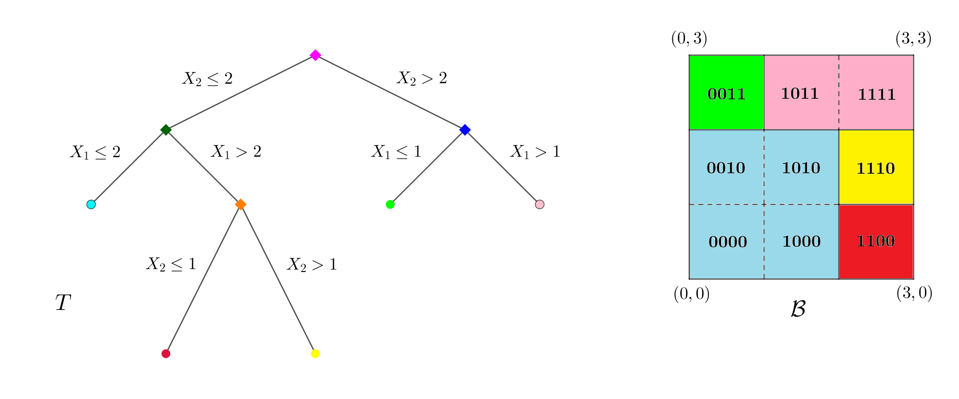
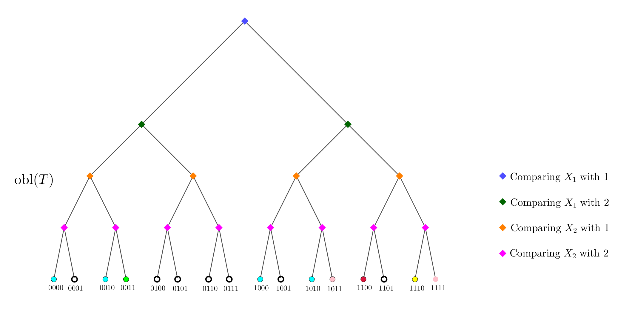
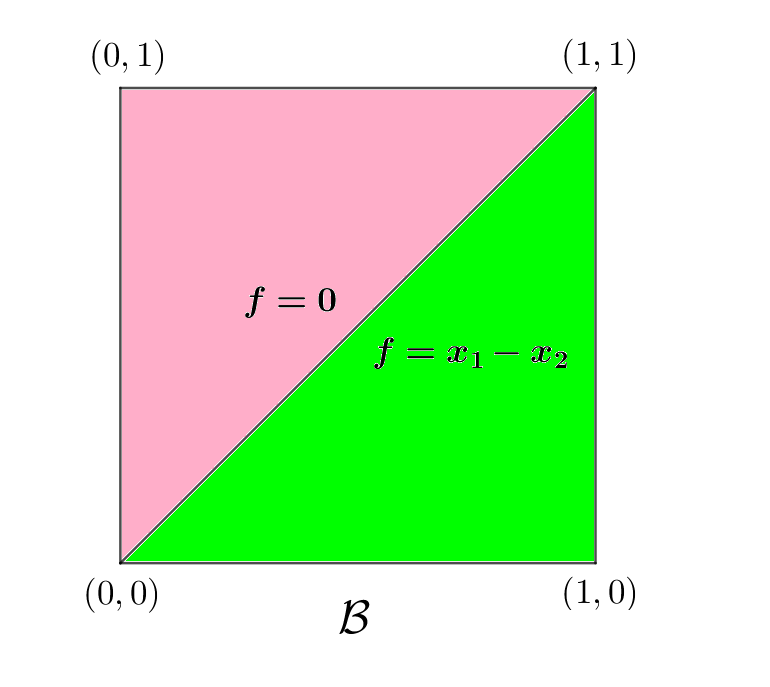
Appendix G A remark on non-oblivious trees
In this short appendix, we point out that Theorem 3.6 can be utilized to explicitly compute marginal game values such as Shapley or Banzhaf for any decision tree .
To this end, we present a systematic method of turning a general decision tree into an oblivious decision tree with the same input-output function—a tree to which Theorem 3.6 can then be applied.
Impose an ordering on features appearing in , and then order the splits (feature,threshold) occurring in lexicographically. Next, take to be the oblivious decision tree which, throughout its level (the root being on the level), splits on the split of .
This is all illustrated in Figure 9.
Clearly, the function computed by is identical to the one that computes. But the partition determined by the former is more intricate—it is the grid completion of the partition determined by the latter.
The formula from Theorem 3.6 (or its generalizations in Appendix F)
can now be applied to to obtain marginal Shapley (or Banzhaf or Owen) values of the original tree in terms of the leaf values of and the probabilities of regions in . Nevertheless, the probabilities associated with regions that lie in
cannot be estimated directly based on leaf weights of the trained tree ; they should be
estimated separately using the training data or a background dataset (e.g. with a formula such as (3.26)). Assuming that these probabilities are provided for a non-oblivious tree , the complexity of computing the marginal Shapley value of a feature is no higher than
according to (3.18). Here, is the number of distinct features appearing in (and hence in ), and is the number of leaves of (so the number of internal nodes of , , is an upper bound for the depth of ). Hence for an ensemble of decision trees in which the number of distinct features per tree is limited, it may be feasible to compute marginal Shapley (or Banzhaf or Owen) feature attributions by applying the theory developed in Section 3.4 to the ensemble of oblivious trees.
Appendix H Comparison with ReLU networks
It is well known that a neural network with ReLU activations cuts the input space into convex polytope regions such that on each of them the computed function is linear [50].
These linear regions are determined by activation patterns, i.e. the on/off states of hidden neurons.
Deep ReLU networks often result in very complicated partitions of the space into polytopes. These partitions can moreover be utilized to study the networks’ expressive power [54].
One can immediately draw a parallel between the partition into polytope regions induced by a ReLU network and the rectangular partition of the input space that a tree-based model determines.
With respect to the partition in hand, the input-output function is piecewise linear in the case of the former and piecewise constant in the case of the latter. Indeed, it is suggested that “unwrapping” a ReLU network into its activation regions may be used for generating global feature importance values as well as creating visual aids for interpretation and diagnostic [66].
Here, we shall see that when it comes to game-theoretic local feature attributions, Theorem 3.2 for tree-based models does not carry over to ReLU networks.
Example H.1.
Suppose the predictors are supported in the unit square and consider the piecewise constant function
which is obtained from applying ReLU to a linear function. The unit square is thus cut into two triangles as in Figure 10. Suppose and admit probability density functions, and denote them by and respectively. Also denote the joint probability density function for by . Identity (2.5) yields the marginal Shapley values of the model as
| (H.1) |
The expressions above are non-linear; so a piecewise-linear ReLU model does not necessarily result in piecewise-linear marginal feature attributions. This is in contrast to the case of piecewise-constant functions computed by tree-based models where, according to Theorem 3.2, marginal feature attributions are piecewise constant. Moreover, compared to tree ensembles, the null-player axiom cannot be utilized as easily. For instance, in the example above, is constant on the triangular region but this does not mean that and are constant over that region.
The last example demonstrates some of the subtleties that emerge once one works with polytope regions arising from ReLU networks instead of rectangular regions determined by tree-based models. As a matter of fact, it easily follows from the arguments in the proof of Theorem 3.2 that if a model is piecewise constant or piecewise linear with respect to a rectangular partition of the input space, then its feature attributions are the same type of functions with respect to the grid partition . As observed in the example, this fails if is not rectangular because then the feature attributions can become completely non-linear.
Acknowledgments. The authors would like to thank Raghu Kulkarni, Patrick Hall, Kenrick Fernandes, Ashkan Golgoon and Mohammad Ahmadpoor for fruitful conversations and helpful comments. We are also grateful to the anonymous referees for their valuable feedback.
References
- [1] K. Aas, M. Jullum, and A. Løland. Explaining individual predictions when features are dependent: More accurate approximations to Shapley values. Artificial Intelligence, 298:103502, 2021.
- [2] E. Al Daoud. Comparison between XGBoost, LightGBM and CatBoost using a home credit dataset. International Journal of Computer and Information Engineering, 13(1):6–10, 2019.
- [3] D. Alvarez Melis and T. Jaakkola. Towards robust interpretability with self-explaining neural networks. Advances in neural information processing systems, 31, 2018.
- [4] S. I. Amoukou, T. Salaün, and N. Brunel. Accurate Shapley values for explaining tree-based models. In International Conference on Artificial Intelligence and Statistics, pages 2448–2465. PMLR, 2022.
- [5] R. J. Aumann and J. H. Dreze. Cooperative games with coalition structures. International Journal of game theory, 3(4):217–237, 1974.
- [6] J. F. Banzhaf III. Weighted voting doesn’t work: A mathematical analysis. Rutgers L. Rev., 19:317, 1964.
- [7] L. Breiman. Random forests. Machine learning, 45(1):5–32, 2001.
- [8] T. W. Campbell, H. Roder, R. W. Georgantas III, and J. Roder. Exact Shapley values for local and model-true explanations of decision tree ensembles. Machine Learning with Applications, page 100345, 2022.
- [9] R. Caruana and A. Niculescu-Mizil. An empirical comparison of supervised learning algorithms. In Proceedings of the 23rd international conference on Machine learning, pages 161–168, 2006.
- [10] H. Chen, I. C. Covert, S. M. Lundberg, and S.-I. Lee. Algorithms to estimate Shapley value feature attributions. arXiv e-prints, page arXiv:2207.07605v1, July 2022.
- [11] H. Chen, J. D. Janizek, S. Lundberg, and S.-I. Lee. True to the Model or True to the Data? arXiv e-prints, page arXiv:2006.16234, June 2020.
- [12] H. Chen, S. Lundberg, and S.-I. Lee. Explaining models by propagating Shapley values of local components. Explainable AI in Healthcare and Medicine: Building a Culture of Transparency and Accountability, pages 261–270, 2021.
- [13] T. Chen and C. Guestrin. XGBoost: A scalable tree boosting system. In Proceedings of the 22nd acm sigkdd international conference on knowledge discovery and data mining, pages 785–794, 2016.
- [14] A. Chopra and P. Bhilare. Application of ensemble models in credit scoring models. Business Perspectives and Research, 6(2):129–141, 2018.
- [15] A. Datta, S. Sen, and Y. Zick. Algorithmic transparency via quantitative input influence: Theory and experiments with learning systems. In 2016 IEEE symposium on security and privacy (SP), pages 598–617. IEEE, 2016.
- [16] T. G. Dietterich. Ensemble methods in machine learning. In International workshop on multiple classifier systems, pages 1–15. Springer, 2000.
- [17] Documentation. CatBoost https://catboost.ai/en/docs.
- [18] Documentation. LightGBM https://lightgbm.readthedocs.io/en/latest/index.html.
- [19] Documentation. TreeSHAP https://shap-lrjball.readthedocs.io/en/latest/generated/shap.TreeExplainer.html.
- [20] Documentation. XGBoost https://xgboost.readthedocs.io/en/stable.
- [21] A. Dorogush, V. Ershov, and A. Gulin. CatBoost: gradient boosting with categorical features support. arXiv e-prints, page arXiv:1810.11363, Oct. 2018.
- [22] ECOA. Equal Credit Opportunity Act https://www.justice.gov/crt/equal-credit-opportunity-act-3.
- [23] K. Fernandes, P. Vinagre, P. Cortez, and P. Sernadela. Online News Popularity. UCI Machine Learning Repository, 2015. DOI: 10.24432/C5NS3V.
- [24] M. Ferov and M. Modrý. Enhancing LambdaMART Using Oblivious Trees. arXiv e-prints, page arXiv:1609.05610, Sept. 2016.
- [25] FHA. Fair Housing Act https://www.justice.gov/crt/fair-housing-act-1.
- [26] J. H. Friedman. Greedy function approximation: a gradient boosting machine. Annals of statistics, pages 1189–1232, 2001.
- [27] L. Grinsztajn, E. Oyallon, and G. Varoquaux. Why do tree-based models still outperform deep learning on typical tabular data? In Thirty-sixth Conference on Neural Information Processing Systems Datasets and Benchmarks Track, 2022.
- [28] K. Hamidieh. Superconductivty Data. UCI Machine Learning Repository, 2018. DOI: 10.24432/C53P47.
- [29] J. T. Hancock and T. M. Khoshgoftaar. CatBoost for big data: an interdisciplinary review. Journal of big data, 7(1):1–45, 2020.
- [30] T. Hastie, R. Tibshirani, J. H. Friedman, and J. H. Friedman. The elements of statistical learning: data mining, inference, and prediction, volume 2. Springer, 2009.
- [31] X. He, J. Pan, O. Jin, T. Xu, B. Liu, T. Xu, Y. Shi, A. Atallah, R. Herbrich, S. Bowers, et al. Practical lessons from predicting clicks on ads at Facebook. In Proceedings of the eighth international workshop on data mining for online advertising, pages 1–9, 2014.
- [32] L. Hu, J. Chen, J. Vaughan, S. Aramideh, H. Yang, K. Wang, A. Sudjianto, and V. N. Nair. Supervised machine learning techniques: An overview with applications to banking. International Statistical Review, 89(3):573–604, 2021.
- [33] D. Janzing, L. Minorics, and P. Blöbaum. Feature relevance quantification in explainable AI: A causal problem. In International Conference on artificial intelligence and statistics, pages 2907–2916. PMLR, 2020.
- [34] B. John. When to Choose CatBoost Over XGBoost or LightGBM [Practical Guide] (neptun.ai), 2022.
- [35] M. Jullum, A. Redelmeier, and K. Aas. groupShapley: Efficient prediction explanation with Shapley values for feature groups. arXiv e-prints, page arXiv:2106.12228, June 2021.
- [36] U. Kamath and J. Liu. Explainable Artificial Intelligence: An Introduction to Interpretable Machine Learning. Springer, 2021.
- [37] Y. Kamijo. A two-step Shapley value for cooperative games with coalition structures. International Game Theory Review, 11(02):207–214, 2009.
- [38] A. Karczmarz, T. Michalak, A. Mukherjee, P. Sankowski, and P. Wygocki. Improved feature importance computation for tree models based on the Banzhaf value. In The 38th Conference on Uncertainty in Artificial Intelligence, 2022.
- [39] G. Ke, Q. Meng, T. Finley, T. Wang, W. Chen, W. Ma, Q. Ye, and T.-Y. Liu. LightGBM: A highly efficient gradient boosting decision tree. Advances in neural information processing systems, 30, 2017.
- [40] L. Koralov and Y. Sinai. In Theory of Probability and Random Processes. Springer, 2007.
- [41] K. Kotsiopoulos, A. Miroshnikov, K. Filom, and A. R. Kannan. Approximation of group explainers with coalition structure using Monte Carlo sampling on the product space of coalitions and features. arXiv e-prints, page arXiv:2303.10216, Mar. 2023.
- [42] H. Lakkaraju, E. Kamar, R. Caruana, and J. Leskovec. Interpretable & Explorable Approximations of Black Box Models. arXiv e-prints, page arXiv:1707.01154, July 2017.
- [43] Y. Lou, R. Caruana, J. Gehrke, and G. Hooker. Accurate intelligible models with pairwise interactions. In Proceedings of the 19th ACM SIGKDD international conference on Knowledge discovery and data mining, pages 623–631, 2013.
- [44] S. M. Lundberg, G. Erion, H. Chen, A. DeGrave, J. M. Prutkin, B. Nair, R. Katz, J. Himmelfarb, N. Bansal, and S.-I. Lee. From local explanations to global understanding with explainable AI for trees. Nature machine intelligence, 2(1):56–67, 2020.
- [45] S. M. Lundberg, G. G. Erion, and S.-I. Lee. Consistent Individualized Feature Attribution for Tree Ensembles. arXiv e-prints, page arXiv:1802.03888, Feb. 2018.
- [46] S. M. Lundberg and S.-I. Lee. A unified approach to interpreting model predictions. Advances in neural information processing systems, 30, 2017.
- [47] L. Merrick and A. Taly. The explanation game: Explaining machine learning models using Shapley values. In International Cross-Domain Conference for Machine Learning and Knowledge Extraction, pages 17–38. Springer, 2020.
- [48] A. Miroshnikov, K. Kotsiopoulos, K. Filom, and A. R. Kannan. Stability theory of game-theoretic group feature explanations for machine learning models. arXiv e-prints, page arXiv:2102.10878v5, Feb. 2021.
- [49] C. Molnar. Interpretable machine learning. Lulu.com, 2020.
- [50] G. F. Montufar, R. Pascanu, K. Cho, and Y. Bengio. On the number of linear regions of deep neural networks. Advances in neural information processing systems, 27, 2014.
- [51] A. Nahon. XGBoost, LightGBM or CatBoost — which boosting algorithm should I use? (medium.com/riskified-technology), 2019.
- [52] H. Nori, S. Jenkins, P. Koch, and R. Caruana. InterpretML: A Unified Framework for Machine Learning Interpretability. arXiv e-prints, page arXiv:1909.09223, Sept. 2019.
- [53] G. Owen. Values of games with a priori unions. In Mathematical economics and game theory, pages 76–88. Springer, 1977.
- [54] M. Raghu, B. Poole, J. Kleinberg, S. Ganguli, and J. Sohl-Dickstein. On the expressive power of deep neural networks. In international conference on machine learning, pages 2847–2854. PMLR, 2017.
- [55] Y. A. Reshef, D. N. Reshef, H. K. Finucane, P. C. Sabeti, and M. Mitzenmacher. Measuring dependence powerfully and equitably. ArXiv, abs/1505.02213, 2015.
- [56] M. T. Ribeiro, S. Singh, and C. Guestrin. "Why should I trust you?" Explaining the predictions of any classifier. In Proceedings of the 22nd ACM SIGKDD international conference on knowledge discovery and data mining, pages 1135–1144, 2016.
- [57] M. T. Ribeiro, S. Singh, and C. Guestrin. Anchors: High-precision model-agnostic explanations. In Proceedings of the AAAI conference on artificial intelligence, volume 32, 2018.
- [58] B. P. Roe, H.-J. Yang, J. Zhu, Y. Liu, I. Stancu, and G. McGregor. Boosted decision trees as an alternative to artificial neural networks for particle identification. Nuclear Instruments and Methods in Physics Research Section A: Accelerators, Spectrometers, Detectors and Associated Equipment, 543(2-3):577–584, 2005.
- [59] C. Rudin. Stop explaining black box machine learning models for high stakes decisions and use interpretable models instead. Nature Machine Intelligence, 1(5):206–215, 2019.
- [60] A. Saabas. treeinterpreter python package https://github.com/andosa/treeinterpreter, 2019.
- [61] S. Saha. XGBoost vs LightGBM: How Are They Different (neptun.ai), 2022.
- [62] L. S. Shapley. A value for n-person games, Contributions to the Theory of Games, 2, 307–317, 1953.
- [63] Y. Shuo Tan, C. Singh, K. Nasseri, A. Agarwal, and B. Yu. Fast Interpretable Greedy-Tree Sums (FIGS). arXiv e-prints, page arXiv:2201.11931, Jan. 2022.
- [64] R. Shwartz-Ziv and A. Armon. Tabular data: Deep learning is not all you need. Information Fusion, 81:84–90, 2022.
- [65] E. Štrumbelj and I. Kononenko. Explaining prediction models and individual predictions with feature contributions. Knowledge and information systems, 41(3):647–665, 2014.
- [66] A. Sudjianto, W. Knauth, R. Singh, Z. Yang, and A. Zhang. Unwrapping The Black Box of Deep ReLU Networks: Interpretability, Diagnostics, and Simplification. arXiv e-prints, page arXiv:2011.04041, Nov. 2020.
- [67] A. Sudjianto and A. Zhang. Designing Inherently Interpretable Machine Learning Models. arXiv e-prints, page arXiv:2111.01743, Nov. 2021.
- [68] M. Sundararajan and A. Najmi. The many Shapley values for model explanation. In International conference on machine learning, pages 9269–9278. PMLR, 2020.
- [69] M. Sundararajan, A. Taly, and Q. Yan. Axiomatic attribution for deep networks. In International conference on machine learning, pages 3319–3328. PMLR, 2017.
- [70] L. Torgo and R. Camacho. Ailerons Data. OpenML Data Repository, 2014.
- [71] L. Turgeman and J. H. May. A mixed-ensemble model for hospital readmission. Artificial intelligence in medicine, 72:72–82, 2016.
- [72] J. Vaughan, A. Sudjianto, E. Brahimi, J. Chen, and V. N. Nair. Explainable Neural Networks based on Additive Index Models. arXiv e-prints, page arXiv:1806.01933, June 2018.
- [73] D. Whiteson. HIGGS. UCI Machine Learning Repository, 2014. DOI: 10.24432/C5V312.
- [74] Q. Wu, C. J. Burges, K. M. Svore, and J. Gao. Adapting boosting for information retrieval measures. Information Retrieval, 13(3):254–270, 2010.
- [75] J. Yang. Fast TreeSHAP: Accelerating SHAP Value Computation for Trees. arXiv e-prints, page arXiv:2109.09847, Sept. 2021.
- [76] Z. Yang, A. Zhang, and A. Sudjianto. Enhancing explainability of neural networks through architecture constraints. IEEE Transactions on Neural Networks and Learning Systems, 32(6):2610–2621, 2020.
- [77] Z. Yang, A. Zhang, and A. Sudjianto. GAMI-Net: An explainable neural network based on generalized additive models with structured interactions. Pattern Recognition, 120:108192, 2021.
- [78] H. P. Young. Monotonic solutions of cooperative games. International Journal of Game Theory, 14(2):65–72, 1985.
- [79] Z. Zhang, Y. Zhao, A. Canes, D. Steinberg, O. Lyashevska, et al. Predictive analytics with gradient boosting in clinical medicine. Annals of translational medicine, 7(7), 2019.
- [80] W. Zhao, R. Singh, T. Joshi, A. Sudjianto, and V. N. Nair. Self-interpretable Convolutional Neural Networks for Text Classification. arXiv e-prints, page arXiv:2105.08589, May 2021.