Channel Estimation for BIOS-Assisted Multi-User MIMO Systems: A Heterogeneous Two-timescale Strategy
Abstract
Bilayer intelligent omni-surface (BIOS) has recently attracted increasing attention due to its capability of independent beamforming on both reflection and refraction sides. However, its specific bilayer structure makes the channel estimation problem more challenging than the conventional intelligent reflecting surface (IRS) or intelligent omni-surface (IOS). In this paper, we investigate the channel estimation problem in the BIOS-assisted multi-user multiple-input multiple-output system. We find that in contrast to the IRS or IOS, where the forms of the cascaded channels of all user equipments (UEs) are the same, in the BIOS, those of the UEs on the reflection side are different from those on the refraction side, which is referred to as the heterogeneous channel property. By exploiting it along with the two-timescale and sparsity properties of channels and applying the manifold optimization method, we propose an efficient channel estimation scheme to reduce the training overhead in the BIOS-assisted system. Moreover, we investigate the joint optimization of base station digital beamforming and BIOS passive analog beamforming. Simulation results show that the proposed estimation scheme can significantly reduce the training overhead with competitive estimation quality, and thus keeps the performance advantage of BIOS over IRS and IOS with imperfect channel state information.
Index Terms:
Channel estimation, reconfigurable intelligent surface, bilayer-intelligent omni-surface, heterogeneous two-timescale strategy, manifold optimization.I Introduction
Recently, reconfigurable intelligent surface (RIS) has provoked increasing attention in the evolution towards 6G communication, as it can enhance the cell coverage, provide virtual direct paths between the base station (BS) and user equipments (UEs), etc., by reconfiguring the radio propagation environment with limited hardware costs and power consumption [1]. Typically, RIS is a passive metasurface composed of massive reconfigurable scattering elements that can control the response of impinging signals by dynamically changing the phase shift of each element so that the communication channel can be improved with specific design objectives [2][3][4].
Most of the existing works focused on the intelligent reflecting surface (IRS), a type of RIS which can only reflect the incident signal back to the same side [5], as shown in Fig. 1(a). To overcome this topological constraint of IRS, a novel RIS named as intelligent omni-surface (IOS) or simultaneous transmitting and reflecting RIS (STAR-RIS) has been recently proposed to extend the coverage of the surface to the full-space [6][7]11 1 For the convenience of description, we refer to both IOS and STAR-RIS as IOS in this paper.. Specifically, as shown in Fig. 1(b), the signal impinging on the IOS will be split into two parts, with one part reflected to the UEs on the same side of the incident signal (referred to as UEfles), and the other part refracted to the UEs on the opposite side (referred to as UEfras). Due to this unique functionality, IOS can significantly improve the performance of UEs in the whole space, and thus be employed in various communication systems such as multiple-input multiple-output (MIMO) communication [8], non-orthogonal multiple access communication [9][10], unmanned aerial vehicle communication [11][12], etc. Meanwhile, several IOS prototypes have also been reported recently, verifying the feasibility of employing IOS in practical communication systems [13][14].
Despite of the dual functionality of reflection and refraction, the beamforming on both sides of IOS cannot be independently controlled due to the coupled phase shift for reflection and refraction signals [14][15]. Specifically, in a typical case of IOS, the phase shifts for reflection and refraction signals are just the same [6]. As shown in Fig. 1(b), this setup implies that the beamforming on both sides of the metasurface will be symmetric. Thus, if the UEs are randomly located in the cell, some beams are very likely not to be directed to any UE, so their power is wasted. To deal with this problem, in [16], we proposed a promising bilayer intelligent omni-surface (BIOS) structure with two neighbouring IOS layers (referred to as IOS1 and IOS2), which can flexibly control the beams on both sides of the surface, as shown in Fig. 1(c). Owing to this unique capability, BIOS can provide higher data rate than IRS and IOS in multi-user systems.

For all of the RIS types mentioned above, the acquisition of accurate channel state information (CSI) is crucial for the beamforming optimization. However, the channel estimation of RIS systems is a difficult task in practice, as all of the scattering elements are passive components without any ability of baseband signal processing. To address this issue, several RIS channel estimation schemes have been proposed in recent works. For IRS, which is the most popular type of RIS, a channel estimation scheme based on the least squares (LS) criterion for IRS-assisted single-user multiple-input single-output (MISO) systems has been proposed in [17], where the BS is assumed to have no prior knowledge about the channels, and thus requires high training overhead. To tackle this issue, several channel estimation approaches for reducing the overhead have been proposed by exploiting the properties of IRS channels. In particular, by utilizing the channel sparsity, several compressive sensing (CS) methods have been applied in the IRS channel estimation, e.g., orthogonal matching pursuit (OMP) [18][19], approximate message passing (AMP) [20], atomic norm minimization (ANM) [21][22], etc. Meanwhile, the property that all UEs share the same IRS-BS channel has also been exploited in some previous works to reduce the training overhead of channel estimation in IRS-assisted systems. For example, in [23], an iterative channel estimation scheme was proposed by exploiting the fact that the sparse cascaded channels of all UEs have a common row-column-block sparsity. The authors in [24] utilized the correlation between UEs’ reflected channels, and proposed a three-phase channel estimation scheme for an IRS-assisted multi-user MISO system. Furthermore, by reforming the received pilots as a tensor, two parallel factor based channel estimation algorithms were developed in [25], where the UE-IRS channels and the common IRS-BS channel are separately estimated. Another important idea to reduce the training overhead in IRS channel estimation is to utilize the channel variation property. By exploiting the fact that the coherence time periods of the IRS-BS and UE-IRS channels are different, the authors in [26] proposed a two-timescale channel estimation scheme to separately estimate the IRS-BS and UE-IRS channels in different timescales. In addition, a three-stage estimation scheme was proposed in [27] for an IRS-assisted multi-user MIMO system, where the angles of departure (AoDs) and angles of arrival (AoAs) of channels are assumed to remain unchanged for several coherence blocks, so that only the channel gains need to be updated in these blocks.
Different from the abundant research in IRS-assisted systems, so far there has been very little research on the channel estimation in IOS-assisted systems. In [28], an LS based channel estimation scheme was proposed for the IOS-assisted system working in the time switching and energy splitting model. For the BIOS-assisted system, as there are two IOSs deployed, the channel estimation problem becomes more challenging than that in the IRS- and IOS-assisted systems. Taking the downlink transmission for example, for UEfles, the BS signal is directly reflected by IOS1 to them, while for UEfras, the BS signal is not only refracted by the two IOSs, but also passes through the near-field channel between the two IOSs.
In this paper, we investigate the uplink channel estimation problem in the BIOS-assisted multi-user MIMO system, and propose a channel estimation scheme which can reduce the training overhead by exploiting the BIOS channel properties. To the best of our knowledge, this is the first attempt to tackle the channel estimation of the BIOS-assisted system. The main contributions of this work are summarized below:
- •
We investigate the equivalent baseband signal model of the BIOS-assisted system, and show that in contrast to the conventional IRS- and IOS-assisted systems, where the cascaded channels of all UEs have similar forms regardless of their locations, in the BIOS-assisted system the cascaded channels of UEfles and those of UEfras have different forms, which we refer to as the unique heterogeneous property. It is this property that makes the channel estimation in the BIOS-assisted system more difficult to deal with.
- •
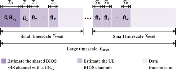
By exploiting the heterogeneous and two-timescale (HTT) properties of the BIOS channels and applying the manifold optimization (MO) method, we propose the HTT-MO channel estimation scheme. Specifically, the common BIOS-BS channel among UEs is firstly estimated over a large timescale according to the uplink pilots from a UEfra rather than a UEfle. With the estimated BIOS-BS channel, the UE-BIOS channels of all UEs are then estimated in each small timescale separately. In either the large or small timescale estimation, an MO channel estimation (MO-CE) algorithm is proposed to reduce the training overhead by exploiting the low-rank property and angle sparsity of channels.
- •
With the estimated CSI, we propose a joint BS digital and BIOS analog passive beamforming optimization algorithm aiming at maximizing the downlink sum rate of the BIOS-assisted system. The original sum rate maximization problem is first converted to an equivalent weighted mean square error minimization (WMMSE) problem, and then solved by using the alternating optimization and the coordinate descent (CD) algorithm.
- •
We provide various simulation results to verify the effectiveness of the proposed HTT-MO channel estimation scheme and the WMMSE-CD beamforming scheme, and show that although the channel estimation problem in the BIOS-assisted system is much more complicated than that in the conventional IRS- and IOS-assisted systems, the superiority in the sum rate performance of BIOS over IRS and IOS still holds for the situation with estimated CSI, thanks to the efficient utilization of the channel properties via the proposed HTT-MO scheme.
The rest of this paper is organized as follows. Section II introduces the basic structure of BIOS. Section III presents the system model and channel model of the BIOS-assisted multi-user MIMO system. Section IV presents the HTT channel estimation strategy. Section V proposes the HTT-MO channel estimation scheme, where the detailed estimation algorithms in both the large and small timescales are discussed. Section VI proposes the WMMSE-CD scheme for the beamforming optimization in the BIOS-assisted system. Simulation results are provided in Section VII. Finally, Section VIII draws the conclusions of this paper.
Notations: In this paper, the imaginary unit is denoted by . the bold lowercase letter and bold captital letter represent a column vector and a matrix, respectively. represents the -th element of , and represents the -th element of . , and denote the transpose, conjugate transpose and conjugate operators, respectively. , and denote the trace, rank and vectorization of a matrix, respectively. denotes the Frobenius norm of a matrix, while denotes the -norm of a vector. denotes the determinant (module) of a matrix (complex variable). denotes the real part of a scalar. is the expectation operator. , and denotes Hadamard, Khatri-Rao and Kronecker products, respectively. denotes a diagonal matrix with the elements of on its main diagonal, and is the extraction of the diagonal of . denotes a block diagonal matrix whose diagonal components are . denotes the circularly symmetric complex Gaussian distribution with zero mean and covariance matrix .
II Bilayer Intelligent Omni-Surface
As we mentioned in Section I, conventional RISs, like IRS and IOS, have several limitations in the beamforming design for multi-user systems. To overcome these limitations, we have proposed a novel RIS, BIOS, in [16], which consists of two neighboring layers of IOSs, as shown in Fig. 1(c). The IOS1 is set in the simultaneous reflection and refraction mode, while the IOS2 is set in the full penetration mode, which transmits the signal impinging on one side of it completely to the other side. Thereby, the incident signal will be split into two parts after passing through the BIOS. One is directly reflected by IOS1 to UEfles, and the other one is transmitted by IOS1 to IOS2, and then is refracted by IOS2 to UEfras. This unique property bestows the BIOS the degree of freedom to flexibly control the beamforming on both sides of the surface. In this paper, we assume that IOS1 and IOS2 are both uniform square planar arrays (UPAs) with a size of . Then, the effective coefficient matrices of BIOS for the downlink reflection and refraction signals can be expressed as
| (1) |
where and are the downlink diagonal coefficient matrices of IOS1 and IOS2, respectively, with . is a constant to quantify the ratio of reflection signal power to the total power of IOS1, while is the ratio of the refraction signal power. is the near field channel matrix between IOS1 and IOS2, the () element of which can be denoted by [16][29]
| (2) |
where is the size of IOS elements and is the distance between the -th element of IOS1 and the -th element of IOS2 after deployment. is the normalized power radiation pattern of IOS elements [29], and (), () are the elevation (azimuth) AoD and AoA of the channel between the -th element of IOS1 and the -th element of IOS2. Considering that is determined only by the distance between IOS1 and IOS2, which remains unchanged after the deployment of BIOS, in this paper we assume that is known to the BS.
III System Model and Channel Model
III-A System Model

As shown in Fig. 2, we consider the uplink channel estimation in a BIOS-assisted narrowband multi-user MIMO system operating in the time division duplex (TDD) mode, where a BS with isotropic antennas serves totally UEs equipped with isotropic antennas. As the direct links between the BS and UEs are assumed to be blocked, a BIOS is deployed to establish the virtual line-of-sight (LoS) paths for UEs. As mentioned in Section II, both layers of BIOS are assumed to be UPAs consisting of reconfigurable elements. UEs are divided into two groups based on their positions relative to the BIOS, with UEs located on the reflection side, indexed by , and UEs located on the refraction side, indexed by . In this work, we assume that the information of whether a UE is a UEfle or a UEfra is known to the BS. In order to simplify the channel estimation process and avoid the interference between pilots sent by UEs, it is assumed that the UEs send their pilots one-by-one to the BS over consecutive time. Taking the -th UE for example, the equivalent baseband received signal at the BS can be represented by
| (3) |
where is the -th pilot vector with the normalized power constraint and represents the additive Gaussian noise satisfying . when , and when . and are the uplink effective coefficient matrices of BIOS, with , denoting the uplink diagonal coefficient matrices of IOS1 and IOS2 for the -th pilot vector. Finally, denotes the IOS1-BS channel, and denotes the -th -IOS1 (-th -IOS2) channel for ().
III-B Cascaded Channel in the BIOS-assisted System
Normally, for the IRS/IOS-assisted systems, the received signal at the BS can be represented as a function of the cascaded channel of the IRS(IOS)-BS and the UE-IRS(IOS) channels for the convenience of channel estimation and beamforming design [30]. It can be found that in the IRS/IOS-assisted systems, the forms of the cascaded channels of all UEs are the same. However, in the BIOS-assisted system, this is not the case. In particular, for UEfles, as the is a diagonal matrix, the cascaded channel can be expressed as the Khatri-Rao product of and , which is similar to that in the IRS/IOS-assisted MIMO system [6][21][25]. Then, (3) can be represented as
| (4) |
for , where , and . (4) follows from the facts that and for any matrices , and , and diagonal matrix with .
For UEfras, however, is a matrix without any zero element. Thus, (3) can be rewritten as
| (5) |
for , where the cascaded channel . By comparing (4) and (5), it can be found that the forms of cascaded channels in the BS received signals are different for UEfles and UEfras in the BIOS-assisted system, i.e., for UEfles and and UEfras. This characteristic is referred to as the heterogeneous property, which makes the channel estimation in the BIOS-assisted system more challenging. It should also be noticed that due to the heterogeneous property, the number of matrix elements in () is times of that in (), which implies that more training overhead is required for the estimation of .
III-C Channel Model
We assume that both the BS and UEs are equipped with uniform linear array (ULA) antennas. By utilizing the Saleh-Valenzuela model [23] to characterize the propagation environment, for the -th UE, the BIOS-BS and UE-BIOS channel matrices can be expressed as
| (6) |
where and denote the number of the paths of the BIOS-BS and UE-BIOS channels, respectively, which are assumed to be known by the BS. For the BIOS-BS channel, , and represent the complex gain, the AoA and the elevation (azimuth) AoD of the -th path. For the UE-BIOS channel, similarly, , and represent the complex gain, the elevation (azimuth) AoA and the AoD of the -th path. () denotes the IOS normalized power radiation pattern of the -th (-th) path of the BIOS-BS (UE-BIOS) channel. In addition, , and denote the array response vectors of the BS, BIOS and UE, respectively. Specifically, by assuming that the arrays at the BS and UEs are half-wavelength spaced ULAs and defining
| (7) |
the corresponding array response vectors of the BS and UEs can be expressed as [23]
| (8) |
For the half-wavelength spaced UPAs at BIOS, the array response vector can be given as follows
| (9) |
where and denote the elevation and azimuth AoD or AoA of the BIOS, respectively.
III-D Sparsity of Channels in the Angle Domain
As mentioned in Section III-C, there are only a few propagation paths along the UE-BIOS-BS links due to the severe path loss and blocking effects. Thus, the BIOS-BS and UE-BIOS channels can be further transformed into an angular sparse representation as follows [23]:
| (10) |
where , and are the overcomplete angular domain dictionaries with the angle resolutions of , and , respectively. Each column of the dictionaries corresponds to one specific AoA/AoD at the BS, BIOS or the -th UE. and are the angular domain sparse matrices of and , which consist of and non-zero elements respectively corresponding to the channel path gains. By selecting the codewords from the uniform grid, and can be expressed as
| (11) |
where and . By setting and to be the angular resolutions of the BIOS along the x-axis and y-axis, can be exhibited in a similar way as , where
| (12) |
with , and .
IV Heterogeneous Two-timescale Channel Estimation Strategy
As we mentioned in Section III, the number of coefficients in the cascaded channels is huge, especially for , which leads to prohibitive training overhead if we directly estimate the cascaded channels of all UEs. In this section, we propose an HTT channel estimation strategy to reduce the requested training overhead by exploiting the channel properties in the BIOS-assisted system.
IV-A The Two-timescale Property
It can be observed that in a BIOS-assisted system, the time variation of the BIOS-BS channel and that of the UE-BIOS channel are in different scales. In particular, on one hand, as the BS and BIOS are rarely moved after deployment, the BIOS-BS channel , which is shared by all UEs, can be regarded as unchanged for a long period of time. On the other hand, the UE-BIOS channel varies in a much smaller timescale, since the movement of UEs frequently changes the propagation geometry between UEs and BIOS [26]. This two-timescale property allows the BS to only estimate once in the large timescale, and with the estimated , then can be further estimated in the small timescale. Thus, the training overhead can be significantly reduced.
However, the main difficulty is how to estimate , as the scattering elements in the BIOS-assisted system (and also the conventional RIS systems) are passive components without any capability of baseband processing. To deal with this difficulty, the authors in [26] proposed a dual-link pilot transmission scheme for the IRS-assisted system, where the full-duplex BS estimates the BS-IRS channel by firstly sending pilots to the IRS through the downlink channel, and then receiving the reflected signals from the IRS via the uplink channel. Although this scheme provides a way to estimate the BS-IRS channel matrix, the requirement of full duplex mode places high demands on the BS hardware. In this paper, we show that it is possible to estimate the BIOS-BS channel without taking the full-duplex assumption, but based on the uplink pilots sent by a UE in the large timescale, and the estimated can be used for the estimation of the UE-BIOS channels of all UEs. However, to make it workable, we need to deal with the challenge of the heterogeneous property of the BIOS channels.
IV-B The Challenge of the Heterogeneous Property
As we have pointed out in Section III-B that, from (4) and (5), the signals received by the BS from the UEfles and the UEfras have different expressions of the cascaded channels, where the former is a function of and the latter is a function of . This channel heterogeneous property makes the channel estimation in the BIOS-assisted system more challenging, especially when taking the two-timescale property to reduce the training overhead. Taking a UEfle for example and even assuming that there is no noise effect in the channel estimation, the best channel estimates the BS can obtain, denoted by and , are not exactly and , but belong to a set satisfying the condition of . Similarly, for a UEfra, the best channel estimates belong to a set satisfying . Obviously due to the heterogeneous property, these two sets are different. However, in the two-timescale strategy, needs to be estimated first and used for the estimation of of all UEs. Thus, a workable channel estimation scheme must be the one that can make belong to both sets or at least their subsets. The following lemmas provide detailed mathematical proofs.
Lemma 1
If there is no noise effect in the channel estimation, the channel estimates and should belong to one of the following two sets depending on whether the UE is a UEfle or a UEfra
| (13) |
| (14) |
which can be further proved to be equal to the following forms respectively
| (15) |
| (16) |
where , .
Proof: (13) and (14) can be directly proved from the definitions of the cascaded channels in (4) and (5), and the proofs of (15) and (16) can be found in Appendix A.
As can be observed in the Lemma 1, for UEfles, each column of the channel estimate can differ from the corresponding column of the true channel matrix with a distinct non-zero coefficient. However, for UEfras, these non-zero coefficients should be identical for all columns, which means the feasible set of for UEfras is a subset of that for UEfles. Thus, it can be shown in the following lemma that, to implement the two-timescale strategy in the BIOS-assisted system, if a UE is selected to send pilots for the BS to estimate in the large timescale and then use the result to estimate of all UEs in the small timescale, such a UE should be a UEfra rather than a UEfle due to the heterogeneous property.
Lemma 2
If a UEfra is chosen to send pilots to the BS for the estimation of in the large timescale and is defined as the estimation result with no noise effect, then for UEfras, belongs to , while for UEfles, belongs to a subset of with , where is the estimation result in the small timescale with no noise effect.
However, if a UEfle is chosen to send pilots in the large timescale, then for UEfras, the resulting does not belong to , which means that the accurate CSI for UEfras cannot be achieved even when there is no noise effect.
Proof: To prove the first part of this lemma, if a UEfra is chosen to send pilots to the BS for the estimation of the true channel in the large timescale, then can be expressed as according to (16). With , the BS can estimate UE-by-UE in the small timescale, based on its received pilots sent from UEs, and the estimation result for all UEs should satisfy according to (15) and (16). Then, it can be seen that for UEfras, belongs to , while for UEfles, is in a subset of with .
To prove the second part, if a UEfle is chosen to send pilots for the estimation of in the large timescale, the resulting can be represented as according to (15), where is a distinct coefficient for each column. However, based on this , in the small timescale, for UEfras, the BS cannot find a channel estimate so that , i.e., , since according to (16) but .
IV-C HTT Channel Estimation Strategy
With the two-timescale and heterogeneous properties of the BIOS channels discussed above, we come up to the HTT channel estimation strategy, which is also depicted in Fig. 3. At first, the BS estimates the BIOS-BS channel over a large timescale based on the uplink pilots sent by a selected UEfra, e.g., the -th UE. Then, in the small timescale, the BS estimates the UE-BIOS channel for each UE based on the received uplink pilots and its estimated channel matrix in the large timescale. It can be found that in the large timescale, there are a total of coefficients need to be estimated for and , while in the small timescale, there are a total of coefficients in for all UEs. In comparison, in the conventional cascaded channel estimation strategy, the BS needs to estimate the cascaded channel for each UE, and thus the total number of coefficients need to be estimated is . Comparing these two numbers, it can be seen that the HTT channel estimation strategy can significantly reduce the number of coefficients to be estimated and in turn the training overhead.
V HTT-MO Channel Estimation Scheme
In this section, based on the proposed HTT channel estimation strategy, we exploit the channel sparsity to further reduce the pilot overhead, and design the HTT-MO scheme for the channel estimation in the BIOS-assisted system.
V-A Channel Sparsity
Although the proposed HTT strategy can significantly reduce the training overhead, the channel estimation is still challenging due to the large number of antennas at both the BS and UEs, and the large number of scattering elements at the BIOS as well, which result in much training overhead. Fortunately, it can be further reduced by exploiting the channel sparsity in the angle domain shown in (10). The following two lemmas illustrate the channel sparsity of the BIOS-assisted system in detail.
Lemma 3
If and , where and denote the number of paths of the BIOS-BS and UE-BIOS channels, respectively, as defined in (6), we have
| (17) |
Proof: We take the proof of as an example. The proof of can be completed in a similar way. According to (6), the BIOS-BS channel can be rewritten as
| (18) |
where , and , with and
. As all of the column vectors of are linearly independent, we have . Similarly, we can also obtain that and . According to the
properties of Kronecker product and Khatri-Rao matrix product, we can transform into the following form
| (19) |
where and . Then, according to the rank properties of matrix [31], for arbitrary and , we have
| (20) |
By substituting (19) into (20), we have . Finally, as the rank of is also , we can further substitute (18) into (20) and obtain that .
Lemma 4
If , and , we have , , with and .
Proof: We take the proof of as an example. According to Section III-D, and are both unitary matrices as and . Therefore, can be rewritten in the form . As only consists of non-zero elements, we have .
Lemma 3 and Lemma 4 reveal the channel low-rank and angle sparse properties, respectively. Although these properties correspond to the true channel matrices and , it can be also proved that for any UE, Lemma 3 and Lemma 4 still hold for any estimated and , as according to Lemma 2, there is only a scalar difference between () and ().
V-B Estimation of in the Large Timescale
For the two-timescale strategy and according to Lemma 2, the first step at the BS is to estimate based on its received pilots sent from a UEfra, e.g., the -th UE for , in the large timescale. Based on (5), the channel estimation objective can be established similar to that of the LS problem. By further utilizing the channel sparsity properties exhibited in Lemmas 3 and 4, the estimation problem of along with can be formulated as
| (21) |
where , , and is the number of pilot vectors for the estimation of in one large timescale. It can be seen that (21) is difficult to solve due to the multiple coupled variables and the highly non-convex constraints, and thus it may not be possible to achieve a globally optimal solution. However, with some specific processing, we can rewrite the original problem and obtain a locally optimal solution of . First to deal with the -norm constraints in (21), we use the -norm regularization to relax them and rewrite (21) as
| (22) |
where and are the tuning parameters which control the contributions of the -norm. To further deal with the multiple coupled variables and , we apply the alternating minimization method and decompose (22) into the following two subproblems
| (23) |
| (24) |
Finally, to deal with the low-rank constraint in (23) and (24), it can be seen that it actually corresponds to a Riemannian manifold space, and thus the MO method [32][33] can be applied, where the optimization variable is iteratively updated in the direction of the Riemannian gradient and then is retracted back into the complex fixed-rank MO to make the result satisfy the low-rank constraint.
The crucial step is to derive the Riemannian gradient, which can be deduced from the classic conjugate gradient in the Euclidean space. By using some properties in matrix derivation such as , and , the Euclidean conjugate gradient of the objective function in (23) can be found to be given by
| (25) |
where is computed as . Similarly, the Euclidean conjugate gradient of the objective function in (24) is given by
| (26) |
where is denoted as .
With the derived Euclidean conjugate gradient, we can project it onto the tangent space to obtain the Riemannian gradient. Then, by iteratively updating the corresponding variable with the Armijo backtracking step [34] and retracting it back to the complex fixed-rank manifold, and can be alternatively estimated with the other one fixed. The overall algorithm is referred to as the MO-CE algorithm and is summarized in Algorithm 1.
V-C Estimation of for All UEs in the Small Timescale
As the BIOS-BS channel varies much slower than the UE-BIOS channels, in the small timescale, the BS can separately estimate them for all UEs over consecutive time based on its estimated BIOS-BS channel in the large timescale. Without loss of generality, we focus on the estimation of with uplink pilot vectors sent by the -th UE. Considering the channel sparsity, the estimation problem of with the LS objective similar to that in (24) is formulated as follows
| (27) |
where is given in (3), when , and when . It is worth noting that (27) is suitable for both UEfras and UEfles. As (27) has the same form as (24), it can also be solved by the MO method. It can be derived that the Euclidean gradients is given by
| (28) |
The Riemannian gradient can then be obtained by projecting the Euclidean gradient onto the tangent space. By updating the variable iteratively via the MO method until convergence, can be finally obtained.
V-D Analysis of Training Overhead
In this subsection, we analyze the training overhead of the proposed HTT-MO scheme in terms of the required number of pilot vectors and that of the conventional LS scheme. By recalling Fig. 3, we can see that the overall training overhead of the HTT-MO scheme is given by , where is the ratio of the length of a large timescale to that of a small timescale. It is worth noting in the large timescale both and need to be estimated while in the small timescale only needs to be estimated for each UE. Furthermore, as the estimation result in the large timescale must be used for the estimation of in the small timescale, the estimation accuracy of must be higher. Thus, should be larger than .
For comparison, we consider the traditional LS channel estimation scheme for the proposed BIOS-assisted system. As it does not exploit the heterogeneous, two-timescale and sparsity properties of channels, the traditional LS channel estimation scheme has to estimate the high-dimensional cascaded channels for all UEfles and UEfras in each small timescale, and thus results in prohibitive pilot overhead. To analyze the number of required pilot vectors in this traditional channel estimation scheme, we rewrite the equivalent baseband received signal of the BIOS-assisted system in (4) and (5) as follows
| (29) |
| (30) |
where (29) corresponds to UEfles, and (30) corresponds to UEfras. In this situation, the traditional LS channel estimation scheme needs to estimate the high-dimensional cascaded channels, i.e., for UEfles and for UEfras, and the corresponding number of required pilot vectors is at least and , respectively. As the cascaded channels of all UEs need to be updated in each small timescale, the total number of pilot vectors in the LS estimation scheme in a large timescale is at least , which is more than if setting , , , and . Such amount of overhead cannot be afforded in practical systems. In contrast, simulation results in Section VII will show that in the BIOS-assisted system with the same setup, only about two thousands of pilot vectors are required by the HTT-MO scheme in a large timescale.
VI WMMSE-CD Beamforming Optimization
With the estimated CSI by the HTT-MO scheme in Section V, in this section, we focus on the multi-user downlink beamforming optimization, and propose the WMMSE-CD scheme to maximize sum data rate of all UEs on both sides of the BIOS.
VI-A Problem Formulation
Assuming that the uplink and downlink channels are reciprocal, the estimated CSI of the uplink BIOS-BS and UE-BIOS channels can be utilized in the downlink beamforming optimization. Assuming that the BS sends data streams to each UE, the received signal at the -th UE, , can be represented by
| (31) |
where is the BS precoder, is the symbol vector with , and is the noise at the -th UE. Then, the effective data rate (per Hertz) of the -th UE can be expressed as
| (32) |
where denotes the efficient channel matrix from the BS to the -th UE, and denotes covariance of the noise plus multiuser interference at the -th UE. is the length of a large timescale in terms of the number of symbols within this period as shown in Fig. 3, and denotes the total training overhead in terms of the number of pilot symbols.
According to [35], the sum rate maximization (SRM) problem can be solved via an equivalent WMMSE problem. It turns out that this optimization approach can also be applied for solving the joint BS-BIOS beamforming optimization problem with the SRM objective, and the equivalent WMMSE problem is given by
| (33) |
where the first constraint represents the normalized transmit power constraint at the BS, and the second one corresponds to the constant modulus constraint of the BIOS passive scattering elements. is the mean square error (MSE) matrix of the -th UE, with denoting the combining matrix. is an auxiliary variable to establish the equivalence between the SRM problem and the WMMSE problem.
To deal with the multivariate optimization difficulty, the alternating minimization method is applied. Firstly, and are optimized while keeping other variables fixed, which can be shown to have the following closed-form solutions
| (34) |
Then, to optimize the BS precoder and the BIOS passive beamformers while keeping and fixed, by expanding the MSE matrix in (33) and removing the terms that are not related to the optimization variables, problem (33) can be simplified as
| (35) |
where , , and .
VI-B Optimization of the BS Precoder
VI-C Optimization of the IOS1
When optimizing the passive beamformer while keeping other variables fixed in (35), the difficulty is the non-convex constant modulus constraint of the scattering elements. One way to solve this difficulty is to apply the CD algorithm [36], and alternatively optimize each element of . By defining the equivalent IOS1-UEs channel as
the objective function in (35) can be represented as
| (37) |
where , and . The equality follows from the facts that , , and for arbitrary matrices , and diagonal matrix , with and . Without loss of generality, we assume that the element to be optimized in the current iteration of the CD algorithm is with other elements of fixed. Then, by omitting the constant terms irrelevant to the optimization of , the objective function can be simplified as
| (38) |
It can be shown that the optimal solution of with other elements fixed is given by
| (39) |
VI-D Optimization of the IOS2
As the performance of UEfle is not related to , we can divide in (35) into two terms, with one corresponding to the UEfras, which is related to , and the other to the UEfles, which can be taken as a constant when optimizing . By defining
, can be further reformed as
| (40) |
where , ,
, ,
and . As (40) is similar to (37), can also be optimized by the CD algorithm.
Finally, the WMMSE-CD algorithm for the BIOS-assisted multi-user MIMO system can be accomplished by alternatively optimizing , , , and . As the objective function monotonically decreases after the optimization of each variable, the WMMSE-CD algorithm is guaranteed to converge to a locally optimal solution of problem (33). It is worth noting that although we use the true channel matrices and in the derivation of WMMSE-CD algorithm, the solutions of the variables in (34), (36) and (39) still hold for the estimates and obtained by the proposed HTT-MO scheme, as there is only a scalar difference between () and () if there is no noise effect in the channel estimation.
VII Simulation Results
VII-A Simulation Setup
Consider a BIOS-assisted system where the IOS1 is set in the simultaneous reflection and refraction mode with . The number of UEs is set to , with on the reflection side and on the refraction side, i.e., , . The number of ULA elements at the BS and UEs is , and that of the UPA elements of the BIOS is with . For all of the ULAs and the two UPAs, the distance between neighboring units is , with denoting the wavelength of carrier wave. For the BIOS, the distance between the two IOSs is . For the channel model in (6), the path number of both and is set to , i.e., . Similar to that in [21][32], the first path, i.e., (), is set as the LoS path of () with its complex path gain distributed as , while other paths are NLoS paths with the path gain distribution of . For the BS and UEs, the AoAs/AoDs are assumed to be uniformly distributed in , while for the BIOS, the azimuth and elevation AoAs/AoDs are assumed to satisfy a uniform distribution in and , respectively22 2 With this setup, we can reform (12) by setting , , as , . In this situation, we still have due to the orthogonality between columns in , and thus the Lemma 4 still holds.. The elevation range is associated to the UEfles, and is associated to the UEfras. It is assumed that the BIOS-BS (UE-BIOS) channel is time invariant in a large (small) timescale, as shown in Fig. 3, and is independent for different large (small) timescale spans. The length of large (small) timescale is set to (), corresponding to a channel coherence time of () with a transmission bandwidth. The uplink training pilot-to-noise-ratio (PNR) is defined as , while the downlink transmission signal-to-noise-ratio (SNR) is defined as . For the HTT-MO scheme, all elements of and are randomly initialized from the constant modulus set {} to ensure a random quasi-omnidirectional beam pattern [37], and the elements of the pilot vector are also randomly selected from this set. All simulation results are averaged over 200 realizations.
VII-B Performance of the HTT-MO Channel Estimation Scheme
As mentioned in Section IV-B, even when there is no noise effect, the obtained and of all UEs by the proposed HTT-MO scheme is still different from the real and by a coefficient, i.e., and . Thus, it is not suitable to simply take the estimation MSE of or as a performance metric. Instead, we take the normalized MSE (NMSE) of to evaluate the performance of channel estimation, which is defined as .
We first evaluate the performance of the large timescale estimation step in the HTT-MO scheme. As introduced in Section V, a UEfra is selected for the estimation of in the large timescale estimation, and both and its UE-BIOS channel are estimated via the MO-CE algorithm. Fig. 4(a) exhibits the NMSE performance of this selected UEfra, which is defined as , for different values of PNR and training overhead . It can be seen that for small , e.g., , the proposed MO-CE algorithm suffers from a shortage of training overhead, resulting in an NMSE larger than regardless of the PNR. However, with the increase of , the performance is rapidly improved, and then reaches the gentle descent region for all PNRs.

Next, Fig. 4(b) demonstrates the average NMSE performance of all UEs in the small timescale, which is defined as , based on the obtained in the large timescale with . The PNR is set the same in both the large and small timescales. As can be observed from this figure, in this step the NMSE decreases monotonously with the increase of or PNR, which is similar to that in the large timescale estimation shown in Fig. 4(a). However, the required is much smaller than to achieve similar NMSE performance, e.g., and to reach a NMSE of when . This is mainly because in the small timescale, the BS only needs to estimate the UE-BIOS channel for each UE with the obtained , while in the large timescale, both and should be estimated for the selected UEfra. However, even if the is sufficient, the NMSE performance in the small timescale cannot exceed that in the large timescale estimation shown in Fig. 4(a), since the channel estimation performance of small timescale is limited by the estimation quality of obtained in the large timescale.
VII-C Sum Rate Performance

To further evaluate the effectiveness of the proposed HTT-MO channel estimation scheme and the WMMSE-CD beamforming scheme, Fig. 5 exhibits the sum rate performance of the BIOS-assisted system with or without channel estimation errors, represented by the solid and dashed lines, respectively. In the case with channel estimation errors, the CSI used for the beamforming is obtained by the HTT-MO scheme with . In the case without channel estimation errors, the pilot overhead is still counted and set the same as that in the case with estimation errors in order to provide a benchmark.
Fig. 5(a) shows the sum rate performance as a function of , when is fixed at . It can be seen that the sum rate performance is very poor due to the low channel estimation quality when is very insufficient (below ), and starts to increase rapidly when becomes larger. As continues to increase, however, the sum rate begins to decrease as the estimation quality cannot be significantly improved, while according to (32), the sum rate gradually decreases with more pilot overhead. In general, there is a best choice of to balance the sum rate improvement due to more accurate channel estimation quality and the data rate loss due to more pilot overhead.
Fig. 5(b) also provides the sum rate performance as a function of with . Similar to that in Fig. 5(a), the sum rate with estimated CSI first increases and then decreases with the increase of , reaching the maximum sum rate with about due to the trade-off between the estimation accuracy and the consumption of training overhead.
VII-D Comparison of the Sum Rate Performance of BIOS-, IRS- and IOS-assisted systems

In this subsection, we compare the sum rate performance of the proposed BIOS-assisted system to that of the conventional IRS- and IOS-assisted systems with both perfect CSI and estimated CSI. For the IOS-assisted system, we set to simultaneously serve UEs on both sides. The beamforming design of all these three systems are accomplished by the proposed WMMSE-CD scheme as both IRS and IOS can be regarded as a special case of BIOS.
Fig. 6(a) first depicts the sum rate performance of the BIOS-, IRS- and IOS-assisted systems versus SNR with perfect CSI, where the BS is assumed to have perfect knowledge of CSI without any pilot consumption. As can be observed, for all of the three systems, the sum rate performance increases monotonously with the SNR, while the BIOS always outperforms the IRS and IOS as it can independently control the beamforming on both sides. Meanwhile, the IRS performs the worst as it can only serve the UEs on the same side with the BS.
Next, we compare their performance with estimated CSI. For the channel estimation in the conventional IRS- and IOS-assisted systems, we adopt the following channel estimation schemes.
- •
- •
BA-LS [25]: Instead of directly estimating the cascaded channels, the authors of [25] decoupled the IRS-BS and UE-IRS channels by modeling the received pilots as a tensor, and then estimated these channels with an alternating LS algorithm for the IRS-assisted MIMO system. We extend this scheme to the IOS-assisted MIMO system in our simulation.
- •
CS-EST [32]: A three-stage scheme was proposed in [32] to estimate the cascaded channel for the IRS-assisted single-user MIMO system. The AoDs at the UE, AoAs at the BS and the cascaded channel are estimated in each stage by the OMP algorithm. In this paper, we apply this scheme in the IOS- and IRS-assisted multi-user MIMO systems by separately estimating the cascaded channels of all UEs.
Fig. 6(b) depicts the sum rate performance of the BIOS-, IRS- and IOS-assisted systems as a function of SNR with estimated CSI. The PNR is assumed to be higher than the SNR. As more training overhead provides higher estimation accuracy but occupies more transmission time, we select the best overhead for each estimation scheme and for each SNR in the sense of maximizing the sum rate of the corresponding system, instead of setting a fixed number of training pilots.
By comparing Fig. 6(b) with Fig. 6(a), we can see that all of the three systems suffer from rate reduction due to the consumption of training overhead as well as channel estimation errors. As the TS-LS scheme does not exploit any property of channels in the IRS- and IOS-assisted systems, it needs extremely high training overhead, e.g., at least pilot vectors in a small timescale, and thus reaches the smallest sum rate for both IRS- and IOS-assisted systems. For the BA-LS scheme, although it utilizes the property that all UEs share the same RIS-BS channel, the required number of training overhead is still high, e.g., at least pilot vectors in a small timescale, which significantly affects the sum rate performance of IRS- and IOS-assisted systems. By contrast, the CS-EST scheme can efficiently exploit the angle domain sparsity of channels in the IRS- and IOS-assisted systems, the required training overhead in a small timescale is only in the order of . Thus, the sum rate of both the IRS- and IOS-assisted systems with the CSI obtained by the CS-EST scheme is much higher than that with the TS-LS and BA-LS schemes. Finally, although the channel estimation in the BIOS-assisted system is much more complicated than that in the IRS- and IOS-assisted systems as we discussed in Section III and Section IV, results in this figure show that the BIOS-assisted system with the CSI obtained by the proposed HTT-MO scheme significantly outperforms the IRS- and IOS-assisted systems for medium and high SNRs. This performance advantage not only results from the ability of flexible beamforming control on both sides bestowed by the BIOS structure, but also results from the reduction of requested training overhead by efficiently exploiting the channel properties in the BIOS-assisted system, i.e., the two-timescale, heterogeneous and sparsity properties.
VIII Conclusion
In this paper, we have investigated the channel estimation problem of the uplink BIOS-assisted multi-user MIMO system. To reduce the large pilot overhead in the channel estimation of the BIOS-assisted system, we proposed the HTT-MO channel estimation scheme by efficiently exploiting the heterogeneous, two-timescale, and sparsity channel properties, in which the BS first estimates the common BIOS-BS channel with the pilots sent by a selected UEfra in a large timescale, and then uses the estimated BIOS-BS channel to estimate the UE-BIOS channels for all UEs separately in every small timescale. In each step, by exploiting the low rank property due to the channel sparsity and applying the MO method to deal with the rank constraint, the requested pilot overhead is further reduced. In addition, we have proposed the WMMSE-CD scheme for the beamforming optimization of the downlink BIOS-assisted system to maximize the UEs’ sum rate. We have provided various simulation results to demonstrate the effectiveness of the proposed channel estimation and beamforming schemes. It has been shown that compared with the conventional RISs such as IRS and IOS, the BIOS-assisted system with the CSI estimated by the proposed HTT-MO scheme has remarkable performance advantage in sum rate, not only resulted from the truth that the BIOS can provide very flexible beamforming on both sides, but also caused by the efficient utilization of the channel properties in the HTT-MO channel estimation scheme.
Appendix A Proofs of (15) and (16) in Lemma 1
The equivalence between the two forms of in (14) and (16) can be proved by showing that for any matrices , without any zero element, the necessary and sufficient condition of is: .
Necessity: If there is an , , we have with the property of Kronecker product: .
Sufficiency: , we have:
| (41) |
| (42) |
As , each element of should be equal to the corresponding element of , i.e., for any , , and . By setting , and can thus be expressed as , . Therefore, for all and , , which means that holds for all and . Thus, we have . Similarly, we can prove that , which completes the proof of sufficiency.
References
- [1] C. Pan et al., “Reconfigurable intelligent surfaces for 6G systems: Principles, applications, and research directions,” IEEE Commun. Mag., vol. 59, no. 6, pp. 14-20, Jun. 2021.
- [2] M. Di Renzo et al., “Smart radio environments empowered by reconfigurable intelligent surfaces: How it works, state of research, and the road ahead,” IEEE J. Sel. Areas Commun., vol. 38, no. 11, pp. 2450-2525, Nov. 2020.
- [3] B. Zheng, C. You, W. Mei and R. Zhang, “A survey on channel estimation and practical passive beamforming design for intelligent reflecting surface aided wireless communications,” IEEE Commun. Surveys Tuts., vol. 24, no. 2, pp. 1035-1071, 2nd Quart., 2022.
- [4] M. A. ElMossallamy, H. Zhang, L. Song, K. G. Seddik, Z. Han, and G. Y. Li, “Reconfigurable intelligent surfaces for wireless communications: Principles, challenges, and opportunities,” IEEE Trans. Cogn. Commun. Netw., vol. 6, no. 3, pp. 990-1002, Sept. 2020.
- [5] Y. Liu et al, “Reconfigurable intelligent surfaces: Principles and opportunities,” IEEE Commun. Surveys Tuts., vol. 23, no. 3, pp. 1546-1577, 3rd Quart., 2021.
- [6] S. Zhang et al., “Intelligent omni-surfaces: Ubiquitous wireless transmission by reflective-refractive metasurfaces,” IEEE Trans. Wireless Commun., vol. 21, no. 1, pp. 219-233, Jan. 2022.
- [7] X. Mu, Y. Liu, L. Guo, J. Lin, and R. Schober, “Simultaneously transmitting and reflecting (STAR) RIS aided wireless communications,” IEEE Trans. Wireless Commun., vol. 21, no. 5, pp. 3083-3098, May 2022.
- [8] H. Niu, Z. Chu, F. Zhou, P. Xiao and N. Al-Dhahir, “Weighted sum rate optimization for STAR-RIS-assisted MIMO system,” IEEE Trans. Veh. Technol., vol. 71, no. 2, pp. 2122–2127, Feb. 2022.
- [9] C. Wu, Y. Liu, X. Mu, X. Gu and O. A. Dobre, “Coverage characterization of STAR-RIS networks: NOMA and OMA,” IEEE Commun. Lett., vol. 25, no. 9, pp. 3036–3040, Sep. 2021.
- [10] J. Zuo, Y. Liu, Z. Ding, L. Song and H. V. Poor, “Joint design for simultaneously transmitting and reflecting (STAR) RIS assisted NOMA systems,” IEEE Trans. Wireless Commun., vol. 22, no. 1, pp. 611–626, Jan. 2023.
- [11] Q. Zhang, Y. Zhao, H. Li, S. Hou and Z. Song, “Joint optimization of STAR-RIS assisted UAV communication systems,” IEEE Wireless Commun. Lett., vol. 11, no. 11, pp. 2390–2394, Nov. 2022.
- [12] Y. Liu, B. Duo, Q. Wu, X. Yuan and Y. Li, “Full-dimensional rate enhancement for UAV-enabled communications via intelligent omni-surface,” IEEE Wireless Commun. Lett., vol. 11, no. 9, pp. 1955-1959, Sep. 2022.
- [13] L. Bao, Q. Ma, R. Y. Wu, X. Fu, J. Wu, and T. J. Cui, “Programmable reflection–transmission shared-aperture metasurface for real-time control of electromagnetic waves in full space,” Advanced Science, vol. 8, no. 15, pp. 2100149, May 2021.
- [14] H. Zhang et al., “Intelligent omni-surfaces for full-dimensional wireless communications: Principles, technology, and implementation,” IEEE Commun. Mag., vol. 60, no. 2, pp. 39–45, Feb. 2022.
- [15] J. Xu, Y. Liu, X. Mu, R. Schober and H. V. Poor, “STAR-RISs: A correlated T&R phase-shift model and practical phase-shift configuration strategies,” IEEE J. Sel. Topics Signal Process., vol. 16, no. 5, pp. 1097-1111, Aug. 2022.
- [16] Q. Wu, T. Lin, M. Liu and Y. Zhu, “BIOS: An omni RIS for independent reflection and refraction beamforming,” IEEE Wireless Commun. Lett., vol. 11, no. 5, pp. 1062-1066, May 2022.
- [17] D. Mishra and H. Johansson, “Channel estimation and low-complexity beamforming design for passive intelligent surface assisted MISO wireless energy transfer,” in Proc. IEEE Int. Conf. Acoust., Speech Signal Process. (ICASSP), Brighton, U.K., Apr. 2019, pp. 4659–4663.
- [18] P. Wang, J. Fang, H. Duan, and H. Li, “Compressed channel estimation for intelligent reflecting surface-assisted millimeter wave systems,” IEEE Signal Process. Lett., vol. 27, pp. 905–909, 2020.
- [19] Z. Wan, Z. Gao and M. -S. Alouini, “Broadband channel estimation for intelligent reflecting surface aided mmWave massive MIMO systems,” in Proc. IEEE Int. Conf. Commun. (ICC), Dublin, Ireland, Jun. 2020, pp. 1–6.
- [20] J. Mirza and B. Ali, “Channel estimation method and phase shift design for reconfigurable intelligent surface assisted MIMO networks,” IEEE Trans. Cogn. Commun. Netw., vol. 7, no. 2, pp. 441–451, Jun. 2021.
- [21] J. He, H. Wymeersch and M. Juntti, “Channel estimation for RIS-aided mmWave MIMO systems via atomic norm minimization,” IEEE Trans. Wireless Commun., vol. 20, no. 9, pp. 5786-5797, Sept. 2021.
- [22] H. Chung and S. Kim, “Location-aware channel estimation for RIS-aided mmWave MIMO systems via atomic norm minimization,” 2021, arXiv:2107.09222,.
- [23] J. Chen, Y.-C. Liang, H. Victor Cheng, and W. Yu, “Channel estimation for reconfigurable intelligent surface aided multi-user MIMO systems,” 2019, arXiv:1912.03619.
- [24] Z. Wang, L. Liu, and S. Cui, “Channel estimation for intelligent reflecting surface assisted multiuser communications: Framework, algorithms, and analysis,” IEEE Trans. Wireless Commun., vol. 19, no. 10, pp. 6607-6620, Oct. 2020.
- [25] G. T. de Araújo, A. L. F. de Almeida and R. Boyer, “Channel estimation for intelligent reflecting surface assisted MIMO systems: A tensor modeling approach,” IEEE J. Sel. Topics Signal Process., vol. 15, no. 3, pp. 789–802, Apr. 2021.
- [26] C. Hu, L. Dai, S. Han and X. Wang, “Two-timescale channel estimation for reconfigurable intelligent surface aided wireless communications,” IEEE Trans. Commun., vol. 69, no. 11, pp. 7736-7747, Nov. 2021.
- [27] Z. Peng et al., “Channel estimation for RIS-aided multi-user mmWave systems with uniform planar arrays,” IEEE Trans. Commun., vol. 70, no. 12, pp. 8105-8122, Dec. 2022.
- [28] C. Wu, C. You, Y. Liu, X. Gu and Y. Cai, “Channel estimation for STAR-RIS-aided wireless communication,” IEEE Commun. Lett., vol. 26, no. 3, pp. 652-656, Mar. 2022.
- [29] W. Tang et al., “Wireless communications with reconfigurable intelligent surface: Path loss modeling and experimental measurement,” IEEE Trans. Wireless Commun., vol. 20, no. 1, pp. 421-439, Jan. 2021.
- [30] Z. -Q. He and X. Yuan, “Cascaded channel estimation for large intelligent metasurface assisted massive MIMO,” IEEE Wireless Commun. Lett., vol. 9, no. 2, pp. 210-214, Feb. 2020.
- [31] X. Zhang, Matrix analysis and applications. Cambridge, U.K.: Cambridge Univ. Press, 2017.
- [32] T. Lin, X. Yu, Y. Zhu and R. Schober, “Channel estimation for IRS-assisted millimeter-wave MIMO systems: Sparsity-inspired approaches,” IEEE Trans. Commun., vol. 70, no. 6, pp. 4078-4092, Jun. 2022.
- [33] Y. Liu, T. Lin and Y. Zhu, “Channel estimation for practical intelligent reflecting surface-aided millimeter wave MIMO-OFDM systems,” in Proc. IEEE Int. Conf. Commun. (ICC), Seoul, Korea, May 2022, pp. 522-527.
- [34] J. R. Shewchuk, “An introduction to the conjugate gradient method without the agonizing pain,” Tech. Rep. CMU- CS-94-125, Carnegie Mellon Univ., Pittsburgh, PA, USA, Mar. 1994.
- [35] X. Zhao, T. Lin, Y. Zhu, and J. Zhang, “Partially-connected hybrid beamforming for spectral efficiency maximization via a weighted MMSE equivalence,” IEEE Trans. Wireless Commun., vol. 20, no. 12, pp. 8218-8232, Dec. 2021.
- [36] F. Sohrabi and W. Yu, “Hybrid digital and analog beamforming design for large-scale antenna arrays,” IEEE J. Sel. Topics Signal Process., vol. 10, no. 3, pp. 501–513, Apr. 2016.
- [37] X. Li, J. Fang, H. Li and P. Wang, “Millimeter wave channel estimation via exploiting joint sparse and low-rank structures,” IEEE Trans. Wireless Commun., vol. 17, no. 2, pp. 1123-1133, Feb. 2018.