Wireless Communications with Space-Time Modulated Metasurfaces
Abstract
Space-time modulated metasurfaces (STMMs) are a newly investigated technology for the next 6G generation wireless communication networks. An STMM augments the spatial phase function with a time-varying one across the meta-atoms, allowing for the conveyance of information that possibly modulates the impinging signal. Hence, STMM represents an evolution of reconfigurable intelligent surfaces (RIS), which only design the spatial phase pattern. STMMs convey signals without a relevant increase in the energy budget, which is convenient for applications where energy is a strong constraint. This paper proposes a mathematical model for STMM-based wireless communication, that creates the basics for two potential STMM architectures. One has excellent design flexibility, whereas the other is more cost-effective. The model describes STMM’s distinguishing features, such as space-time coupling, and their impact on system performance. The proposed STMM model addresses the design criteria of a full-duplex system architecture, in which the temporal signal originating at the STMM generates a modulation overlapped with the incident one. The presented numerical results demonstrate the efficacy of the proposed model and its potential to revolutionize wireless communication.
Index Terms:
Space-time modulated metasurfaces, space-time phase coupling, RIS, 6GI Introduction
The development of future wireless communication networks is a collective effort that entails the integration of multiple technologies as well as addressing several challenges. The goal of 6G is to provide ultra-high data rates, low latency, and high reliability for a wide range of applications and services such as autonomous vehicles, eHealth, and the Internet of Things [1, 2]. To reach these objectives, 6G links must integrate advanced technologies with the use of high-frequency bands and energy-efficient solutions.
The emergence of electromagnetic (EM) metasurfaces, a.k.a. reconfigurable intelligent surfaces (RIS), has opened up new possibilities in the design of wireless propagation [3]. A RIS is typically made of quasi-passive arrays of sub-wavelength-sized meta-atoms whose scattering properties are engineered to manipulate the impinging EM waves and control the reflection [4, 5]. RIS underwent tremendous conceptual and, to a minor extent, experimental development through several studies. In particular, RISs have been proposed for overcoming blockage [6], with specific application to vehicular scenarios [7, 8, 9], for coverage extension [10] and, recently, as support for sensing [11].
The RIS technology (and metamaterials in general) has experienced a surge in interest in the last decade, following the formulation of the generalized Snell’s law in 2011 [12]. It is based on the conservation of both the linear momentum and the energy of reflected and refracted waves [13]. The linear momentum is related to spatial symmetry, i.e., an EM wave impinging from an arbitrary angle is reflected at the specular one . Setting the spatial-phase gradient across the RIS implies breaking the spatial symmetry, thus allowing a reflection toward . Energy conservation relates to the time-reversal symmetry or Lorentz reciprocity, i.e., if we can reflect an EM wave coming from a particular angle towards a specific angle , the same EM wave coming back from will be reflected toward .


In 2014, the authors in [14] proposed the universal Snell’s law of reflection realizing efficient solar panels. The key idea is to break the energy conservation law by adding a temporal phase gradient across the metasurface and then combining the spatial and temporal phase gradients in the metasurface to create anomalous nonreciprocal reflections. This principle is at the foundation of space-time modulated metasurfaces (STMMs) and generalizes RISs, opening up the possibility of conveying information in the reflected EM waves [15]. Fig. 1 depicts the evolution of metasurfaces from RIS to STCM and STMM. The authors in [16, 17, 18, 19] used a spatial-temporal gradient to create space-time coded metasurfaces (STCMs), which can both reflect the signal in space and shift its frequency, generating harmonics. Herein, STMMs differ from STCMs in that they are intended to convey information through reflection, whereas STCMs are primarily designed to synthesize time-varying reflection patterns. In this latter direction, the work in [20] proposes an STMM-based MIMO transmitter that operates on a sinusoidal feed and encodes data using the harmonics of a properly designed phase-discontinuous symbol. However, the interaction between spatial and temporal phases has never been investigated. Nevertheless, the theoretical findings of [20] are validated by experimental results in a MIMO setting, demonstrating a rate of 20 Mbps. The authors of [21] discuss the realization of advanced modulation schemes by engineering the phase response of the single STMM meta-atom. From a system-level perspective, a wireless communication system using a time-modulated metasurface to convey information can be conceptually considered a backscatter communication system, where a backscatter device (tag) transmits information to an intended receiver by reflecting the signal impinging from an external transmitter [22]. The authors of [23] outline the potential of backscatter communications for low-power Internet of Things applications, providing analytical tools to evaluate the system performance for a generic backscattering tag (with possibly amplification capabilities). The generalized space shift keying for ambient backscatter communication systems is proposed in [24], where the RIS switches the reflected signal between two receiving points, encoding the information in the direction of reflection. Among the relevant contributions using RISs, the authors of [25] propose to enhance ambient backscatter communications with a phase-modulated RIS employing a binary phase shift keying modulation. The work [26] proposes a RIS-based backscatter communication system to realize computational task offloading in energy-constrained networks, harvesting part of the energy of the impinging signal to enable the conveyance of information through reflection. The work in [27], instead, describes a RIS-based beamforming-plus-phase modulation system to serve a user with information augmentation, focusing on beamforming and detection performance.
All of the preceding works either discuss the physical realization or detail the specific applications of STCMs/STMMs (referred to as time-modulated RISs in backscatter communication literature), but never explicitly account for space-time phase coupling. By generalizing the RIS principle, stemming from the physical principle ruling the space-time modulation of metasurfaces, i.e., the universal Snell’s law, this paper aims to demonstrate the potential and associated challenges of an STMM-based wireless communication system. Herein, we consider a master unit (MU), for example, a base station (BS), and a slave unit (SU), e.g., user equipment (UE), in a generic full-duplex system (MU SU). The phase control of STMM enables the superposition of a MU SU signal to a MU SU one originating at the MU. Full-duplex technologies and systems are of great interest because they will enable many 6G services, and the potential applications and challenges are discussed in [28]. In the proposed study case, the link MU SU uses a portion of the bandwidth in the spectrum. The SU uses the STMM to retro-reflect and modulate the received MU SU signal with a phase-only MU SU signal with a bandwidth . The resulting signal (MU SU) occupies a total bandwidth of , as detailed in Section V. The SU relies solely on the STMM to encode the information, opening up intriguing applications in severe energy-constrained scenarios. To summarize, the main contributions of the paper are as follows:
- •
We propose a mathematical model for STMM-based wireless communication (MU SU). The SU terminal retro reflects the signal adding information to the MU by time-modulating the phase of the STMM. One of the major innovations proposed in this paper is the use of a modulated feed signal at the STMM for signal MU SU over retro reflections.
- •
We analytically characterize the coupling between the spatial and temporal phases in STMM, evaluating their practical impact on the proposed communication model. Noteworthy, none of the current literature works consider the coupling of temporal and spatial phase gradients. We discuss two possible STMM implementations, one allowing the phase of each meta-atom of the STMM to be changed in both time and space and the other, cost-effective, that only requires a single time-varying component, that provides a temporal phase gradient common to all the meta-atoms. Our results show that space-time coupling strongly limits the reception angles, the size of the metasurface, and the MU SU communication rate, giving rise to a cut-off to retro-reflection MU SU bandwidth limit. Further, we also formalize a method for space-time coupling compensation within the cut-off region, enabling a flexible and reliable implementation of the proposed communication model.
- •
We analytically derive the upper-bound performance of the proposed model to form the guidelines for proper STMM design based on the main design parameters, i.e., transmitted power, MU-SU distance, and size of the metasurface.
- •
We analyze the maximum spectral efficiency achievable of MU SU considering the generic phase modulation for retro-reflection, namely continuous phase modulation (CPM) with and without countermeasures for space-time coupling. We also analytically and numerically evaluate the impact of channel estimation errors on the MU SU spectral efficiency, affecting the spatial phase configuration of the STMM and related space-time phase decoupling.
Organization: The remainder of the paper is organized as follows: Section II outlines the fundamental equations describing the STMM behavior, system and channel model are presented in Section III, Section IV discusses the design principles and challenges of the STMM, while UL signal design is presented in Section V. Finally, numerical results and conclusions are in Section VI and Section VII, respectively.
Notation: Bold upper- and lower-case letters describe matrices and column vectors. The -th entry of matrix is denoted by . Matrix transposition, conjugation, conjugate transposition, and Frobenius norm are indicated respectively as , , and . denotes the Kronecker (tensor) froduct between matrices, extracts the trace of . denotes the extraction of the diagonal of , while is the diagonal matrix given by vector . is the identity matrix of size . With we denote a multi-variate circularly complex Gaussian random variable with mean and covariance . is the expectation operator, while and stand for the set of real and complex numbers, respectively. is the Kronecker delta.
II Anomalous Nonreciprocal Metasurface

This section outlines the fundamental equations describing the behavior of an STMM. The universal Snell’s law is a generalization when dealing with both spatial and temporal phase gradients across a metasurface. Let us consider the scheme depicted in Fig. 2, where a plane EM wave is impinging on a 2D planar metasurface deployed on the plane. The incident wave can be expressed as
| (1) |
where is the amplitude of the wave, whereas phase is fast varying in space and time. Quantities
| (2) | ||||
| (3) |
are, respectively, the frequency and the wavevector of the incident wave, whose expression in the adopted reference system (Fig. 3) is
| (4) |
for wavelength ( is the wave speed). Let us define the reflection coefficient of the metasurface as
| (5) |
where and denote the time- and space-varying amplitude and phase of the reflection coefficient of the STMM, respectively. Herein, the metasurface is a phase-only device, thus on the metasurface area. Similarly to (1), the reflected wave can be generally expressed as
| (6) |
with under the assumption of ideal reflection, i.e., . The reflected wave is characterized by wavevector and frequency , that follow from the universal Snell’s law as [16]:
| (7) | ||||
| (8) |
As it can be observed in (8), any spatial variation of the phase produces a variation of the instantaneous wavevector , and a time variation of the phase induces a variation of the instantaneous frequency in the reflected wave. The design of to control both direction and frequency of the reflected wave is discussed in Section IV.
III System and Channel Model
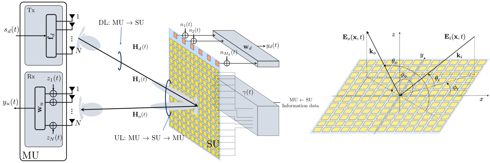
Let us consider the reference scenario depicted in Fig. 3, where a generic MU establishes a full-duplex link with a SU. To simplify, the MU is equipped with two uncoupled antenna arrays of meta-atoms each, to enable full-duplex capabilities at MU. The SU is equipped with a planar STMM of meta-atoms (along and respectively), and an Rx antenna array of meta-atoms. We assume that the STMM and the Rx array are co-located at the SU. The assumption concerning the SU is meant to conceptually separate for simplicity the device that receives MU SU data from the MU SU data stream via retro-reflection. Note that, it is possible to make a single device capable of both receiving and transmitting at the same time, for example, by connecting some meta-atoms of the metasurface to one (or more) RF chain [29]. In this case, the analytical derivations would be slightly different, but the results are equivalent to those investigated herein.
III-A Signal model
The time-continuous signal from the MU can be generally expressed as:
| (9) |
where is the spatial precoding vector and is the MU SU time-continuous base-band information signal with bandwidth , centered around the carrier frequency . The MU SU signal propagates over a high-frequency channel [30], yielding a received signal at the SU:
| (10) |
where represents the MU SU path loss in power, * is the matrix convolution, is the SU spatial combiner, is the MU SU MIMO channel matrix, such that while is the additive noise, spatially and temporally uncorrelated.
The Rx signal model at the MU can be evaluated by considering the propagation towards the STMM and its retro-reflection to the MU. The MU SU signal at the STMM is
| (11) |
where is the forward MIMO channel between the MU and the STMM. The signal undergoes the STMM phase reflection and then the convolution with the backward (MU SU) MIMO channel , obtaining:
| (12) |
where is the UL path loss in power, is the uplink combiner at the MU, is the additive noise at the MU array and denotes the time-varying STMM phase pattern matrix
| (13) |
where the time-varying phase matrix is obtained by discretizing the reflection coefficient in (5) over the spatial dimension, i.e., the STMM is modeled as a modulated reflectarray with regularly spaced meta-atoms. In particular, the relative position of the -th meta-atom of the STMM w.r.t. to the phase center is , for , , being and being the meta-atoms spacing along the and axes, respectively. Notice that, although is a time-varying function, the relation with is multiplicative because the time-varying signal injected by the STMM is a reflection coefficient.
Remark 1: Precoding and combining vectors, i.e., and (, ), are herein based on the knowledge of channels and , at both MU and SU side. Notice that channel estimation at the SU can be obtained through conventional approaches and shared with the MU through feedback [31].
Remark 2: Decoding of the MU SU information signal in is possible thanks to the knowledge of the MU SU one , that shall be removed by the MU to obtain (not analyzed here).
III-B Channel Model
The cluster-based multipath channel model is widely used in the design of mmWave and sub-THz wireless communication systems because it effectively captures the unique propagation characteristics of these frequencies [32]. This model is used here since this paper is framed for these frequencies. The -th entry of any of the channel impulse responses in (10)-(12) can be written as
| (14) |
where (i) is the number of paths, (ii) is the scattering amplitude of -th path, such that , (iii) is the propagation delay of the -th path from the phase center of the Tx to the phase center of the Rx, (iv) and are the residual propagation delays due to the position of the -th Tx meta-atom and the -th Rx meta-atom w.r.t. to their phase centers. As common for communication systems operating through back-scattering, the two-way channel to/from the STMM is characterized by a single dominant path, as for radar systems [33]. However, the technical extent of this work is not limited by the latter assumption. Multiple bounces (i.e., multipath forward and backward channels) can be considered, but (i) their path loss is usually higher (or much higher) w.r.t. the direct MU SU path, except for pure reflections in the environment (e.g., walls) and (ii) both MU and SU are spatially selective, thus multipath components outside the main radiation lobe of the MU (or SU) would be strongly attenuated. The combination of spatial selectivity and increased path-loss allows us to reasonably assume for both forward and backward channels. Considering a single path yields a common propagation delay between MU and SU and residual delays at the STMM that depend on the incidence and reflection angles , (coincident for full-duplex settings such as the one depicted in Fig. 3). The expression of the residual delay at the STMM is shown in Section IV-A. The inter-meta-atom spacing of Tx and Rx arrays (at both MU and SU) is , while at STMM is . The propagation path losses in power, and in (10)-(12) are modeled as [34]
| (15) |
where is the MU-SU distance. The model in (15) is obtained by assuming that the effective area of the MU/SU arrays is equal to the physical one, which is approximated as , and that the retro-reflected cross-section of the STMM is equal to the one of a perfect metallic plate with an area of as if it is oriented towards the MU [34].
Remark: The MU SU path loss is here assumed as only dependent on the wavelength of the incident signal . As detailed in Section IV, this is true for STMM phases considered as stochastic, whose average time derivative is zero, i.e., , as common for information-bearing signals. Differently, for , (e.g., a simple frequency shifting), the denominator of would be , with derived from (8).
IV Temporal Modulation


This section defines the principles of temporal modulation at the STMM and its peculiarities. For the implementation of the STMM, we propose two potential architectures, as depicted in Fig. 4. The first architecture, A, models each meta-atom with space-time tunability. Alternatively, architecture B models each meta-atom with spatial tunability and a single tunable component for temporal control shared with all meta-atoms. The difference between A and B is mainly the reduced cost/complexity of the second, which comes at the price of a slightly reduced performance, as will be discussed in the following. This dissimilarity arises from the fact that temporal control requires fast-varying varactors to support very high data rates in the MU SU link, whereas spatial control can be achieved using cost-effective pin diodes. This discrepancy in component selection is attributed to the distinct operational demands of each control mechanism. To ease the derivation while maintaining the generality, we consider the MU to use precoding and combining vectors perfectly aligned with the SU. Thus, we have that and are given, e.g., estimated by conventional approaches [31].
IV-A Principles of Temporal Modulation
Let us consider the phase (13) applied at the STMM meta-atoms (architecture B) as the superposition of a spatial and a temporal component, such that at the -th meta-atom is
| (16) |
for , , where is the space component of the phase used to design a complete retro-reflection of the impinging signal and is an information-bearing phase signal applied at each STMM meta-atom, and common to all. Model (16), adopted in the current literature [20, 35] can also be considered valid for architecture A when only one data stream is generated at the SU, as considered in this paper.
| (17) |
where accounts for geometrical energy losses, while
| (18) |
is the residual propagation delay for the -th STMM meta-atom, located in (local STMM coordinates), and
| (19) |
are the propagation delays of the wavefront across two adjacent STMM meta-atoms displaced by along and . In (17), the first term is the complete expression of the Rx signal for MU SU and MU SU signals. Approximation implies that there are no spatially wideband effects at the STMM due to the MU SU signal, namely , where is the maximum delay across the STMM meta-atoms. This is equivalent to asserting that:
| (20) |
where is the symbol period of the MU SU information signal . In this setting, unwanted beam squinting from spatially wideband effects due to can be avoided (see [36] for details). With approximation , the MU SU signal undergoes a multiplicative channel that encodes the MU SU phase signal , whose structure is discussed in Section IV-B. Similarly, approximation subtends that the MU SU phase-only signal does not suffer the relative propagation delay across the STMM, thus , or, equivalently
| (21) |
where is the symbol period of the MU SU phase signal . Approximation in (17) has the further implication that the spatial phase component is not affected by the temporal one , i.e., they can be separated and, consequently, the reflection gain is maximized by a phase-only pattern (not a function of time) across the STMM:
| (22) |
leading to the multiplicative model [20]
| (23) |
where denotes the MU SU signal injected by the STMM modulating the MU signal .
However, model (23) that is typically assumed in the existing literature on STMM is valid in restricted settings (e.g., and , as in [20]). Generally, neither approximation nor approximation hold for large-bandwidth systems and/or comparatively large STMM. Noteworthy, while the beam squinting due to cannot be compensated (except by reducing the MU SU bandwidth ), the coupling between spatial and temporal phase patterns for is peculiar to the STMM when involving wireless systems. The detrimental effect analyzed herein is the coupling between the spatial and temporal phases. Therefore, solutions to space-time phase coupling are detailed in Section IV-B and proposing countermeasure for wideband MU SU system is in Section IV-C.
IV-B Space-Time Phase Coupling
The space-time phase coupling can be readily explained considering Fig. 4. A plane wave impinging on the -th meta-atom of the STMM with angle , as depicted in Fig. 4, will be retro-reflected with the following phase:
| (24) |
thus the phase experiences a meta-atom-specific time delay that depends on the incidence angles , which induces a spurious, and undesired, spatial phase gradient. This phenomenon leads to an unwanted decrease in the reflection gain. In other words, assuming the conventional spatial phase gradient detailed in (22), we have that the following theorem holds:
Theorem 1.
Proof.
The proof can be readily carried out by inspection of the structure of , which yields
| (26) |
To have equality in (26), the arguments of the complex exponential shall neither be a function of nor of (spatial and temporal phase decoupling). Therefore, the sufficient conditions are (straightforward condition) or (). ∎
Theorem 1 implies that any phase-encoded modulation signal leads to a strict inequality for (26), except for very low MU SU signal bandwidth, fulfilling (21), or the case in which the impinging wave is perfectly orthogonal to the STMM plane, i.e., . To evaluate the space-time phase coupling effect, let us consider a generic non-linear , infinitely differentiable for . We can use the Taylor expansion around , truncated at the -th term
| (27) |
where denotes the -th time derivative of evaluated in . Considering only the first order () derivative only, namely
| (28) |
the second term is a linear phase shift with the meta-atom index that results in the so-called beam squinting, i.e., the angular shift of the reflected beam w.r.t. to the desired direction . This effect causes a reduction of the reflection gain that can be analytically evaluated from the STMM’s array factor that adds up to a possible beam squinting due to a large bandwidth (herein not considered).
To quantify the beam squinting due to (28), let us consider a linear temporal phase signal (or piecewise linear, e.g., obtained with frequency shift keying (FSK) modulation) , where is the frequency shift determined by the temporal component of the phase as in (8). Let us express the frequency shift as , where is a coefficient that describes the frequency up- or down-conversion, or equivalently . By substituting the expression of in (26) and removing the expectation, we obtain
| (29) |
with the corresponding normalized reflection gain in (30).
| (30) |
Considering for instance a 1D case (i.e., either a 1D STMM or ), replacing in (18) with in (19) (), the normalized reflection gain simplifies as
| (31) |
This allows gaining insight into the effective reflection gain of the STMM. Fig. 5 depicts the impact of the space-time phase coupling on the normalized reflection gain, and for and , the system experiences a diminished reflection gain. For instance, at we observe a loss dB () and dB () for % (e.g., for a frequency shift of GHz around GHz). The loss w.r.t. the maximum reflection gain can be justified by the tilting of the direction of maximum reflection, which can be evaluated as
| (32) |
where is the angle of maximum reflection, different from the true one due to the space-time phase gradient coupling. The trend of with the frequency shift is shown in Fig. 6. The result in (32) is obtained by substituting (28) and (22) in (17). Note that for in (32) we have evanescent waves, as depicted in Fig.7.

Whenever the phase is periodic, or cyclo-stationary, the aforementioned approaches are specialized to the harmonics of the Fourier series decomposition of as experimentally observed in [17, 18]. To implement a wireless communication system using STMM technology, the spatial phase must be decoupled from the temporal one, such that the former can be used to retro-reflect the impinging signal toward the MU and the latter to convey information.
IV-C Space-Time Phase Decoupling
Decoupling the spatial phase from the temporal phase can be achieved differently depending on the specific STMM architecture.
IV-C1 Architecture A
Decoupling can be achieved by delaying the temporal phase of each meta-atom to compensate for the propagation delay caused by the wavefront. Specifically, the phase of the -th meta-atom must be set as:
| (33) |
To achieve perfect decoupling, assumed herein, the STMM meta-atoms must be accurately time-synchronized using the knowledge of the incident angles as input, e.g., after a proper estimation.
IV-C2 Architecture B
A straightforward yet effective countermeasure to space-time phase coupling is to pre-compensate the spatial phase by considering the induced effect of the temporal phase. In particular, the phase of the -th meta-atom is
| (34) |
where the spatial phase now incorporates the meta-atom-dependent delay . As demonstrated in Section VI, architecture B allows for a cost reduction (only a single tunable component is used to control the temporal phase) compared to architecture A, at the price of performance reduction for large bandwidth UL signals. The design of , the requirements, and the achievable performance of the proposed communication system are discussed in the following Section V.
V UL Signal Design
The MU SU signal can be designed following conventional methods (e.g., linear modulation or orthogonal frequency division multiplexing). In this section, we propose the criteria to design the phase shape for controlled retro-reflection by the STMM.
V-A Continuous Phase Modulation
Let us consider that is a CPM signal for MU SU:
| (35) |
where is the modulation index, , , is the -th -ary information symbol, is the MU SU symbol duration, and is the phase pulse with the following properties
| (36) |
where represents the modulation memory. The phase pulse is usually defined as
| (37) |
with being the pulse shaping filter (PSF). The reason behind choosing CPM is that it represents the most general phase modulation for . Indeed, depending on the parameters set , and , the CPM can degenerate in the other phase modulations, such as phase shift keying (PSK), frequency shift keying (FSK), minimum shift keying (MSK), and Gaussian MSK (GMSK) [37]. The same reference can be used as an introduction to CPM.
V-B Bandwidth Occupancy
The bandwidth occupied by the MU SU received signal in (10), assuming a frequency-flat channel, is the bandwidth of the transmitted signal , i.e., the support of the power spectral density (PSD) , where denotes the Fourier Transform operator. Under the same channel assumption, the bandwidth occupied by the MU SU signal in (12), is the support of its PSD, defined as
| (38) |
and thus, according to the properties of the convolution, the total bandwidth of the system is
| (39) |
with being the support of . Notice that the resulting spectrum is centered around the carrier frequency . This follows from the fact that the information-bearing phase signal has the time-derivative
| (40) |
that is zero on the ensemble average, i.e., , thus the average net frequency shift is zero. For a generic CPM signal, the occupied bandwidth is infinite, but, the of the signal energy is within [38]
| (41) |
where is the time-bandwidth product of the specific CPM implementation. In (41), the term depends on the PSF used, e.g., for rectangular and for raised cosine. The bandwidth occupation is inversely proportional to the CPM memory . For , (rectangular PSF), the bandwidth is .
It is worth underlining that the proposed communication system is full-duplex, as MU SU and MU SU communications simultaneously occur on the same spectrum portion . However, the spectral efficiency is equivalent to an FDD system, with for MU SU and for MU SU, as detailed in the following.
V-C Spectral Efficiency
The performance of the proposed system can be assessed in terms of spectral efficiency (SE), considering both MU SU and MU SU links. In particular, the SE upper bound given by Shannon’s unconstrained SE is:
| (42) |
where the first term () is the SE of the MU SU and the second () is the SE of the MU SU. In (42), is the fractional bandwidth occupied by the MU SU, and the MU SU counterpart, while and are the MU SU and MU SU signal-to-noise ratios (SNRs) at the decision variable.
The MU SU SNR is
| (43) |
where the equality holds when perfect CSI is available and optimal precoding/combing is employed, both providing the maximum MIMO gain, i.e., .
The MU SU Rx signal undergoes a matched filtering over with the Tx signal , which is clearly known at MU. Assuming the delay is known, the SNR can be analytically evaluated as in Appendix A, depending on whether the STMM exhibits a wideband behavior w.r.t. or not. A suitable upper bound on the SNR is obtained by assuming that the wideband regime involves the same UL symbol, i.e., , yielding
| (44) |
where is the loss due to the space-time phase coupling, defined in (30), and is the processing gain of the matched filter. The latter is motivated by the fact that, while the MU SU noise occupies the whole bandwidth , the signal only occupies a fraction of it . Thus, the matched filter makes the MU SU SNR inversely proportional to the fractional bandwidth occupation, . The equality in (44) holds under the following conditions: (i) perfect CSI available at both MU and SU, (ii) known delay at the MU, and (iii) constant phase .
The MU SU and MU SU capacity in (42) has a global optimum with respect to the unconstrained UL bandwidth allocation . From the derivative of w.r.t.
| (45) |
whose root provides the optimal duplexing allocation. In (45), we denote with the MU SU SNR terms that do not depend on the allocation . The total capacity is analyzed in Section VI.
VI Numerical Results
This section presents numerical and analytical results for the proposed STMM-based wireless communication system, aimed at gaining insight into upper achievable performance, operating conditions, and possible limitations. In all the following, the frequency of operation is GHz. We consider a CPM modulation with a rectangular PSF, , and -ary, where . This coincides with CP-FSK for (herein considered) and with MSK for . The trends and considerations are the same for a generic CPM or any phase/frequency modulation, but the absolute values must be derived case by case.
VI-A Impact of system parameters
The first set of results, summarized in Fig. 8, shows the achievable SE (both MU SU and MU SU) varying system parameters, in the utter performance assumption of , namely with (44), which is commonly assumed in the state of the art on STMM [20]. These results can be attained for (i) architecture A with space-time decoupling (33), (ii) architecture B with space-time decoupling (34) and limited bandwidth , and (iii) normal incidence, i.e., deg. In all cases, we have , thus the same bandwidth for MU SU and MU SU. Fig. 8a shows the SE varying the MU SU equivalent single-input single-output (SISO) SNR, namely
| (46) |
as well as the number of MU antennas and STMM meta-atoms . The MU SU link length is fixed to m and the number of SU Rx meta-atoms . We notice the dramatic impact of the number of STMM meta-atoms that allows boosting the MU SU SE (up to be higher than the MU SU one for ). A similar effect, though to a lesser extent, is obtained by increasing . The trend of the SE varying the MU SU link length is instead shown in Fig. 8b. For fixed MU SU performance , the UL one rapidly decays with , still being higher than the former one for massive MU arrays and STMM (i.e., a comparatively high number of STMM meta-atoms). As can be expected, when is fixed, e.g., by technological limitations, the overall MU SU SE is mostly ruled by the number of STMM meta-atoms , as confirmed by Fig. 8c, where the SE is let vary as a function of the STMM size (side number of meta-atoms ), for m and m. The results in Fig. 8 show that with an appropriate design, the STMM can provide excellent MU SU performance even at relatively large distances, comparable with the cell radius in current mmWave 5G systems. Remarkably, most of the energy employed to achieve and is spent at the MU, while the SU does not need a power amplifier. However, wideband effects due to the MU SU signal practically limit the performance and, mostly, the MU SU bandwidth , as discussed in the following.
VI-B Impact of space-time phase coupling and decoupling
The wideband effects on the STMM operation are investigated in Fig. 9, reporting the MU SU SE varying , i.e., the equivalent linear frequency shift due to the modulating signal . We assume (i) , such that to ignore any wideband effect due to the MU SU signal , that is the approximation (a) in (17) and (ii) perfect channel state information (CSI) is available at the SU, namely the incidence/reflection angles are perfectly known. The distance is m and . The aim of these results is to quantitatively examine the impact of the space-time phase coupling at the STMM, while the impact on an imperfect CSI is discussed in the next set of results. The analysis in Section IV-B has shown that the space-time coupling is not influenced by transmitted power or distance, but rather by MU SU bandwidth , angle of incidence/reflection , and the size of the STMM . Fig. 9 considers both architectures A and B, with ideal compensations (33)-(34), respectively, and two incidence angles, deg ( deg for simplicity). The non-compensation case is shown as a benchmark. architecture A has the best performance, independent of , thanks to the possibility of compensating for the two-way delay at each meta-atom of the STMM. Considering architecture B, instead, where only one time-varying component is present (and common to all the STMM meta-atoms), the UL SE progressively degrades for increasing grazing incidence angles ( deg) and STMM meta-atoms . In both Fig. 9a and 9b, we can distinguish three operation regions, outlined in Appendix A and corresponding to (i) , i.e., ideal narrowband STMM operation; (ii) , i.e., wideband STMM operation without ISI; (iii) , i.e., wideband STMM operation with ISI. The first operation region occurs for very low modulation bandwidths (e.g., for , deg and for , deg), limiting the effective MU SU throughput. The second operation region happens for larger modulation bandwidths, up to a cut-off frequency (e.g., for , deg and for , deg). In this regime, the STMM benefits from the space-time decoupling (34) to improve the SE up to bit/s/Hz (for in Fig. 9b). Above the cut-off limit , the STMM realized with architecture B does not work properly: the SNR after the matched filter is abated by the presence of the ISI from past modulation symbols in (see Appendix A). The performance rapidly drops to zero. It is worth remarking that past symbols represent ISI as far as the simple matched filter approach (before trellis decoding) is adopted. In principle, the Rx can be designed to account for the unwanted additional delay due to the STMM reflection, attaining a similar performance to architecture A; however, this would increase the complexity of the implementation and it is not considered here. Alternatively, a viable solution may be to consider an STMM that combines the advantages of architectures A and B, e.g., by allowing the delay tuning at different subsets of meta-atoms.


VI-C Impact of imperfect CSI
In practice, incidence/reflection angles are estimated at the SU Rx array, leading to unavoidable errors affecting both the spatial phase configuration of the STMM (imperfect pointing) as well as the space-time phase decoupling (imperfect compensation). The combination of the latter two effects has the consequence of diminishing the amount of Rx signal energy at the MU side, decreasing the SE w.r.t. the ideal case (see Appendix B for the analytical derivations). Fig. 10 shows the MUSU SE varying the equivalent SISO SNR (46), with and without space-time decoupling (as in [20]) and in presence of errors on the estimation of the elevation angle , whose variance is quantified herein with the Cramér-Rao lower bound (CRLB) [39] (Appendix B). We consider the very same simulation parameters used for Fig. 8a, namely Tx antennas at the MU, Rx antennas at the SU, deg, deg (known), (Fig. 10a), (Fig. 10b). With the current settings, the standard deviation of the error on ranges from deg at dB to deg at dB. As a further benchmark, we show the constrained SE of a backscatter communication system where the STMM is OOK-modulated, with no space-time phase decoupling and imperfect CSI as well [22]. In the low SNR region, the error on the estimation of (ruled by ) jeopardizes any space-time phase decoupling effort. Namely, the imperfect pointing caused by a wrong setting of the spatial STMM phase (red curves) is much larger than the effect of the space-time phase coupling counterpart (yellow curves). Notice that yellow curves represent the performance of state-of-the-art works on STMM-based wireless systems [20], where is assumed to be perfectly known but the space-time coupling is not compensated. However, as grows large, the performance trend swaps: the effect of the imperfect CSI vanishes (red curves attain the blue ones asymptotically) and only an uncompensated space-time phase coupling affects the performance. Of course, as the spatial selectivity of the STMM increases (), the impact of imperfect CSI and coupling gets worse. Interestingly, we observe a threshold SNR value (depending on the size of of the STMM ) that determines two operating regions: for , the SE is dominated by the effect of CSI errors (requiring proper countermeasures, e.g., increasing the Rx array size ), while for , the performance is dominated by the space-time phase coupling, confirming the outcomes of Fig. 9 and requiring the suitable compensation proposed in this work. In any case, the proposed STMM-based wireless communication system outperforms the OOK-modulated one, which only employs a two-level amplitude modulation (yielding a -3 dB matched filter gain at the MU) and does not operate any compensation for the space-time phase coupling.
VI-D Impact of the bandwidth ratio
Concerning the optimal choice of , namely the bandwidth splitting between MU SU and MU SU, it depends on the size of the STMM and the distance between the MU and SU. Fig. 11 shows the MU SU, MU SU, and total SE , and respectively, varying for m, , and assuming ideal narrowband STMM behavior (upper-performance limit). The total SE shows a peak, as predicted by (45), that depends on the number of STMM meta-atoms . This result can have two readings: one can maximize the spectral efficiency over the entire bandwidth , and thus the fraction allocated depends on the specific setup, or one can allocate the fraction based on the MU and SU requirements, but the spectral efficiency over the entire band may not be optimal. In other words, the method used to allocate the fraction of the band can be based on either maximizing overall spectral efficiency or on specific MU and SU requirements. While maximizing overall spectral efficiency is desirable in some cases, it may not be the best approach if the MU and SU requirements must be met. In such cases, one may have to compromise on the overall spectral efficiency to meet the requirements of the MU and SU.
VII Conclusions and Open Challenges
This paper proposes a mathematical model for the design of STMMs in wireless communication systems, where the spatial component of the modulation controls the direction in which the signal is reflected, and the temporal component conveys information in the designated direction. The model examines two potential implementations, Architectures A and B, with Architecture A having greater design flexibility than Architecture B, which is more cost-effective. The model describes the unique features of the STMMs, including the space-time phase coupling and how it affects system performance. Analytical descriptions of these effects are provided, along with suggested countermeasures. Additionally, the proposed model addresses the design criteria and challenges of STMM-based wireless communications, specifically in the context of a full-duplex system architecture, which is one of the promising solutions where STMMs can be beneficial. The full-duplex system architecture comprises a master unit (MU) that transmits a downlink MU SU signal and a slave unit (SU) that can receive, reflect, and modulate the MU SU using STMM technology. In order to transmit information in uplink MU SU, the SU modulates the temporal phase gradient applied to the metasurface meta-atoms. To validate the analytical findings, numerical results are presented, demonstrating the efficacy of the proposed model, even in the presence of imperfect CSI acquisition. Nonetheless, the proposed mathematical model only serves as an initial step for designing and analyzing STMM-based wireless communication systems. Further research is imperative to fully explore the capabilities and limitations of STMM technology. This should include investigations into multi-user scenarios, the impact of mobility on system performance, and experimental validations to bridge the gap between theory and practical implementation. Addressing these challenges will pave the way for harnessing the full potential of STMMs in future wireless communication applications.
Appendix A
The Rx signal at the MU side undergoes matched filtering and phase estimation, before being fed to the sequence detector, e.g., Viterbi. We derive the SNR after the matched filter at the MU in the assumption that the Rx signal is the one expressed by (17), approximation . The estimated phase at the -th MU SU symbol is provided by
| (47) |
The SNR is obtained from with a double expectation over the Tx signal and the modulating phase . The power of the useful signal part is in (48),
| (48) |
where we made use of the Schwartz inequality and assume, for simplicity of exposition, that the MU SU signal has a constant power within the integration interval . According to the size of the STMM compared to the MU SU bandwidth (related to the symbol time through (41)), we can distinguish three cases, as detailed in the following.
A-1
In this case, the STMM exhibits a narrowband behavior w.r.t. to the MU SU signal, namely the variation of across the STMM can be neglected. Therefore, we have
| (49) |
and the reflection gain is maximized under the assumption of the perfect knowledge of the channel (i.e., perfect spatial phase configuration in (41)). The power of the noise after the matched filter is
| (50) |
(including the beamforming gain at the MU), thus the SNR is upper-bounded by
| (51) |
from which follows (44) by expanding .
A-2
In this case, the STMM exhibits a wideband behavior w.r.t. to the MU SU signal, namely the variation of across the STMM cannot be ignored in (48), but it is less then the symbol duration. Now, we have
| (52) |
it yields the case explored in Section IV with the beam squinting effect. The SNR upper bound is
| (53) |
The previous expression tends to be the narrowband one when applying compensation techniques in Section IV-C.
A-3
In this case, the STMM exhibits a wideband behavior w.r.t. to the MU SU signal and the variation of across the STMM exceeds the symbol duration. This means that the MU receives a signal with multiple superposed symbols, and the STMM meta-atoms can be clustered according to the specific MU SU symbol they are reflecting at a given instant of time. Considering for simplicity a linear STMM, we have spanned symbols, where is the propagation delay across two adjacent meta-atoms, . Considering a 2D STMM again, we can define the following set of STMM meta-atoms:
| (54) |
for , , where the first one indicates the symbol of interest and the second all the remaining ones. Notice that estimating the phase with the simple matched filter in (47) implies that the symbols other than the -th of interest act as inter-symbol interference (ISI). Therefore, we have the relation in (55)
| (55) |
and thus the useful signal power is
| (56) |
while the ISI power comes from the integration across different symbols, with detrimental effects on system performance. The SNR turns into SINR as
| (57) |
Appendix B
This Appendix derives the model for the characterization of the system performance in case of imperfect CSI, i.e., when the incident elevation angle is estimated with unavoidable error at the SU side, . Extension to the case in which is subject to estimation errors is possible but covered here, thus we consider (and ) to ease the derivations. We herein consider, for simplicity, that (i) the estimated angle is Gaussian-distributed, i.e., and (ii) the estimation attains the CRLB, hence the variance of the error is [39]:
| (58) |
Let us consider the Rx signal (17) , where we apply the following space-time phase at the STMM (with decoupling as for (33))
| (59) |
where
| (60) |
(the approximation is for small ). We obtain from (17):
| (61) |
where equality holds by considering a linearly time-varying phase (or piece-wise linear) and approximation is for small . Notice that (61) resembles the ideal multiplicative model (23), except for the residual summation, representing the loss due to imperfect estimation of . We can distinguish between two effects: the imperfect pointing, due to errors in the spatial phase configuration, and the imperfect decoupling, due to errors in the compensation of the residual delay at the STMM. The ensemble average of the energy loss at the MU side due to imperfect CSI can be evaluated from (61) as follows:
| (62) |
where the expectation is carried out over the distribution of , and the overall effects are shown in Section VI-C.
References
- [1] W. Saad, M. Bennis, and M. Chen, “A vision of 6G wireless systems: Applications, trends, technologies, and open research problems,” IEEE Network, vol. 34, no. 3, pp. 134–142, 2020.
- [2] M. Mizmizi, M. Brambilla, D. Tagliaferri, C. Mazzucco, M. Debbah, T. Mach, R. Simeone, S. Mandelli, V. Frascolla, R. Lombardi et al., “6g v2x technologies and orchestrated sensing for autonomous driving,” arXiv preprint arXiv:2106.16146, 2021.
- [3] M. Di Renzo, A. Zappone, M. Debbah, M.-S. Alouini, C. Yuen, J. De Rosny, and S. Tretyakov, “Smart radio environments empowered by reconfigurable intelligent surfaces: How it works, state of research, and the road ahead,” IEEE Journal on Selected Areas in Communications, vol. 38, no. 11, pp. 2450–2525, 2020.
- [4] A. M. Elbir, K. V. Mishra, M. R. B. Shankar, and S. Chatzinotas, “The rise of intelligent reflecting surfaces in integrated sensing and communications paradigms,” IEEE Network, pp. 1–8, 2022.
- [5] Y. Zhang, J. Zhang, M. Di Renzo, H. Xiao, and B. Ai, “Performance analysis of ris-aided systems with practical phase shift and amplitude response,” IEEE Transactions on Vehicular Technology, 2021.
- [6] L. Jiao, P. Wang, A. Alipour-Fanid, H. Zeng, and K. Zeng, “Enabling efficient blockage-aware handover in ris-assisted mmwave cellular networks,” IEEE Transactions on Wireless Communications, pp. 1–1, 2021.
- [7] M. Mizmizi, R. A. Ayoubi, D. Tagliaferri, K. Dong, G. G. Gentili, and U. Spagnolini, “Conformal metasurfaces: a novel solution for vehicular communications,” IEEE Transactions on Wireless Communications, pp. 1–1, 2022.
- [8] D. Tagliaferri, M. Mizmizi, R. A. Ayoubi, G. G. Gentili, and U. Spagnolini, “Conformal intelligent reflecting surfaces for 6g v2v communications,” in 2022 1st International Conference on 6G Networking (6GNet), 2022, pp. 1–8.
- [9] M. Mizmizi, D. Tagliaferri, M. Khosronejad, L. Resteghini, G. G. Gentili, L. Draghi, and U. Spagnolini, “Conformal metasurfaces for recovering dynamic blockage in vehicular systems,” in GLOBECOM 2022 - 2022 IEEE Global Communications Conference, 2022, pp. 6025–6030.
- [10] Y. U. Ozcan, O. Ozdemir, and G. K. Kurt, “Reconfigurable intelligent surfaces for the connectivity of autonomous vehicles,” IEEE Transactions on Vehicular Technology, vol. 70, no. 3, pp. 2508–2513, 2021.
- [11] S. Buzzi, E. Grossi, M. Lops, and L. Venturino, “Foundations of mimo radar detection aided by reconfigurable intelligent surfaces,” IEEE Transactions on Signal Processing, vol. 70, pp. 1749–1763, 2022.
- [12] N. Yu, P. Genevet, M. A. Kats, F. Aieta, J.-P. Tetienne, F. Capasso, and Z. Gaburro, “Light propagation with phase discontinuities: Generalized laws of reflection and refraction,” Science, vol. 334, no. 6054, pp. 333–337, 2011. [Online]. Available: https://www.science.org/doi/abs/10.1126/science.1210713
- [13] A. Shaltout, A. Kildishev, and V. Shalaev, “Time-varying metasurfaces and lorentz non-reciprocity,” Optical Materials Express, vol. 5, no. 11, pp. 2459–2467, 2015.
- [14] Y. Hadad, D. L. Sounas, and A. Alu, “Space-time gradient metasurfaces,” Physical Review B, vol. 92, no. 10, p. 100304, 2015.
- [15] S. Taravati and G. V. Eleftheriades, “Microwave space-time-modulated metasurfaces,” ACS Photonics, vol. 9, no. 2, pp. 305–318, 2022.
- [16] L. Zhang, X. Q. Chen, S. Liu, Q. Zhang, J. Zhao, J. Y. Dai, G. D. Bai, X. Wan, Q. Cheng, G. Castaldi, V. Galdi, and T. J. Cui, “Space-time-coding digital metasurfaces,” Nature Communications, vol. 9, no. 1, p. 4334, Oct 2018.
- [17] Zhang, Lei, Dai, Jun Yan, Moccia, Massimo, Castaldi, Giuseppe, Cui, Tie Jun, and Galdi, Vincenzo, “Recent advances and perspectives on space-time coding digital metasurfaces,” EPJ Appl. Metamat., vol. 7, p. 7, 2020. [Online]. Available: https://doi.org/10.1051/epjam/2020007
- [18] L. Zhang and T. Cui, “Space-time-coding digital metasurfaces: Principles and applications,” Research, vol. 2021, pp. 1–25, 05 2021.
- [19] G.-B. Wu, J. Dai, Q. Cheng, T. Cui, and C. Chan, “Sideband-free space–time-coding metasurface antennas,” Nature Electronics, vol. 5, no. 11, p. 808–819, Nov. 2022.
- [20] W. Tang, J. Y. Dai, M. Z. Chen, K.-K. Wong, X. Li, X. Zhao, S. Jin, Q. Cheng, and T. J. Cui, “Mimo transmission through reconfigurable intelligent surface: System design, analysis, and implementation,” IEEE Journal on Selected Areas in Communications, vol. 38, no. 11, pp. 2683–2699, 2020.
- [21] J. Y. Dai, W. Tang, L. X. Yang, X. Li, M. Z. Chen, J. C. Ke, Q. Cheng, S. Jin, and T. J. Cui, “Realization of multi-modulation schemes for wireless communication by time-domain digital coding metasurface,” IEEE Transactions on Antennas and Propagation, vol. 68, no. 3, pp. 1618–1627, 2020.
- [22] Y.-C. Liang, Q. Zhang, J. Wang, R. Long, H. Zhou, and G. Yang, “Backscatter communication assisted by reconfigurable intelligent surfaces,” Proceedings of the IEEE, vol. 110, no. 9, pp. 1339–1357, 2022.
- [23] G. Lin, A. Elzanaty, and M.-S. Alouini, “Lora backscatter communications: Temporal, spectral, and error performance analysis,” IEEE Internet of Things Journal, pp. 1–1, 2023.
- [24] A. H. Raghavendra, A. K. Kowshik, S. Gurugopinath, S. Muhaidat, and C. Tellambura, “Generalized space shift keying for ambient backscatter communication,” IEEE Transactions on Communications, vol. 70, no. 8, pp. 5018–5029, 2022.
- [25] S. Y. Park and D. In Kim, “Intelligent reflecting surface-aided phase-shift backscatter communication,” in 2020 14th International Conference on Ubiquitous Information Management and Communication (IMCOM), 2020, pp. 1–5.
- [26] S. Xu, Y. Du, J. Liu, and J. Li, “Intelligent reflecting surface based backscatter communication for data offloading,” IEEE Transactions on Communications, vol. 70, no. 6, pp. 4211–4221, 2022.
- [27] S. Lin, F. Chen, M. Wen, Y. Feng, and M. Di Renzo, “Reconfigurable intelligent surface-aided quadrature reflection modulation for simultaneous passive beamforming and information transfer,” IEEE Transactions on Wireless Communications, vol. 21, no. 3, pp. 1469–1481, 2022.
- [28] A. Sabharwal, P. Schniter, D. Guo, D. W. Bliss, S. Rangarajan, and R. Wichman, “In-band full-duplex wireless: Challenges and opportunities,” IEEE Journal on Selected Areas in Communications, vol. 32, no. 9, pp. 1637–1652, 2014.
- [29] R. Schroeder, J. He, and M. Juntti, “Passive ris vs. hybrid ris: A comparative study on channel estimation,” in 2021 IEEE 93rd Vehicular Technology Conference (VTC2021-Spring), 2021, pp. 1–7.
- [30] T. S. Rappaport, Y. Xing, O. Kanhere, S. Ju, A. Madanayake, S. Mandal, A. Alkhateeb, and G. C. Trichopoulos, “Wireless communications and applications above 100 ghz: Opportunities and challenges for 6g and beyond,” IEEE access, vol. 7, pp. 78 729–78 757, 2019.
- [31] M. Mizmizi, D. Tagliaferri, D. Badini, C. Mazzucco, and U. Spagnolini, “Channel estimation for 6g v2x hybrid systems using multi-vehicular learning,” IEEE Access, vol. 9, pp. 95 775–95 790, 2021.
- [32] A. Meijerink and A. F. Molisch, “On the physical interpretation of the saleh–valenzuela model and the definition of its power delay profiles,” IEEE Transactions on Antennas and Propagation, vol. 62, no. 9, pp. 4780–4793, 2014.
- [33] M. Manzoni, D. Tagliaferri, M. Rizzi, S. Tebaldini, A. V. Monti-Guarnieri, C. M. Prati, M. Nicoli, I. Russo, S. Duque, C. Mazzucco, and U. Spagnolini, “Motion estimation and compensation in automotive mimo sar,” 2022.
- [34] S. Ellingson, “Path loss in reconfigurable intelligent surface-enabled channels,” in 2021 IEEE 32nd Annual International Symposium on Personal, Indoor and Mobile Radio Communications (PIMRC), 2021, pp. 829–835.
- [35] X. Fang, M. Li, D. Ding, F. Bilotti, and R. Chen, “Design of in-phase and quadrature two paths space-time-modulated metasurfaces,” IEEE Transactions on Antennas and Propagation, vol. 70, no. 7, pp. 5563–5573, 2022.
- [36] K. Dovelos, M. Matthaiou, H. Q. Ngo, and B. Bellalta, “Channel estimation and hybrid combining for wideband terahertz massive mimo systems,” IEEE Journal on Selected Areas in Communications, vol. 39, no. 6, pp. 1604–1620, 2021.
- [37] J. B. Anderson, T. Aulin, and C.-E. Sundberg, Digital phase modulation. Springer Science & Business Media, 2013.
- [38] C.-H. Kuo and K. M. Chugg, “On the bandwidth efficiency of cpm signals,” in IEEE MILCOM 2004. Military Communications Conference, 2004., vol. 1. IEEE, 2004, pp. 218–224.
- [39] A. Liu, Z. Huang, M. Li, Y. Wan, W. Li, T. X. Han, C. Liu, R. Du, D. K. P. Tan, J. Lu, Y. Shen, F. Colone, and K. Chetty, “A survey on fundamental limits of integrated sensing and communication,” IEEE Communications Surveys & Tutorials, vol. 24, no. 2, pp. 994–1034, 2022.