On Whitney extensions and orthonormal expansions

Throughout this paper $d\geq 2$, $n,m\geq 1$ and $|.|$ denotes the Euclidean norm on $\mathbb{R}^{n}$. Typically, most constants (most often denoted by $c,c_{1},..$) are always small enough and are independent of $d,n$ and possibly other quantities. The context will be clear. ^** * By small enough, we mean bounded by a controlled small constant. The analogy of large enough is clear.. If this is not explicitly stated, the context will be clear. The same letter may denote different constants and/or functions at any given time. The context will be clear. The classical Whitney extension problem asks the following: Let $\phi:E\to\mathbb{R}$ be a map defined on an arbitrary set $E\subset\mathbb{R}^{n}$. How can one decide whether $\phi$ extends to a map $\Phi:\mathbb{R}^{n}\to\mathbb{R}$ which agrees with $\phi$ on $E$ and is in $C^{m}(\mathbb{R}^{n})$, the space of functions from $\mathbb{R}^{n}$ to $\mathbb{R}$ whose derivatives of order $m$ are continuous and bounded.

In order to state one answer to this problem from the paper [32], we assume that $E$ is closed. We then ask for a theorem that says that it is possible to extend a given real valued function with domain $E$ in such a way as to have prescribed derivatives at the points of $E$. The set $E$ will in general, lack a differentiable structure and to this end we need a careful statement of Taylor’s theorem on $\mathbb{R}^{n}$ which provides an essential ingredient for the aforementioned theorem’s statement and proof. The theorem we state is that of Hassler Whitney [32] and is a partial converse to Taylor’s theorem.

A $n$-dimensional multi-index is an $n$-tuple of non-negative integers $\alpha=(\alpha_{1},....,\alpha_{n})$. We write $|\alpha|=\alpha_{1}+...+\alpha_{n}$, $\alpha!=\alpha_{1}!...\alpha_{n}!.$ For $x\in\mathbb{R}^{n}$, we write $x^{\alpha}=x_{1}^{\alpha_{1}}...x_{n}^{\alpha_{n}}$. Given a function $f:\mathbb{R}^{n}\to\mathbb{R}$ in $C^{m}(\mathbb{R}^{n})$, we set

when well defined.

We have Taylor’s theorem:  Let $f:\mathbb{R}^{n}\to\mathbb{R}$ in $C^{m}(\mathbb{R}^{n})$ at a point $a\in\mathbb{R}^{n}$. Then there exist functions $h_{\alpha}:\mathbb{R}^{n}\to\mathbb{R}$ with multi index $\alpha$ such that for $x\in\mathbb{R}^{n}$,

and $\lim_{x\to a}h_{\alpha}(x)=0.$

Differentiating and replacing $h_{\alpha}$ as needed (still denoted by $h_{\alpha}$), we obtain with $f_{\alpha}:=D^{\alpha}f$, for each multi index $\alpha$,

• (1)

  $f_{\alpha}(x)=\sum_{|\beta|\leq m-|\alpha|}\frac{f_{\alpha+\beta}(a)}{\beta!}(x-a)^{\alpha}+h_{\alpha}(x,a).$ with $h_{\alpha}=o(|x-a|)$ uniformly as $x\to a$.

We note that (1) may be regarded as purely a compatibility condition between the functions $f_{\alpha}$ which must be satisfied in order for these functions to be the coefficients of the Taylor series of the function $f$. This important observation allows us to deal with the problem of the closed set $E$, in general lacking a differentiable structure in the following Whitney theorem of Hassler Whitney [32] (below) which follows in part from it.

Let $\phi_{\alpha}:E\to\mathbb{R}$ be a collection of functions defined on a closed set $E\subset\mathbb{R}^{d}$ with all multi-indices $|\alpha|\leq m$ satisfying the compatibility condition (1) for all $x,a\in\mathbb{R}^{d}$. Then there exists a function $\Phi:\mathbb{R}^{d}\to\mathbb{R}$ in $C^{m}(\mathbb{R}^{d})$ such that the following hold:

• •

  $\Phi=\phi_{0}$.

• •

  $D^{\alpha}\Phi=\phi_{\alpha}$.

• •

  $\Phi$ is real-analytic in $\mathbb{R}^{d}\setminus E$.

Fourier series versus Taylor series

A holomorphic function in an anulus containing the unit circle has a Laurent series about zero which generalizes the Taylor series of a holomorphic function in a neighborhood of zero. When restricted to the unit circle, this Laurent series gives a Fourier series of the corresponding periodic function. This explains the connection between the Cauchy integral formula and the integral defining the coefficients of a Fourier series. The connection between the two provided by the Cauchy integral formula is therefore quite remarkable; one takes an integral of $f$ over the unit circle and it tells you information about the behavior of $f$ at the origin. But this is more a magic property of holomorphic functions than anything else. A variant of this argument would be the following: Assume that the Taylor expansion of a real valued function $f$: $f(x)=\sum_{k=0}^{\infty}a_{k}x^{k}$ is convergent for some $|x|>1$. Then $f$ can be extended in a natural way into the complex plane by writing $f(z)=\sum_{k=0}^{\infty}a_{k}z^{k}$ with $|z|\leq 1$. Restricting to the unit circle $|z|=1$, define $F(\phi):=f(e^{i\phi})$, that is, consider $f$ as a function of the polar angle $\phi$. $F$ has period $2\pi$ and its Fourier expansion is nothing else but $F(\phi)=\sum_{k=0}^{\infty}a_{k}e^{ik\phi}$ where the $a_{k}$ are the Taylor coefficients of the real valued map $x\longmapsto f(x)$

Our ultimate goal from this paper is to begin an exploration of relations between Witney extensions and orthonormal expansions in line with the above discussion and the interesting paper [13]. To this end, moving forward we will survey our work in [12, 2] and then state an interesting result of [13] (See Section 5) and raise some pertinent open questions related to these ideas.

We begin with:

In this section, we provide a small taiste of some of the work in [2] and refer the reader to the monograph [2] for the full adventure!

• •

  A map $A:\mathbb{R}^{d}\to\mathbb{R}^{d}$ is an improper Euclidean motion (rigid motion, distance preserving transformation) if there exist $M\in O(d)$ and a translation $x_{0}\in\mathbb{R}^{d}$ so that for every $x\in\mathbb{R}^{d}$, $A(x)=Mx+x_{0}$.

• •

  If $M\in SO(d)$, then $A$ is a proper (orientation preserving) Euclidean motion. Here, $O(d)$ and $SO(d)$ are respectively the orthogonal and special orthogonal groups. A Euclidean motion can either be proper or improper.

• •

  A map $f:\mathbb{R}^{d}\to\mathbb{R}^{d}$, will be called a $c$-distortion if there exists $c>0$ small enough depending on $d$ so that $(1-c)|x-y|\leq|f(x)-f(y)|\leq|x-y|(1+c)$ for every $x,y\in\mathbb{R}^{d}$. Note that $f$ is non-rigid.

The problems we are concerned with are:

• (1)

  Let $\phi:E\to\mathbb{R}^{d}$ be a smooth near distortion ^†† † When we use the term ”near distortion”, we mean $c$-distortion for small enough $c$. on a finite set $E\subset\mathbb{R}^{d}$ with certain geometry. How to decide whether $\phi$ extends to a smooth, one to one and onto near distortion $\Phi:\mathbb{R}^{d}\to\mathbb{R}^{d}$ which agrees with $\phi$ on $E$ and with Euclidean motions in $\mathbb{R}^{d}$.

• (2)

  Let $U\subset R^{n}$ be open and let $E\subset U$ be a compact set with certain geometry. Let $\phi:U\to\mathbb{R}^{n}$ be a smooth near isometry. How to decide if there exists a smooth one-to-one and onto near isometry $\Phi:\mathbb{R}^{n}\to\mathbb{R}^{n}$ which agrees with $\phi$ on $E$ and agrees with Euclidean motions on $\mathbb{R}^{n}$.

In [2], we study (1-2) in detail. This is a fascinating problem with connections to harmonic analysis, best approximation in algebraic varieties, algebraic geometry in particular, tensor analysis, alignment, clustering, the Procrustes alignment data problem, the manifold data learning problem and BMO (the space of maps of bounded mean variation). See also [1, 12, 16, 17, 18, 19, 20].

Problem (1) below is an example of (1) above:

In the case of isometric extension, Theorem 2 is less subtle. It is well known, see for example [31] that following holds..

Let $\left\{y_{1},...,y_{k}\right\}$ and $\left\{z_{1},...,z_{k}\right\}$ be two collections of $k\geq 1$ distinct points in $\mathbb{R}^{d}$. Suppose

Then, there exists a Euclidean motion, $A:\mathbb{R}^{d}\to\mathbb{R}^{d}$ with

Problem 1 and Problem 2 are a new way to view interpolation and non-rigid alignment of data. See [2] for the full details.

We now begin to look at Problem 1 and Problem 2. We will translate "smooth" into the idea of a $c$-distorted diffeomorphism.

Given $c$ small enough, a diffeomorphism $f:\mathbb{R}^{d}\to\mathbb{R}^{d}$ is a $c$-distorted diffeomorphism if $f$ is a $c$ distortion. ^¶¶ ¶ A diffeomorphism $f:\mathbb{R}^{d}\to\mathbb{R}^{d}$ is a differentiable one-to-one and onto function with a differentiable inverse.

We are now going to provide two examples of $c$-distorted diffeomorphisms.

Here are two examples: Take a function $f:\mathbb{R}^{2}\to\mathbb{R}$ and suppose (A) holds. Then

Take a function $f:\mathbb{R}^{3}\to\mathbb{R}$ and suppose (A) holds. Then

Here we illustrate the concept of a Slow twist on $\mathbb{R}^{2}$. Given a $\varepsilon>0$ and a function $f:\mathbb{R}^{2}\to\mathbb{R}$ so that (A) holds with the function $f$. Define the Slow twist matrix $T_{x}$ for any $x\in\mathbb{R}^{2}$ via

Then given any pure rotation $M\in\text{SO}(2)$, the following function $f_{St}(x):=M^{T}T_{x}Mx:\mathbb{R}^{2}\to\mathbb{R}^{2}$ is a Slow twist.

In $2$ dimensions, the rotation $M$ does not affect anything since rotations are commutative on $\mathbb{R}^{2}$. However, for higher dimensions this is not the case, and hence we leave them in the formulas, but for now we always fix $M$ to be the identity matrix. For a first set of illustrations, we will look only at one application of a Slow twist with $f$ being an exponential function with differing scaling parameter.

For large values of $c$ depending on $d$ the twist is near isometric, and even outside a small enough cube centered at the origin, the points are left essentially fixed. On the other hand, as $c$ tends to $0$, the twist becomes closer to a pure rotation near the origin. Nevertheless, at a far enough distance, the Slow twist $f_{ST}$ will leave the points essentially unchanged. Indeed, the next figures illustrate this:

Let us pause to consider what happens when the decay condition on the twist function $f$ (A) is not satisfied; in this case we will dub the twist function a Fast twist for reasons that will become apparent presently.

One can see that when $f$ is the identity function, the rate of twisting is proportional to the distance away from the origin, and hence there is no way that the twist function will leave points fixed outside of any ball centered at the origin. Likewise, one sees from that the Fast twist with function $f(x)=|x|^{2}$ rapidly degenerates points into a jumbled mess.

Here we illustrate what happens when one iteratively applies a Slow twist to a fixed initial point.

We see an illustration of the fact that the composition of Slow twists remains a Slow twist, but the distortion changes slightly; indeed, notice that as we take more iterations of the exponential Slow twist, we must go farther away from the origin before the new twist leaves the points unchanged.

We illustrate some simple examples of Slides on $\mathbb{R}^{2}$.

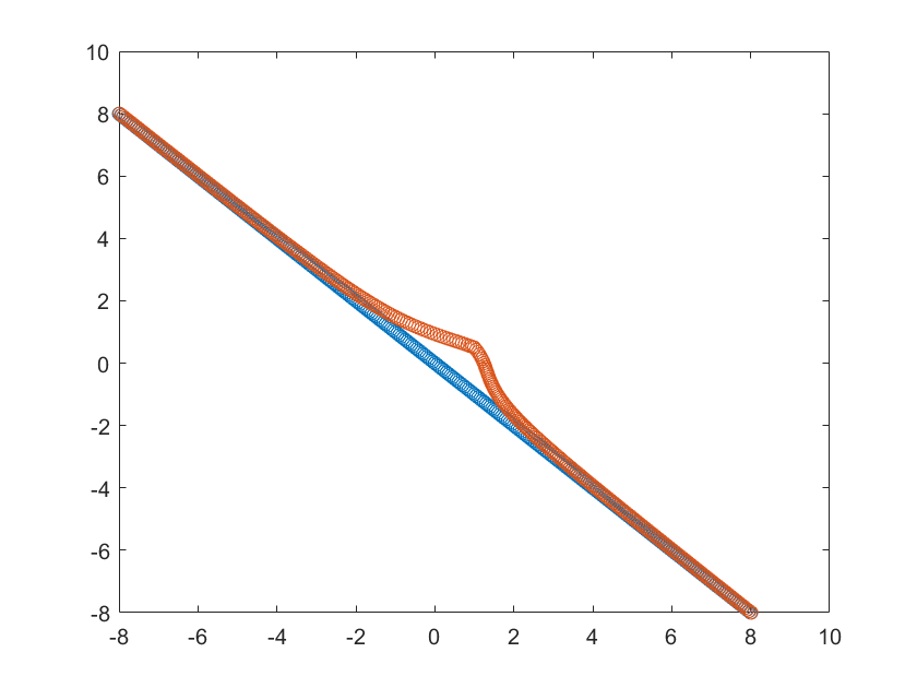
First consider equally spaced points on the line $y=-x$, and the Slide given by the function

This is illustrated in Figure 8.

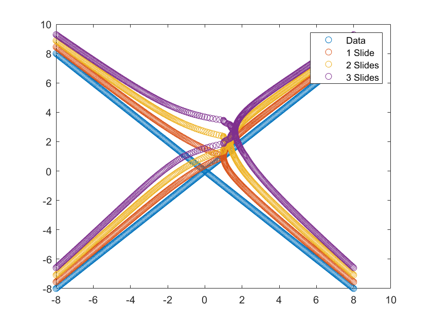
To give some more sophisticated examples, we consider first the Slide function

acting iteratively on uniform points along both the lines $y=x$ and $y=-x$.

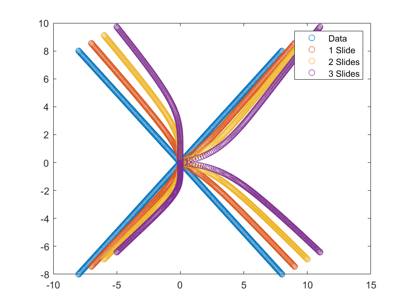
Similarly, the following figure shows the Slide function

acting iteratively on uniform points along the lines $y=x$ and $y=-x$.

To illustrate the effect of the distance of points from the origin, we illustrate here how Slides affect uniform points on circles of different radii.

We use again the asymmetric sliding function

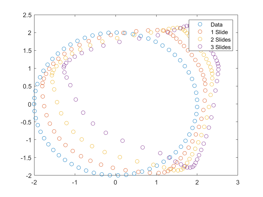
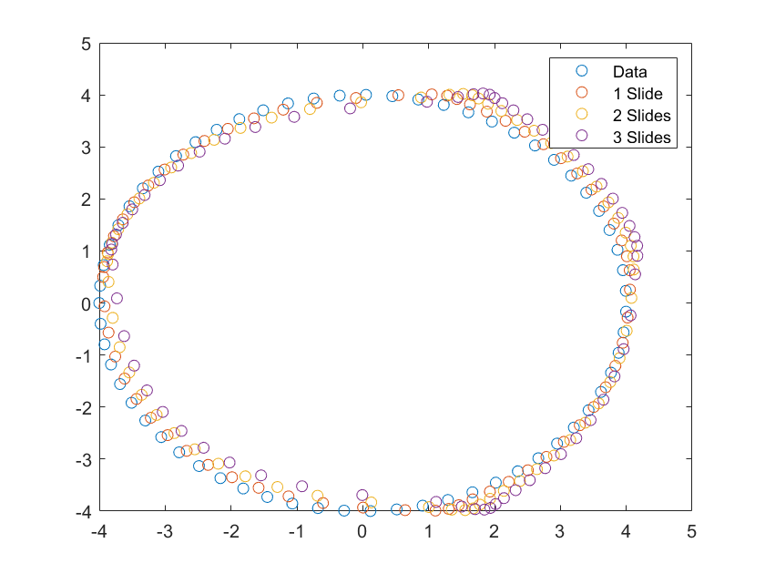
We see that the farther out the points are; i.e., the larger the radius of the initial circle, the less the effect of the Slide, which makes sense given the definition and the fact that the Slides must be $\varepsilon$–distortions of $\mathbb{R}^{2}$.

Here we illustrate some of the motions above in $\mathbb{R}^{3}$.

Here, we construct a generic rotation matrix in $SO(3)$ by specifying parameters $a,b,a_{1},d$ satisfying $a^{2}+b^{2}+a_{1}^{2}+d^{2}=1$, and the rotation matrix $M$ is defined by

As a reminder, our Slow twist on $\mathbb{R}^{3}$ is thus $M^{T}_{x}(Mx)$.

Here we generate 1000 random points on the unit sphere in $\mathbb{R}^{3}$ and allow them to move under a Slide formed by

From the definition of Slow twists and Slides, the following holds.

Moreover, we have:

We have then:

An important observation in Theorem 2.3 is that if $y_{i}=\phi(y_{i})$ for one $i=i_{0},\,1\leq i_{0}\leq k$, the extension $\Phi$ agrees with a Euclidean motion away from the set $E$. What this says is that if the function $\phi$ has a fixed point at one of the points of $E$, then the function $\Phi$ must be essentially rigid away from the set $E$. Note the unfortunate restriction of $k\leq d$ in Theorem 2.3(1). The good news is that the problem for this restriction occurs for only some degenerate cases and once removed, an explicit relation between the distortion constants $\varepsilon$ and $\delta$ can be given.

In summary: See [2] for more details:

• •

  Removing the restriction of $k$ in Theorem 2.3(1). Removal of Degenerate Cases. We assume the following:

• •

  The diameter of the set $E$ is not too large. More precisely: ${\rm diameter}(E)\leq 1$.

• •

  The points of the set $E$ cannot be too close to each other. More precisely: There exists $0<\eta<1$ so that $|x-y|>\eta$ for every distinct $x,y\in E$.

• •

  The points of the set $E$ are close to a hyperplane in $\mathbb{R}^{d}$. More precisely: For a set of $l+1$ points in $\mathbb{R}^{d}$, with $l\leq d$, say $z_{0},…,z_{l}$ we define $V_{l}(z_{0},...,z_{l}):={\rm vol}_{l\leq d}({\rm simplex}_{l})$ where ${\rm simplex}_{l}$ is the $l$-simplex with vertices at the points $z_{0},...,z_{l}$. Thus $V_{l}(z_{0},...,z_{l})$ is the $l\leq d$-dimensional volume of the $l$-simplex with vertices at the points $z_{0},...,z_{l}$. We write $V_{l}(E)$ as the maximum of $V_{l}(z_{0},...,z_{l})$ over all points $z_{0},z_{1},...,z_{l}$ in $E$. Assume the following: There exists $0<\eta<1$ so that $V_{l}(E)<\eta$.

• •

  Another interpretation: What is required is that on any $d+1$ of the $k$ points which form vertices of a relatively voluminous simplex, the mapping $\phi$ is orientation preserving.

• •

  We then have: $\delta=\exp\left(-\frac{c}{\varepsilon}\right)$.

Regarding (2) in Theorem 2.3 , it is shown in [2] using tools in approximation theory and algebraic geometry that if the points $E$ are forced lie on ellipse of radius 1, then one can take $\delta=c\varepsilon^{c}$.

We now work with compact sets in open sets in $\mathbb{R}^{n}$ and achieve the optimal $\delta=c\varepsilon$.

We work with a $C^{1}$ map $\phi:U\to\mathbb{R}^{n}$ with $U\subset\mathbb{R}^{n}$ be an open set. For a compact set $E$ in $\mathbb{R}^{n}$, and $x\in{\mathbb{R}}^{n}$, we write for convenience $d(x):={\rm dist}(x,E)$. Let $\varepsilon>0$.

We assume the following:

• (a)

  Geometry of $E$: For certain positive constants $c_{0}$, $C_{1}$, $c_{2}$ depending on $n$, the following holds: Let $x\in{\mathbb{R}}^{n}\backslash E$. If $d(x)\leq c_{0}\,{\rm diam}(E)$, then there exists a ball $B(z,r)\subset E$ such that $|z-x|\leq c_{1}\,d(x)$ and $r\geq c_{2}\,d(x)$.

• (b)

  Geometry of $\phi$: For $x,y\in E$, $|x-y|(1-\varepsilon)\leq|\phi(x)-\phi(y)|\leq(1+\varepsilon)|x-y|.$

• (c)

  Controlled constants: $\varepsilon$ is smaller than a small positive constant determined by $c_{i}$, $i=0,1,2$ and $n$.

Here is the main result from [2].

Moving forward we are now going to survey some of our work on weighted $L_{p}(\mathbb{R}),\,1<p\leq\infty$ convergence of orthonormal expansions in $\mathbb{R}$, see [12]. Our survey is motivated by our discussion above under the title "Fourier series versus Taylor series", the work of [13] (orthonormal expansions) and the work on Taylor series (Section 1.2) both of which imply Whitney extension theorems.

We work with the following class of admissible weights. See [22, 23, 12].

Definition (4.5), defines a general class of even weights for which our results hold. ^**** ** Later, we will look at a paper [13] which shows a deep connection between Whitney extensions and orthogonal expansions for Laguerre orthogonal polynomials. The weak regularity and smoothness conditions on $w$ above are needed, for bounds on $p_{n}$, and its zeroes and are used heavily in our proofs of the results below taken from [12]. Note that Definition (4.5) does not require $Q^{\prime\prime}$ to exist. Instead, we require only a mild local Lipshitz $1/2$ condition on $Q^{\prime}$. Note that $Q$ grows as a polynomial for large argument and $w$ is of smooth polynomial decay for large argument. We note, as an easily absorbed example, that $w_{\beta}(x):={\rm exp}\left(-|x|^{\beta}\right),\,\beta>1,\,x\in\mathbb{R}$ is an example of an admissible weight. The case $\beta=2$ is just the Hermite weight. See [22].

In studying weighted polynomial approximation for admissible weights $w$ on the line, an important role is played by the scaled endpoints $\pm a_{u}$ of the support of the equilibrium measure for $w^{2}$ (see for example [12, 22, 23]) and the asymptotic behavior of the quotient $\frac{\alpha_{n}}{a_{n}}$. More precisely:

Given $u>0$, we define the real number $a_{u}$ by the positive root of the equation

It is known, see [22, 23, 12], that $a_{u}$ is uniquely defined, strictly increasing in $(0,\infty)$ with

and of polynomial growth for large argument. For example, for the weight, $w_{\beta}(x):={\rm exp}\left(-|x|^{\beta}\right)$ above , it is known that

References

- [1] T Amir, S. Kovalsky, N. Dym, Symmetrized Robust Procrustes: Constant-Factor Approximation and Exact Recovery, arXiv:2207.08592.
- [2] S. B. Damelin, On the Whitney near extension problem, BMO, alignment of data, best approximation in algebraic geometry, manifold learning and their beautiful connections: A modern treatment, John Wiley Sons, to appear. (http://www-personal.umich.edu/ damelin/submitbook3152023.pdf)
- [3] S. B. Damelin, Pointwise bounds of orthogonal expansions on the real line via weighted Hilbert Transforms, Advances in Computational Mathematics (2006), pp 1-21
- [4] S. B. Damelin, The Hilbert transform and orthonormal expansions for exponential weights, Approximation Theory X: Abstract and Classical Analysis, Chui, Schumaker and Stoekler (eds), Vanderbilt Univ. Press (2002), pp 117-135.
- [5] S. B. Damelin, Asymptotics of recurrence coefficients for orthonormal polynomials on the line-Magnus’s method revisited, Mathematics of Computation, 73(2004), pp 191-209.
- [6] S. B. Damelin and Diethelm, An analytic and numerical analysis of singular Cauchy integrals with exponential-type weights, Numerical Analysis and Optimization, Volume 43, 2022, Issue 13.
- [7] S. B. Damelin and K. Diethelm, Interpolatory Product quadratures for Cauchy principal value integrals with Freud weights, Numer. Math. 83 (1999), pp 87-105.
- [8] S. B. Damelin and K. Diethelm, Boundedness and uniform approximation of the weighted Hilbert transform on the real line, Numer. Funct. Anal. and Optimiz., 22(1 and 2) (2001), pp 13-54.
- [9] S. B. Damelin and K. Hamm, Weighted rearrangement of weighted orthonormal expansions on , in preparation.
- [10] S. B. Damelin and K. Hamm, Even weighted rearrangement of weighted orthonormal expansions on , in preparation.
- [11] P. Deift, Orthogonal polynomials and Random matrices: A Riemann-Hilbert approach, Courant Lecture Notes, 2017.
- [12] N. Dym and Y. Lipman, Exact Recovery with Symmetries for Procrustes Matching, arXiv:1606.01548.
- [13] S. Jaksic and B. Prangoski, Extension theorem for Whitney type for by use of the Kernel theorem. Publications de L’institut mathematique, Nouvelle série, tome 99(113) (2016), pp 59–65.
- [14] K. Hamm, B. Hayes, and A. Petrosyan, Rearranged Fourier Series and Generalizations to Non–Commutative Groups, 13th International Conference on Sampling Theory and Applications (SampTA 2019), Bordeaux, France.
- [15] K. Hamm, B. Hayes, and A. Petrosyan, An Operator Theoretic Approach to the Convergence of Rearranged Fourier Series, Journal d’Analyse Mathématique, Vol. 143 (2021), 503-534.
- [16] J. Kileel, Algebraic geometry for computer vision, University of California, Berkeley, PhD thesis, 139 pages, May 2017.
- [17] J. Kileel and K. Kohn, Snapshot of Algebraic Vision, arXiv:2210.11443.
- [18] J. Kileel, Z. Kukelova, T. Pajdla and B. Sturmfels, Distortion varieties, Foundations of Computational Mathematics 18 (2018), pp 1043-1071.
- [19] J. Kileel, A. Moscovich, N. Zelesko and A. Singer, Manifold learning with arbitrary norms, arXiv:2012.14172.
- [20] J. Kileel, N. Zelesko, A. Moscovich, A. Singer, Earthmover-based manifold learning for analyzing molecular conformation spaces, IEEE International Symposium on Biomedical Imaging 2020, pp. 1715-1719.
- [21] M. Ovsjanikov, M. Ben-Chen, J Solomon, A.Butscher and L. Guibas, Functional maps: a flexible representation of maps between shapes, ACM Transactions on Graphics (ToG) 31 (4), pp 1-11.
- [22] E. Levin and D. S Lubinsky, Orthogonal Polynomials with Exponential Weights , Canadian Mathematical Society Books in Maths, Vol. 4, Springer, New York 2001.
- [23] E. Levin and D. S. Lubinsky, Bounds and Asymptotics for Orthogonal Polynomials for Varying Weights, Springer Briefs in Mathematics, Springer, New York, 2018,
- [24] Y. Lipman; T. Funkhouser, Mobius voting for surface correspondence, In Proc. SIGGRAPH, (2009), 72:1–72:12.
- [25] D. S. Lubinsky. A Survey of Mean Convergence of Orthogonal Polynomial Expansions, Proc. of 2nd Confer. on Function Spaces (Edwardsville, Illinois) (ed. K. Jarosz), Dekker, New York, 1995, pp 281-310.
- [26] D. S. Lubinsky, A Survey of Weighted Polynomial Approximation with Exponential Weights, Surveys in Approximation Theory, 3(2007), pp 1-105.
- [27] D. S, Lubinsky and D. Mache, Means of Orthonormal Expansions for Exponential Weights, J. Approx. Theory, 103(2000), pp 151-182.
- [28] D. S. Lubinsky and D. Matjila, Full Quadrature Sums for pth Powers of Polynomials with Freud Weights, J. Comp. Appl. Math., 60(1995), pp 285-296.
- [29] M. Ovsjanikov, M. Ben-Chen, J. Solomon, A. Butscher, and L. Guibas, Functional functions: a flexible representation of functions between shapes, ACM Transactions on Graphics (TOG), 31(4):30:1–30:11, 2012.
- [30] G. Szego, Orthogonal Polynomials, Am. Math. Soc. Colloquium, 1959.
- [31] J. H. Wells; L. R. Williams, Embeddings and extensions in analysis, Ergebnisse der Mathematik und iher Grenzgebietex, 84, Springer-Verlag, New York-Heidelberg, 1975.
- [32] H. Whitney, "Analytic extensions of differentiable functions defined in closed sets", Transactions of the American Mathematical Society, American Mathematical Society, 36 (1)(1934), pp 63–89.