AGN Accretion Discs11 1 Updated version of Chapter 3 in Active Galactic Nuclei; F. Combes ed.; iSTE/Wiley 2022; DOI:10.1002/9781394163724. One figure (Fig. 2) and several references added. This chapter is a graduate–student level lecture, not a review article.
Jean-Pierre LASOTA1,2
1 Nicolaus Copernicus Astronomical Center, Polish Academy of Sciences,
Warsaw, Poland
2 Institut d’Astrophysique de Paris, CNRS et Sorbonne Université,
Paris
E-mail: lasota@iap.fr

1 Introduction
Accretion discs are ubiquitous in the Universe. The spectacular ALMA image of the protostellar disc in HL Tau is breathtaking and the M87* black-hole silhouette observed by the Event Horizon Telescope (EHT) showed us the light emitted by matter as close to the event horizon as possible.
Understanding accretion discs around black holes is interesting in itself because of the fascinating and complex physics involved but is also fundamental for understanding the coupled evolution of galaxies and their nuclear black holes, i.e. fundamental for understanding the growth of structures in the Universe. The chance that inflows onto black holes are strictly radial, as assumed in many models, are slim.
Accretion discs in active galactic nuclei (AGNs) play a central role in the complex engine operating around the central supermassive black hole. They are the heart of the accretion-ejection processes, playing the role of a rugby-union fly-half, receiving and passing matter, energy and magnetic fields to various players of the inflow-outflow team. Accretion disc, in their standard, geometrically-thin version, have the advantage of being the only team-members for which a well-confirmed, even if not perfect, physical model exists. This chapter concentrates on this model, its properties and observational consequences, as well as its possible generalisations to situations where it loses its validity.
2 Black holes
Black holes which are at the center of all AGN are purely general-relativistic objects and the description of the properties and behaviour of matter and light in their vicinity requires the use of the formalism of Einstein’s theory of gravitation. Unfortunately, this theory, now used on a daily basis in astronomy (e.g. observations of the Universe in gravitational waves) and even in everyday life (GPS in our smartphones), has still not made it to the physics curriculum in most universities. We will therefore present here only the most important facts about the physics in the vicinity of black holes without derivation and with minimal justification 22 2 An excellent introduction to the general theory of relativity can be found in Hartle, 2003.
2.1 The horizon
The Schwarzschild radius (radius of a non-rotating black hole) is
| (1) |
where is the gravitational constant, is the mass of the gravitating body and the speed of light.
Quite often in the literature and also in the present book, one finds the so-called gravitational radius used as unit of length. Here we prefer to use as unit of length the Schwarzschild radius .
When the black hole is rotating it is represented by the Kerr solution and the radius of its horizon33 3 This is the radius of the external horizon. There exists also an inner horizon of no astrophysical interest. is equal to
| (2) |
where is the black hole’s angular momentum and its dimensionless angular momentum is defined as44 4 One should be careful not to confuse this dimensionless “a” with the “a” often used in the general-relativistic literature defined as which has dimension of length.
| (3) |
Therefore a horizon, i.e. a black hole, exists only for . For , the Kerr solution represents a space-time containing a naked (not covered by a horizon, i.e. observable) singularity and time-like trajectories that violate causality. The cosmic censorship hypothesis (Penrose, 1969), according to which all singularities in the real Universe (except for the Big-Bang) are covered by an event horizon remains to be proved. However, the third law of black-hole thermodynamics guarantees that no black hole can be spun-up to .

The numerical value of the maximum angular momentum of a black hole is
| (4) |
which, for a solar–mass black hole, is comparable to the angular momentum of the Sun: , or .
For a black hole with the mass of the Galaxy (), the maximum angular momentum would be , so the Galaxy whose angular momentum is would have to lose most of it, if it were to collapse into a black hole. The largest observed mass of a black hole seem to be (Shemmer et al., 2004).
2.2 Characteristic orbits
The space–time around a black hole is curved which implies that particles follow geodesics in a non-euclidean geometry. Far from the black holes the motion along these geodesics is well approximated by newtonian orbits, but close the horizon the motion of bodies and light is strongly affected by general-relativistic effects. Whereas in newtonian gravity, the angular momentum on Keplerian orbits decreases monotonically with the square-root of the distance from the center, in general relativity it has a minimum at the orbit called ISCO, for “innermost stable circular orbit”. Closer to the horizon, free circular orbits are unstable, so that a Keplerian accretion disc (see below) has to end at the ISCO. “Keplerian” means that matter in the disc moves on approximately free-falling orbit, which is the case for low accretion rates. In the case of high accretion rates, the radial pressure gradients in the disc are no longer negligible and the inner disc’s edge is pushed inwards, but cannot be closer to the horizon than the innermost bound circular orbit, that we would like to call IBCO, but which is known under the name of “”, “mb” corresponding to “marginally bound”.
ISCO
The mathematical expression for the ISCO radius is complex and can be easily found in the literature. For the Schwarzschild solution . For maximally rotating black hole the radius of the counterrotating ISCO is at , while the radius of a corotating ISCO is formally at , but this is the result of a degeneracy for of the coordinate systems used.
For a Schwarzschild black hole the frequency associated with the ISCO at is
| (5) |
A quasi-periodic oscillation (QPO) of that could be associated with the ISCO frequency has been observed in an active galaxy of type NLS1 (meaning Narrow Line Seyfert 1), whose mass is presumably .
IBCO
The IBCO is at radius:
| (6) |
which for a Schwarzschild black hole gives . When , for a counterrotating orbit , in the corotating case, for the reasons mentioned above.
Photon orbit
The photon circular orbit around a black hole is also the Innermost Circular Orbit (ICO), and its radius is at
| (7) |
The “photon orbit” is at for a , at for retrograde orbit and, as all the other characteristic orbits, at for prograde rotation with .
The photon circular orbit is unstable but in a suitable setting an observer could see a “photon ring” produced by photons “wrapping around” before reaching the detector. It has been claimed that such a ring has been observed by the EHT around the M87 central black hole, but this is far from being certain (Gralla et al., 2019, see, e.g.).
2.3 Binding energy and accretion efficiency
The binding energy per unit mass of an orbit is (assuming a unit system where c=1),
| (8) |
where is the kinetic energy per unit rest-mass of a Keplerian orbit (in the newtonian case ).
At the ISCO the binding energy per unit rest-mass is
- •
for
- •
for .
Therefore this corresponds to the efficiencies of accretion in a Keplerian disc around a black hole.
By definition the binding energy at the IBCO is equal to zero. Therefore pressure gradients in an accretion flow that push the inner disc towards the black hole reduce accretion efficiency.
2.4 Rotating space
A purely general relativistic effect, with no newtonian equivalent or analogue, is the rotation of space: the rotation of a gravitating body “drags” with it the surrounding space. The angular velocity of this dragging is:
| (9) |
where , as before is the black-hole angular momentum. “LT” stands for “Lense–Thirring” – the names of the two discoverers of this effect in the weak-field approximation of the Einstein’s theory of gravitation. corresponds to the angular velocity with which the orbits of misaligned (not in the equatorial plane) test particles precess around a black hole.
The corresponding precession time is
| (10) |
which, close to the black hole can be as short as the dynamical time (At the disc inner edge of a black hole: s), but since the precession is strongly differential, decreasing with radius, far from the black hole it is entirely negligible:
| (11) |
However, dissipation in a misaligned disc can lead to the alignment of its innermost regions with the black hole spin, creating a warp, through the so-called Bardeen-Petterson effect (Bardeen and Petterson, 1975), (see below).
2.5 The ergoregion
The surface of a black hole rotates with angular velocity
| (12) |
where is the angular velocity of the horizon, i.e. the angular velocity of the horizon-forming light-rays with respect to infinity. The horizon rotates.
The fact that a rotating black-hole induces rotation of space has two important astrophysical implication. First, it creates a torque which forces the matter in the tilted disc towards the equatorial plane in the so-called Bardeen-Petterson effect. This effect, strongest near the rotating body’s surface, induces the disc precession. Second, in the case of a Kerr black hole, there exists an ergoregion between the horizon and the surface defined by
| (13) |
where being at rest with respect to infinity is impossible: to resist the rotation of space would imply local superluminal motion.
This implies that the ergoregion contains trajectories with negative mass-energy as seen from infinity, although the energy measured in a frame rotating with the space is positive. If e.g., an ingoing particle with energy decays in the ergoregion into two particles, one with energy , which escapes to infinity, the other with which falls into the black hole (negative-energy particles cannot leave the ergoregion because this would require accelerating to speeds larger than the speed of light), , so that the outgoing particle is more energetic than the ingoing one. This energy has been gained at the expense of the rotational energy of the black hole: the latter absorbed negative energy and negative angular momentum, since negative-energy particles counter-rotate with respect to the black-hole spin. These particles carry negative angular momentum. The electromagnetic version of this mechanical Penrose process allows tapping the black-hole rotational energy which is supposed to be the source of relativistic jets observed in some AGN (see Sect. 8).
2.6 Eddington accretion rate
We will define the Eddington luminosity and accretion rate as
| (14) | ||||
| (15) |
where is the radiative efficiency of accretion, the electron scattering (Thomson) opacity. We will often use accretion rate measured in units of Eddington accretion rate:
| (16) |
One can find in the literature definitions of implicitly using , or so care is recommended when using published numerical values of the accretion rate in Eddington units.
3 Disc driving mechanism; viscosity
Very early in the studies of accretion disc physics, it became clear that, if their driving mechanism is viscous, an “anomalous”, turbulent viscosity must be at work because astrophysical discs are too large (and their density too small) for the molecular viscosity to be efficient. After years of uncertainty, it is now obvious that the turbulence in ionized Keplerian discs is due to the presence of a Magneto-Rotational Instability (MRI) also known as the Balbus-Hawley mechanism (Balbus and Hawley, 1991), occurring in weakly magnetised, differentially rotating plasma. However, despite impressive developments, numerical simulations, even in their global 3D form, still suffer from weaknesses that, in most cases, make their direct application to real accretion flows almost infeasible.
One of the problems is related to the value of the ratio of the (vertically averaged) total stress to thermal (vertically averaged) pressure
| (17) |
where the stress is the sum of the Maxwell and Reynolds stresses:
| (18) |
where indices and denote, respectively the radial and azimuthal components of the magnetic intensity , and vectors, and denotes density. is the difference between the azimuthal velocity and the mean rotational velocity in the disc, with being the Keplerian orbital angular speed (Eq. 22). is the sum of the thermal pressures; magnetic pressure is not included in this definition. As we will see in the next section, and in the rest of this Chapter, the parameter has played a crucial role in the development of accretion disc astrophysics. Its value ( ) can be determined from observations of light variability of some accreting systems, as will be shown below.
According to most MRI simulation whereas observations of ionised discs around white dwarfs in binary systems called cataclysmic variables, which are the best “life-size” realisation of MRI discs, unambiguously show that (Kotko and Lasota, 2012). Disc outbursts in X-ray binaries suggest even (Tetarenko et al., 2018). The effects of convection at temperatures K increase to values and a net magnetic field in the region might bring its value up to the observed one. On the other hand some observations of AGN variability give values of the viscosity parameter: for (Starling et al., 2004), still higher than the fiducial MRI-simulation value.
Another problem is related to cold discs. For the standard MRI to work, the degree of ionization in a weakly magnetized, quasi-Keplerian disc must be sufficiently high to produce the instability that leads to a breakdown of laminar flow into turbulence; the latter being the source of viscosity driving accretion onto the central body. In cold discs the ionized fraction is very small and might be insufficient for the MRI to operate. In any case in such a disc non-ideal MHD effects are always important. All these problems still await their solution even if a lot of progress has been made, especially in the context of protostellar accretion discs.
Finally, and very relevant to the subject of this Chapter, there is the question of stability of discs in which the pressure is due to radiation and opacity to electron scattering. According to theory, such discs should be violently (thermally) unstable but observations of systems presumed to be in this regime totally infirm this prediction.
3.1 The –prescription
The –prescription is a rather simplistic description of the accretion disc physics but before one is offered better and physically more reliable options its simplicity makes it the best possible choice and has been the main source of progress in describing accretion discs in various astrophysical contexts.
One keeps in mind that the accretion–driving viscosity is of magnetic origin, but one uses an effective hydrodynamical description of the accretion flow. The hydrodynamical stress tensor is
| (19) |
where is the density, the kinematic viscosity coefficient and the azimuthal velocity ().
In 1973 Shakura & Sunyaev proposed the (now famous) prescription
| (20) |
where is the total thermal pressure and . This leads to
| (21) |
where is the isothermal sound speed and the density. For the Keplerian angular velocity
| (22) |
this becomes
| (23) |
Using the approximate hydrostatic equilibrium (Eq. 33) one can write this as
| (24) |
Multiplying the rhs of Eq. (19) by the ring length () and averaging over the (total = ) disc height one obtains the expression for the total torque
| (25) |
where
| (26) |
For a Keplerian disc
| (27) |
( is the Keplerian specific(i.e. per unit mass) angular momentum.)
The viscous heating is proportional to . In particular the viscous heating rate per unit volume is
| (28) |
which for a Keplerian disc, using Eq. (20), can be written as
| (29) |
and the viscous heating rate per unit surface is therefore
| (30) |
(The denominator in the first rhs is taking into account the existence of two disc surfaces.)
4 Geometrically thin Keplerian discs
The 2D structure of geometrically thin, non–self-gravitating, axially symmetric accretion discs can be split into a 1D+1D structure corresponding to a hydrostatic vertical configuration and radial quasi-Keplerian viscous flow. These two 1D structures are coupled through the viscosity mechanism transporting angular momentum and providing the local release of gravitational energy.
4.1 Disc vertical structure
The vertical structure can be treated as a one–dimensional star with two essential differences:
- 1.
the energy sources are distributed over the whole height of the disc, while in a star they are limited to the nucleus,
- 2.
the gravitational acceleration increases with height because it is given by the tidal gravity of the accretor, while in stars the (self)gravity decreases as the inverse square of the distance from the center.
Taking these differences into account the standard stellar structure equations adapted to the description of the disc vertical structure are listed below.
- •
Hydrostatic equilibrium
The gravity force is counteracted by the force produced by the pressure gradient:
(31) where is the vertical component (tidal) of the accreting body gravitational acceleration:
(32) The second equality follows from the assumption that . Denoting the typical (pressure or density) scale-height by the condition of geometrical thinness of the disc is and writing , Eq. (31) can be written as
(33) where is the Keplerian velocity and we made use of Eq. (32). From Eq. (33) it follows that
(34) where is the dynamical time.
For the parameters of interest(35) Here, and in what follows , and M/. Therefore, e.g., for cm (or 330 ), and a black hole, the dynamical time is about months.
- •
Mass conservation
In 1D hydrostatic equilibrium the mass conservation equation takes the simple form of
(36) where is the surface density between and .
- •
Energy transfer - temperature gradient
(37) For radiative energy transport
(38) where is the radiation pressure and the Rosseland mean opacity. From Eqs. (37) and (38) one recovers the familiar expression for the radiative flux
(39) ( is positive because the temperature decreases with so ).
The photosphere is at optical thickness (see Eq. 118). The boundary conditions are: , , , at the disc midplane; at the disc photosphere and . For a detailed discussion of radiative transfer, temperature stratification and boundary conditions see Sect. 4.7.
In the same spirit as Eq. (33) one can write Eq. (39) as
(40) where is the mid-plane (“central”) disk temperature. Using the optical depth , this can be written as
(41) (see Eq. 119 for a rigorous derivation of this formula).
In the case of convective energy transport . Because convection in discs is still not well understood there is no obvious choice for so in practice prescriptions based on stellar physics, such as the mixing-length approximation, are used, even if it is not obvious that they apply to accretion discs. Some evidence provided by MRI simulations suggests that they do not.
- •
Energy conservation
Vertical energy conservation should have the form
(42) where corresponds to viscous energy dissipation per unit volume. Note that, in contrast with accretion discs, stellar envelopes are in radiative equilibrium
The prescription does not allow deducing the viscous dissipation stratification ( dependence), it just says that the vertically averaged viscous torque is proportional to pressure. Most often one assumes therefore that
(43) by analogy with Eq. (29) but such an assumption is chosen because of its simplicity and not because of some physical motivation. In fact MRI numerical simulations suggest that dissipation is not stratified in the same way as pressure.
- •
The vertical structure equations have to be completed by the equation of state (EOS):
(44) where is the gas constant and the mean molecular weight, and an equation describing the mean opacity dependence on density and temperature.
4.2 Disc radial structure
- •
Continuity (mass conservation) equation has the form
(45) where is the matter source (sink) term.
- •
Angular momentum conservation
(46) is the specific (per unit mass) angular momentum. This conservation equation reflects the fact that angular momentum is transported through the disc by a viscous stress . Therefore, if the disc is not considered infinite (recommended in application to real processes and systems) there must be somewhere a sink of this transported angular momentum .
For semi-detached binary systems there is both a source (angular momentum brought in by the mass transfer from the stellar companion) and a sink (tidal interaction taking angular momentum back to the orbit). In the case of accretion discs in AGN, neither the processes through which matter is fed to the disc, nor the mechanism removing angular momentum are well established so the form of both and are unknown. One can only safely assume that the equations used in this Section will not apply beyond the radius at which the disc becomes self-gravitating (see Sect. 4.3) which defines a natural outer boundary of the disc considered here.
Assuming , from Eqs. (45) and (46) one can obtain a diffusion equation for the surface density :
| (47) |
Comparing with Eqs. (45) one sees that the radial velocity induced by the viscous torque is
| (48) |
which is an example of the general relation
| (49) |
Using Eq.(24) one can write
| (50) |
The relation between the viscous and the dynamical times is
| (51) |
In thin () accretion discs the viscous time is much longer that the dynamical time. In other words, during viscous processes the vertical disc structure can be considered to be in hydrostatic equilibrium.
- •
Energy conservation
The general form of energy conservation (thermal) equation can be written as:
(52) where is the entropy density, and are respectively the viscous and radiative energy density, and is the density of external and/or radially transported energy densities. The term
(53) describes radial advection of energy.
Using the first law of thermodynamics one can write
(54) where .
Vertically averaging, but taking , using Eq. (45) and assuming a gas-pressure dominated disc (), one obtains
(55) where and are respectively the heating and cooling rates per unit surface. with corresponding to energy contributions by the mass-transfer stream and tidal torques; represent radial energy fluxes that are a, more or less, ad hoc addition to the 1D+1D scheme to which they do not belong: indeed such a scheme assumes that radial gradients () of physical quantities can be neglected when compared with gradients in the vertical direction. That is also the reason that as long as , is negligible compared to and .
The viscous heating rate per unit surface can be written as (see Eq. 30)
| (56) |
while the cooling rate over unit surface (the radiative flux) is obviously
| (57) |
In thermal equilibrium one has
| (58) |
The cooling time can be easily estimated from Eq. (58). The energy density to be radiated away is , so the energy per unit surface is and the cooling (thermal) time is
| (59) |
Since , and during thermal processes the disc can be assumed to be in (vertical) hydrostatic equilibrium.
For geometrical thin () accretion discs one has the following hierarchy of the characteristic times
| (60) |
(This hierarchy is similar to that of characteristic times in stars where the dynamical time is shorter than the thermal (Kelvin-Helmholtz) time, and the thermal time is much shorter than the thermonuclear time-scale.)
4.3 Self-gravity
In this Chapter we are interested in discs that are not self-gravitating, i.e. in discs where the vertical hydrostatic equilibrium is maintained against the pull of the accreting body’s tidal gravity whereas the disc’s self-gravity can be neglected. We will see now under what conditions this assumption is satisfied.
The equation of vertical hydrostatic equilibrium can be written as
| (61) |
therefore self-gravity is negligible when . Treating the disc as an infinite uniform plane (i.e. assuming the surface density does not vary too much with radius) one can write its self gravity as , whereas the -component of the gravity provided by the central body is (Eq. 32). Therefore evaluating at one gets
| (62) |
is related to the so-called Toomre parameter (Toomre, 1964)
| (63) |
widely used in the studies of gravitational stability of rotating systems, through . We will therefore express the condition of negligible self-gravity (gravitational stability) as
| (64) |
Notice that the condition of negligible disc self-gravity (Eq. 64) is equivalent to and not to just , as sometimes claimed, where is the disc mass, and is the mass of the accreting body, a black hole in our case.
Using Eqs. (33), (24) and (74) one can write the Toomre parameter as
| (65) |
or as function of the mid-plane temperature K
| (66) |
(where M⊙/yr is the accretion rate, expressed in solar mass per year, see below). This shows that hot ionized (K) discs become self-gravitating for high accretor masses and high accretion rates. Discs in close binary systems () are never self-gravitating for realistic accretion rates (, say) and even in intermediate-mass black holes (IMBH) binaries (if they exist) (hot) discs would also be free of the gravitational instability. Around a supermassive black hole, however, discs can become self-gravitating quite close to the black hole. For example when the black hole mass is a hot disc will become self-gravitating at , for . In general, geometrically thin, non–self-gravitating accretion discs around supermassive black holes have a very limited radial extent. From the frequently used relation (see Sect. 4.8)
| (67) |
one obtains for the radius of self-gravitating radius
| (68) |
or, e.g., for and , pc. The value of the self-gravitating radius plays a fundamental role in determining the maximum mass of a luminous (through accretion of matter) black hole (King, 2016).
4.4 Stationary discs
In the case of stationary () discs Eq. (45) can be easily integrated giving
| (69) |
where the integration constant (mass/time) is the accretion rate.
Also the angular momentum equation (46) can be integrated to give
| (70) |
Or, using Eq. (69),
| (71) |
where the torque
| (72) |
(for a Keplerian disc ).
Assuming that the torque vanishes at the inner disc radius, one gets , where is the specific angular momentum at the disc inner edge. Therefore
| (73) |
which is a simple expression of angular momentum conservation.
For Keplerian discs one obtains an important relation between viscosity and accretion rate
| (74) |
From Eqs. (74), (56), (57), and the thermal equilibrium equation (58) it follows that
| (75) |
This assumes only a Keplerian disc in thermal () and viscous () equilibrium. Since the disc is in thermal equilibrium, the emitted radiation flux cannot contain information about the heating mechanism which explains why the viscosity coefficient is absent from Eq. (75). Steady discs do not provide information about the viscosity operating in discs or the viscosity parameter . To get this information one must consider (and observe) time-dependent states of accretion discs. It is often incorrectly claimed that the temperature profile is a signature of the Shakura-Sunyaev solution, but obviously this profile is much more general and independent of the viscosity prescription assumed to obtain this celebrated solution (see below).
Eq. (75) determines indeed a universal radial temperature profile for stationary Keplerian accretion discs
| (76) |
For an optically thick disc the temperature relations and should be observed if stationary, optically thick Keplerian discs do exist in the Universe. And vice versa, if they are observed, this proves that such discs exist not only on paper. The disc–temperature profiles have been clearly observed in bright, eclipsing cataclysmic variables, it seems, however, that in AGN discs these profiles are a bit steeper, as will be discussed below.
The temperature profile of stationary keplerian accretion disc is given therefore by
| (77) |
where
| (78) |
where we assumed that , i.e. the ISCO for a non-rotating black hole. Therefore the maximum effective disc temperature is located at and in AGN corresponds typically to UV radiation.
4.4.1 The “no-torque condition”
There has been a lot of discussion about the inner boundary condition in an accretion disc around a black hole. The usual reasoning is that for a thin disc the inner boundary is at ISCO and since circular orbits end there, the boundary condition should be simply that the “viscous” torque vanishes there (there is no orbit below the ISCO to interact with). In fact, for geometrically thin accretion discs, the no-torque condition is a simple consequence of conservation of angular momentum (Paczyński, 2000). Numerical simulations of thin accretion discs that do not satisfy this condition do not conserve angular momentum.
In general, if one does not assume that the torque vanishes at the inner disc edge, Eq. (71) will take the form
| (79) |
where is the specific angular momentum of the accretion flow at the black-hole surface: torques must vanish on the horizon, since the horizon is an hypersurface causally detached from the rest of the Universe.
From Eqs. (79), (72) and the viscosity prescription , one can obtain
| (80) |
where . Equation (80) does not assume that the radial velocity is small, i.e. this equation holds within the disk as well as within the stream below the ISCO.
.
Far out in the disk, where , one obtains the standard formula (see Eq. 49)
| (81) |
The flow crosses the black hole surface at the speed of light and since it is subsonic in the disc it must somewhere become transonic, i.e. go through a sonic point, which has been shown to be close to the disc’s inner edge.
At the sonic point , and equation (80) becomes:
| (82) |
If the disc is thin, i.e. , and the viscosity is small, i.e. , then Eq. (82) implies that , i.e. the specific angular momentum at the sonic point is almost equal to the asymptotic angular momentum at the horizon.
In a steady state disc the torque has to satisfy the equation of angular momentum conservation (71), which can be written as
| (83) |
Thus it is clear that for a thin, low viscosity disk the ‘no torque inner boundary condition’ () is an excellent approximation following from angular momentum conservation. However, if the disk and the stream are thick, i.e. , and the viscosity is high, i.e. , then the angular momentum can vary also in the stream in accordance with the simple reasoning presented above. In such a case the no–stress condition at the disc inner edge might be unsatisfied.
4.4.2 Total luminosity and spectrum
The total luminosity of a stationary, geometrically thin accretion disc, i.e. the sum of luminosities of its two surfaces, is
| (84) |
For this become
| (85) |
In the disc the radiating particles move on Keplerian orbits hence they retain half of the potential energy. When the accreting body is a black hole this leftover energy will be lost. In this case, however, the non-relativistic formula of Eq. (85) does not apply – see Eq. (8).
For an optically thick disc one can assume that each of its rings radiates as black-body emitter:
| (86) |
This is a rather crude but useful approximation. One should keep in mind, however, that it does not represent real observed disc spectra. Stars are very optically thick but their spectra do not look like black bodies, because the observed light had to cross the stellar atmosphere on its way to the detector.
With such an assumption the flux at a given frequency, detected by an observer at a distance is equal to
| (87) |
where is the disc inclination.
For frequencies
| (88) |
one obtains from Eq. (87) , known sometimes as the “disc” spectrum, but such a feature is prominent only if , i.e., if the disc is sufficiently large. For an AGN disc with and the optical an UV spectrum will indeed have a 1/3 slope.
4.5 Size of the disc
Assuming that thin discs in AGNs emit locally as black-bodies allows one to determine the disc’s size and comparing it with observation. Defining the disc size as corresponding to the radius at which the disc temperature matches the wavelength :
| (89) |
and using Eq. (86) in the form of
| (90) |
one obtains from Eqs. (77) and (78)
| (91) |
is the wavelength in the rest-frame of the AGN. Thus the prediction of the thin-disc model is that the size of the disc .
Eq. (89) assumes that emission at wavelength originates solely at radius , while in reality this emission comes also from other radii. Therefore a more appropriated size for comparison with observations would be a flux-weighted mean radius . , but if disc variability is taken into account this factor can be even . itself depends on the black-hole mass and the accretion rate (through ) so that uncertainties in the observed values of this quantities impact the comparison of the model-size with observations. AGN disc sizes are measured through reverberation mapping and microlensing. Observations are in agreement with the predicted slope. There is no agreement about the actual size (see, e.g. Jha et al., 2022 for a recent result). While microlensing observations and some reverberation estimates claim values 2 – 3 larger than those predicted by the model, according to other reverberation observations most measured sizes of AGN discs agree with the thin-disc value. The reasons for the discrepancies (if real) is not clear, but it is possible that the real temperature profile is shallower than the thin-disc which should be the case when the disc is irradiated.
4.6 Spectral lines from Keplerian accretion discs

Observations of spectral lines from discs around black holes play an important role as tools allowing to investigate the disc structure itself but their shapes encode the properties of the accretor, in this case its mass and spin. In practice this means taking into account the relativistic effects (both special and general) on the propagation of light-rays which might obfuscate the basic properties of line shapes emitted by an accretion disc. We will therefore begin with the Newtonian case.
Emission lines from a Keplerian accretion discs have a characteristic double-peak structure. The reason is easy to understand. For a distant observer the frequency of the lines emitted by the disc are shifted by the Doppler effect, corresponding to velocity
| (92) |
where , is the disc inclination ( for a disc seen edge-on) and is the azimuth angle relative to the line-of-sight. The total disc emission flux is obtained by integrating the Doppler-shifted intensities over the whole disc’s surface:
| (93) |
Here the line specific intensity is , with , being the emission profile of the line. is assumed to be isotropic. Each local line profile is shifted from the rest frequency to the local Doppler frequency
| (94) |
As seen on Figure 3 the loci of constant radial velocity form a “dipole” pattern on the disc’s surface, The disc’s emission-line profile, shown in the lower part of this figure is divided into velocity bins corresponding to the disc regions between consecutive dipole field lines. The emission in each velocity bin arises from a different region of the disc surface. Assuming circular orbits, matter crossing the line moves perpendicularly to the line of sight, so and its emission correspond to the line center.
The crescents that are complete near the accretor become truncated at the outer disc radius which produces cusps in the line profile at . Within the assumptions of a Keplerian potential, and an almost constant disk surface density, double-peaked line profiles thus correspond to the presence of an outer boundary to the emission-line region.
The wings of the lines are produced obviously by the fastest moving disc matter, i.e. close to the accretor. However, in a Keplerian disc, the area of the corresponding crescent which explains its rapid decline with increasing velocity.
4.6.1 General-relativistic spectral line description
Equations (92), (93) and (94) cannot describe correctly the spectral line close to a black hole because in their derivation, higher-order terms in and gravitational light-bending have been neglected. The description of such line profiles requires the use of the full formalism of General Relativity and usually requires numerical calculations. It what follows we will show how the problem can be simplified even in the case of a Kerr black hole (based on Hameury et al., 1994). Exceptionally in this subsection we will use units in which c=G=1 in the description of the motion of the emitter.
The specific intensity [erg cm-2 s-1 Hz-1 Sr-1], is now written as
| (95) |
where is the rest-frame frequency, the frequency measured at infinity and is the redshift factor. One of the redshift factors in the denominator accounts for the time dilation, while the other two correspond to the angular diameter correction to the solid angle. Therefore the observed spectral flux is
| (96) |
where is the solid angle and the integration is over the observed accretion disc image.
Therefore to calculate the observed line profiles one has to calculate the redshift factor which is given by the motion of the emitter in the gravitational field of the attracting body. In the case of a Keplerian motion around a Kerr black hole, with orbital frequency
| (97) |
the result is
| (98) | ||||
| (99) |
where is the component of the angular momentum of the emitter with respect to the (black-hole rotation) axis.

In general, Eq. (96) with (98) has to be solved numerically. However, for distances () one can neglect the effects of black-hole rotation (they diminish as ; see Eq. 9) and Eqs. (97) and (98) simplify to its Schwarzschild form
| (100) |
Then, for low inclinations () and large radii, one can easily integrate Eq. (96), with . Assuming a Dirac-delta intrinsic line profile and defining
| (101) |
one obtains
| (102) |
which is an asymptotic formula for the spectrum observed at large distances from the black hole. Close to the black hole, this formula is inappropriate even for low inclinations, since it neglects both the effects of black-hole rotation and terms of the order of . However, it happens to provide an excellent approximation to the observed line profiles if and are redefined as
| (103) | ||||
for a Schwarzschild metric (), and as
| (104) | |||
for a Kerr black hole with . , and , with given by Eq. (97).
and are related to the minimum and maximum frequencies of the observed line through
| (105) | ||||
The fit to and is accurate to better than for in the Schwarzschild metric and for a Kerr black hole, if . Finally, the flux as given by Eq. (96) has to be renormalised through factors that depend on the radius and inclination. These factors are
| (106) | ||||
for
| (107) | ||||
for . Multiplying by these factors gives the total line fluxes correct within less that for when in the Schwarzschild metric and and for a Kerr black hole. in these formulae represents the light bending effect.
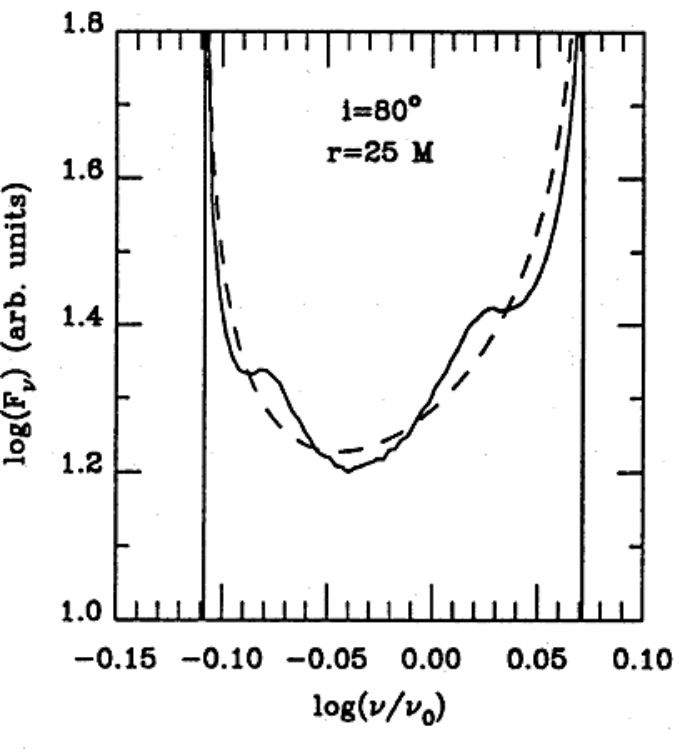
Figures 4 and 5 show two examples of “exact” (numerical) and approximated fitting of the profile of a line emitted by a ring around a black hole. For a low inclination () even close to the black hole () the numerical and approximate profiles are practically indistinguishable. However, even at relatively large distance from the hole () but high inclination () the imperfections of the approximate version of the flux are clearly visible.
The double-peaked line shape is, as in the newtonian case, due to the finite extent of the emission region, in this case a ring. The often used assumption will not produce double-peak lines if the outer emission region is not spatially limited.
4.7 Radiative structure
Here we will show an example of the solution for the vertical thin–disc structure which exhibits properties impossible to identify when the structure is vertically averaged. We will also consider here irradiated discs – such as AGN discs.
We write the energy conservation as :
| (108) |
where is the vertical (in the direction) radiative flux and is the viscous heating rate per unit volume. Eq. (108) states that an accretion disc is not in radiative equilibrium (), contrary to a stellar atmosphere. For this equation to be solved, the function must be known. As explained and discussed in Sect. 4.1 the viscous dissipation is often written as
| (109) |
Viscous heating of this form has important implications for the structure of optically thin layers of accretion discs and may lead to the creation of coronae and winds. In reality it is an ad hoc formula inspired by Eq. (29). We don’t know yet how to describe the viscous heating stratification in a real geometrically thin accretion disc and Eq. (109) just assumes that it is proportional to pressure. It is simple and convenient but it is not necessarily true.
When integrated over , the rhs of Eq. (108) using Eq. (109) is equal to viscous dissipation per unit surface:
| (110) |
where because of the integration from to while contains which is integrated from to (Eq. 26).
One can rewrite Eq. (108) as
| (111) |
where we introduced a new variable, the optical depth , being the Rosseland mean opacity and is the total optical depth. is of order unity.
At the disc midplane, by symmetry, the flux must vanish: , whereas at the surface, ()
| (112) |
Equation (112) states that the total flux at the surface is equal to the energy dissipated by viscosity (per unit time and unit surface). The solution of Eq. (111) is thus
| (113) |
where . Since , we have
| (114) |
To obtain the temperature stratification one has to solve the transfer equation. Here we use the diffusion approximation
| (115) |
appropriate for the optically thick discs we are dealing with. The integration of Eq. (115) is straightforward and gives :
| (116) |
The upper (surface) boundary condition is:
| (117) |
where is the irradiation temperature, which depends on , the albedo, the height at which the energy is deposited and on the shape of the disc. In Eq. (117) corresponds to the emergent flux and, as mentioned above, corresponds to the total flux () which explains the factor 1/2 in Eq (117). The temperature stratification is thus :
| (118) |
For the first term on the rhs has the form familiar from the stellar atmosphere models in the Eddington approximation.
In this case at one has .
Also for , the temperature at the disc midplane is
| (119) |
It is clear therefore that for the disc inner structure to be dominated by irradiation and the disc to be isothermal one must have
| (120) |
and not just as is sometimes assumed. The difference between the two criteria is important in X-ray binary and AGN discs since, for parameters of interest, (see Sect. 5.2).
4.8 Shakura-Sunyaev thin-disc solution
In their seminal and famous 1973 paper, Shakura & Sunyaev found power-law stationary solutions of the simplified version of the thin–disc equations presented in Sects. 4.1, 4.2 and 4.4. The 8 equations for the 8 unknowns , , , , , , and can be written as
Equations (ı) and (ıı) correspond to vertical structure equations (36) and (33), Eq. (vıı) is the radial Eq. (74), while Eq. (vııı) connects vertical to radial equations. Eq. (ııı) defines the sound speed, Eq. (ıv) is the equation of state and (vı) contains the information about opacities. The viscosity parametrization introduced in Shakura and Sunyaev, 1973 provides the closure of the 8 disc equations. Therefore they can be solved for a given set of , , and .
Power-law solutions of these equations exist in physical regimes where the opacity can be represented in the Kramers form and one of the two pressures, gas or radiation, dominates over the other. There are three regimes to be considered:
and
and
and .
Regimes and in which opacity is dominated by electron scattering will be discussed in Sect. 6. Here we will present the solutions of regime , i.e. we will assume that
| (121) |
The solution for the surface density , central temperature and the disc relative height (aspect ratio) are respectively
| (122) |
| (123) |
| (124) |
where , , and .
Since
| (125) |
the regime c.) solution exists only for radii
| (126) |
For this solution the viscous time is
| (127) |
so for the viscous time to be less than the age of the Universe (13.8 Gyr), for an Eddington accretion rate onto a black-hole, the outer disc radius must be , i.e. less than pc, or less than if in AGNs is .
In this solution it was assumed that the opacity is given by the formula
| (128) |
so that , for
| (129) |
Notice that is independent on the accretor’s mass.
It is characteristic of the Shakura-Sunyaev solution in this regime that the three , and radial profiles vary as . (This implies that the optical depth is constant with radius see Eq. vııı.) For high accretion rates and small radii, the assumption of opacity dominated by free-free and bound-free absorption will brake down, and the solution will cease to be valid. We will first consider the other disc end: large radii.
There, the temperature will finally drop () below K, the disc plasma will recombine leading to a drastic change in opacities which triggers a thermal instability.
5 Disc instabilities
In this section we will present and discuss the disc thermal and the (related) viscous instabilities. In AGN discs two instabilities are of interest: one is related to the hydrogen ionisation/recombination, the other occurs in discs where pressure is dominated by radiation. The instability is thermal when it grows on a thermal timescale, in a geometrically thin disc it means that the timescale is (see Eq. 59).
5.1 The thermal instability
A disc is thermally stable if the radiative cooling varies with temperature faster than the viscous heating. In other words a disc is thermally stable if
| (130) |
Using Eq. (119) one obtains
| (131) |
One can see from these equations that disc stability is determined by the temperature dependence of the opacities and that irradiation stabilises accretion discs.
5.1.1 Thermal instability due to hydrogen ionisation/recombination
In a gas–pressure dominated disc . At high temperatures (see Eq. 121). A thermal instability arises due to a rapid change of opacities with temperature when hydrogen begins to recombine (K) and this opacity dependence on temperature is no longer valid. In the instability region, the temperature exponent becomes large and positive: , and in the end cooling is decreasing with temperature.
Thus this thermal instability should be present in accretion discs with midplane temperature equal few times K and below. It has been established that it is at the origin of outbursts observed in discs around stellar-mass black-holes, neutron stars and white dwarfs. Systems containing the first two classes of objects are known as Soft X-ray transients (SXTs, where “soft” relates to their X-ray spectrum), while those containing white-dwarfs are called dwarf-novae (despite the name that could suggest otherwise, nova and supernova outbursts have nothing to do with accretion disc outbursts). This range of temperatures is also present in discs around AGNs and we will present its consequences in Sect. 5.3.
5.1.2 Thermal instability of radiation–pressure dominated discs
Radiation–pressure dominated () accretion discs are thermally unstable when the opacity is due to electron scattering on electrons. Indeed, in this case
| (132) |
because , while in a radiation pressure dominated disc
| (133) |
so that
| (134) |
and the disc is thermally unstable. This solution is represented by the middle branch with negative slope on the S-curve in Fig. 9 (see also Eq. 176) .
The presence of this instability in the model is one of the unsolved problems of the accretion disc theory because it contradicts observations which do not show any unstable behaviour in the range of luminosities where discs should be in the radiative pressure and electron-scattering opacity domination regime. This suggests that the disc description in this regime is incomplete.
For example, the radiation-pressure instability can be quenched if the disc vertical support is provided not by radiation but by a magnetic field. This field has to be brought into the disc from the surrounding medium, because the MRI dynamo is unable to produce a field with the required strength.
The heating rate can be rewritten as
| (135) |
and from
| (136) |
one deduces, as before, that a radiation-pressure dominated disc with electron-scattering opacity is thermally unstable.
However, with a magnetic-field pressure , introducing
| (137) |
one can write the heating rate as
| (138) |
from which one obtains
| (139) |
Radiative cooling is independent of the magnetic pressure, so for the heating rate no longer increases more rapidly with the central radiation pressure, than the cooling rate and the disc is thermally stable. It is not clear, however, how and from where a stabilising magnetic field will find itself in the right place and the right moment to quench the disc’s thermal instability (see a related discussion in Sect. 8).
5.2 Thermal equilibria: the -curve
We will consider thermal equilibria of an accretion disc in which heating is due only to local turbulence, neglecting the effects of irradiation, because in the case of AGN discs (contrary to discs in X-ray binaries) irradiation does not make much difference to the instability’s consequences. We put therefore .
The thermal equilibrium in the disc is defined by the equation (see Eq. 55), i.e. by
| (140) |
(Eq. 30). In general, is a function of density and temperature and in the following we will use the standard –prescription Eq. (21). The energy transfer equation provides a relation between the effective and the disc midplane temperatures so that thermal equilibria can be represented as a – relation (or equivalently a –relation). In the relevant range of temperatures () this relation forms an on the () plane as in Fig. 6. The upper, hot branch corresponds to the Shakura-Sunyaev solution presented in Section 4.8. The two other branches correspond to solutions for cold (partially ionised) discs. Near the upper bend of the and below it, convection can play an important role in the energy transfer.
Each point on the () -curve represents an accretion disc’s thermal equilibrium at a given radius, i.e. a thermal equilibrium of a ring at radius . In other words each point of the -curve is a solution of the equation. Points not on the -curve correspond to solutions of Eq. (55) out of thermal equilibrium: on the left of the equilibrium curve, cooling dominates over heating, ; on the right heating over cooling . Therefore a positive slope of the curve corresponds to stable solutions, since a small increase of temperature of an equilibrium state (an upward perturbation) on the upper branch, say, will bring the ring to a state where so it will cool down getting back to equilibrium. In a similar way a downward perturbation will provoke increased heating bringing back the system to equilibrium.
The opposite is happening along the -curve’s segment with a negative slope as both a temperature increase and decrease lead to a runaway. The middle branch of the -curve corresponds therefore to thermally unstable equilibria.
A stable disc equilibrium can be represented only by a point on the lower, cold or the upper, hot branch of the -curve. This means that the surface density in a stable cold state must be lower than the maximal value on the cold branch: , whereas the surface density in the hot stable state must be larger than the minimum value on this branch: . Both these critical densities are functions of the viscosity parameter , the mass of the accreting object, the distance from the center and depend on the disc’s chemical composition. In the case of solar composition the critical surface densities are
| (141) |
| (142) |
and the corresponing effective temperatures
| (143) |
| (144) |
where . Using the equation (see Eq. 75)
| (145) |
one obtains for the critical accretion rates
| (146) | |||
| (147) |
A stationary accretion disc in which there is a ring with effective temperature contained between the critical values of Eq. (143) and (144) cannot be stable. Since in a stationary disc, the effective temperature and the surface density both decrease with radius, the stability of a disc depends on the accretion rate and the disc size. For a given accretion rate a stable disc cannot have an outer radius larger than the value corresponding to Eq. (146).
A disc is hot and stable if the rate at which mass is brought to its outer edge () is larger than the critical accretion rate at this radius . On the other hand a disc is cold and stable if the mass–arrival rate to the disc is lower than the critical accretion rate at its inner radius .
Taking and , for black hole, an accretion disc will be unstable if the mass–arrival rate is contained in the range
| (148) | |||
| (149) |
or
| (150) |
This means that a typical accretion disc in an AGN is thermally unstable.
5.3 Variability of unstable AGN discs
The thermal instability at a certain disc’s radius produces a steep temperature gradient. This in turn creates a heating front which propagates radially bringing the cold disc regions to a hot state in which the heated up disc’s rings are on the upper branch of the -curve. The rise of temperature increases the viscosity (Eq. 23). In the discs around stellar-mass objects, such as white dwarfs, neutron stars and black holes, this process redistributes the mass of the disc, creating a quasi-stationary disc configuration with an accretion rate , the hot critical accretion rate at the outer disc radius. This corresponds to the outburst maximum, from which the accretion rate and luminosity decay because, by construction, in an unstable disc the mass-feeding rate is less than the hot critical accretion rate (see Eq. 148). When the accretion rate drops below this value, a cooling-front forms in the outer disc regions and propagates towards the center, bringing the disc behind it to a cold state, thus switching-off the outburst. During the following quiescence the disc, emptied during the outburst, fills-up again until it reaches somewhere the critical temperature, leading to the next outburst in the cycle. A typical dwarf-nova outburst or an X-ray binary transient event is characterised by a fast rise and slow decay which correspond to a viscous decay of a disc with a shrinking outer radius.
As can be seen in Figs. 7 and 8, which show the light-curve produced by an unstable disc around a supermassive black hole, the thermal disc instability produces outbursts also in AGNs, but a closer look shows that they are rather different from the eruptions observed in systems with less massive compact objects.
For relatively high mass-feeding rates ( – Fig. 7), the instability results in low-amplitude ( magnitude) outbursts corresponding to tiny modulations of the accretion rate. In fact, one sees that the timescale of brightness variations, corresponding to the temperature oscillations, is much shorter than the timescale of the accretion–rate variations. The basic reason for this is that the front propagation speed is approximately times the sound speed which means that front propagation time-scale is
| (151) |
where is the thermal time scale. Hence is shorter than the viscous time by a factor , i.e. by several orders of magnitude:
| (152) | ||||
| (153) |
The viscous time is therefore
| (154) |

Hence the front propagates so rapidly that the surface density does not have time to react to the changes of temperature.
In the case of stellar-mass compact objects, is shorter than , but not by such a large amount and strong gradients in the disk make the effective viscous time comparable to the front propagation time. The reason is that while in dwarf-nova stars and X-ray binaries the unstable disc region is at , in AGNs it is rather at , much deeper in the gravitational well of the accretor.
When one lowers the accretion rate to , the disc manages to descend to quiescence (Fig. 8), but it does it through a pure viscous decay, without a cooling front propagating down through the whole disc. The outburst phase lasts yr, which is roughly the disc viscous time. During this slow decay from maximum, heating/cooling fronts get reflected 400 times, creating as before low amplitude optical magnitude oscillations and tiny modulations of the accretion rate.
Neither disc irradiation, nor inner-disc truncation change basically the AGN outburst properties. This is not surprising since in stellar-mass systems, these effects play an important role mainly by affecting the cooling from propagation, which in the AGN case are of no importance.
It remains to be seen if in AGNs, thermal-instability outbursts occur in an observable way and even if they are occurring at all.
6 Beyond thin discs
Until now, we have assumed that accretion discs are thin, i.e. that . One of the consequences of this assumption was neglecting the advection terms in the energy and momentum equations for stationary accretion flows. The vertically averaged advective “cooling” term can be written as
| (155) |
where is a slowly varying function related to the entropy gradient and is usually . One then has
| (156) |
where we used Eqs. (56) and (74). Therefore neglecting the advective term in the energy equation
| (157) |
is justified if one assumes .
There are two regimes of parameters where this assumption is not valid, in both cases for the same reason: low radiative efficiency when the time for radial motion towards the black hole is shorter than the radiative cooling time. Low density (low accretion rate), hot, optically thin accretion flows are poor coolers and they are one of the two configurations were advection instead of radiation is the dominant evacuation-of-energy (‘‘cooling”) mechanism. Such optically thin flows are called ADAFs, for Advection Dominated Accretion Flows55 5 Some people prefer to call such flows RIAFs, from Radiatively Inefficient Flows but I prefer to stick to the name ADAF, which I had the pleasure to introduce.. Also advection dominated are high-luminosity flows, accreting at high rates, but they are called “slim discs” to account for their property of not being thin, but still being described as if this were not of much importance.
We shall start with optically thin flows.
- •
ADAFs
Advection Dominated Accretion Flows’ (ADAFs) is a term describing accretion of matter with angular momentum, in which radiation efficiency is very low. In their applications, ADAFs are supposed to describe inflows onto compact bodies, such as black holes or neutron stars; but very hot, optically thin flows are bad radiators in general so that, in principle, ADAFs are possible also in other contexts. Of course in the vicinity of black holes or neutron stars, the virial (gravitational) temperature is K, so that in optically thin plasmas, at such temperatures, both the coupling between ions and electrons and the efficiency of radiation processes are rather feeble. In such a situation, the thermal energy released in the flow by the viscosity, which drives accretion by removing angular momentum, is not going to be radiated away, but will be advected towards the compact body. If this compact body is a black hole, the heat will be lost forever, so that advection, in this case, acts as sort of a ‘global’ cooling mechanism. There, advection may act only as a ‘local’ cooling mechanism. (One should keep in mind that, in general, advection may also be responsible for heating, depending on the sign of the temperature gradient in some conditions, near the black hole, advection heats up electrons in a two-temperature ADAF).
In general the role of advection in an accretion flow depends on the radiation efficiency which in turns depends on the microscopic state of matter and on the absence or presence of a magnetic field. If, for a given accretion rate, radiative cooling is not efficient, advection is necessarily dominant, assuming that a stationary solution is possible.
- •
Slim discs
At high accretion rates, discs around black holes become dominated by radiation pressure in their inner regions, close to the black hole. At the same time the opacity is dominated by electron scattering. In such discs is no longer . But this means that terms involving the radial velocity are no longer negligible since . In particular, the advective term in the energy conservation equation (see Eq. 52) becomes important and finally, at super-Eddington rates, dominant. When the accretion flow is advection dominated and called a slim disc (Abramowicz et al., 1988).
- •
Windy discs
In a super-Eddington accreting disc, the radiative pressure can blow-out matter creating an outflow that will limit the luminosity to its local Eddington value. In such a case .
6.1 Advection–dominated–accretion–flow toy models
One can illustrate fundamental properties of ADAFs and slim discs with a simple toy model. The advection ‘cooling’ (per unit surface) term in the energy equation can be written as
| (158) |
(Eq. 155).
Using the (non-relativistic) hydrostatic equilibrium equation
| (159) |
one can write the advection term as
| (160) |
whereas the viscous heating term can be written as
| (161) |
where
| (162) |
Since ,
| (163) |
and, as said before, for geometrically thin discs () the advective term is negligible compared to the heating term and in thermal equilibrium viscous heating must be compensated by radiative cooling. Things are different at very high temperatures, when . Then the advection term is comparable to the viscous term and cannot be neglected in the equation of thermal equilibrium. In some cases this term is larger than the radiative cooling term and (most of) the heat released by viscosity is advected toward the accreting body instead of being locally radiated away as happens in geometrically thin discs.
From Eq. (74) one can obtain a useful expression for the square of the relative disc height (or aspect ratio):
| (164) |
Deriving Eq. (164) we used the viscosity prescription .
Using this equation one can write for the advective cooling
| (165) |
The thermal equilibrium (energy) equation is
| (166) |
The form of the radiative cooling term depends on the state of the accreting matter, i.e. on it temperature, density and chemical composition. Let us consider two cases of accretion flows:
-
optically thick
-
and
-
optically thin.
For the optically thick case we will use the diffusion approximation formula
| (167) |
and assume . With the help of Eq. (164) this can be brought to the form
| (168) |
For the optical thin case of bremsstrahlung radiation we have
| (169) |
which using Eq. (153) can be written as
| (170) |
- •
In the optically thick case we have therefore
(171) - •
In the optically thin case the energy equation has the form
(172)
There are two distinct types of advection dominated accretion flows: optically thin and optically thick. We will first deal with optically thin flows which are the true ADAFs.

6.1.1 Optically thin flows: ADAFs
For prescribed values and , Eq. (172) is a quadratic equation in whose solutions in the form of describe thermal equilibria at a given value of . Obviously, for a given this equation has at most two solutions. The solutions form two branches on the – plane:
- •
the ADAF branch
(173) and
- •
the radiatively–cooled branch
(174)
From Eqs. (173) and (174) it is clear that there exists a maximum accretion rate for which only one solution of Eq. (172) exists. This implies the existence of a maximum accretion rate at
| (175) |
This is where the two branches formed by thermal equilibrium solutions on the plane meet as seen on Figure 9.
The value of depends on the cooling mechanism in the accretion flow and the non-relativistic free-free cooling is not a realistic description of the emission in the vicinity () of a black hole. The flow there will most probably form a two-temperature plasma. In such a case , with almost no dependence on radius. For larger radii decreases with radius.
6.1.2 Optically thick flows: slim discs
Since the first two terms in Eq. (171) are the same as in (Eq. 172), the high , advection dominated solution is the same as in the optically thin case but now represents the
- •
Slim disc branch
(173) Now, the full equation (171) is a cubic equation in and on the plane its solution forms the two upper branches of the -curve shown in Fig. 9. The uppermost branch corresponds to slim discs while the branch with negative slope represents the Shakura-Sunayev solution in the regime a.) (see Sect. 4.8), i.e.
- •
a radiatively cooled, radiation-pressure dominated accretion disc
(176)
6.1.3 Slim discs and super-Eddington accretion
From Eqs. (164) and (176) one obtains for the disc aspect ratio
| (177) |
which shows that the height of a radiation dominated disc is constant with radius and proportional to the accretion rate.
But this means that with increasing advection becomes more and more important (see e.g. Eq. 163) and for
| (178) |
advection will take over radiation as the dominant cooling mechanism and the solution will represent a slim disc. Equation (178) can be also interpreted as giving the transition radius between radiatively and advectively cooled disc for a given accretion rate :
| (179) |
Another radius of interest is the trapping radius at which the photon diffusion (escape) time is equal to the viscous infall time
| (180) |
Notice that both and are proportional to the accretion rate.
In an advection dominated disc the aspect ratio is independent of the accretion rate:
| (181) |
therefore contrary to radiatively cooled discs, slim discs do not puff up with increasing accretion rate.
Putting (181) into Eq. (180) one obtains
| (182) |
Radiation inside the trapping radius is unable to stop accretion and since there is no limit on the accretion rate onto a black hole.
The luminosity of the toy-model slim disc can be calculated from Eqs. (168) and (173) giving
| (183) |
which implies . The luminosity of the slim–disc part of the accretion flow is then
| (184) |
where we used Eq. (179).
Therefore the total disk luminosity
| (185) | |||||
where is the luminosity of the radiation-cooled disc for which Eq. (75) applies.
Such logarithmic luminosity–accretion-rate dependence is observed in the inner regions of simulated accretion flows.
It is easy to see that the same luminosity formula is obtained when one assumes mass–loss from the disc, resulting in a radially variable accretion rate: (see Sect. 8).
7 Disc coronae
The X-ray emission observed from AGN accretion flows require the presence of emitters other than the optically thick accretion disc that we have described until now. The highest temperature one can get from the inner regions of such a disc is K (see Eq. 78). In analogy to solar and stellar coronae, the optically thin hot structures, much hotter than the underlying photosphere, the X-ray radiating structure in AGNs and other accreting compact body systems, is called a disc corona. The main idea is that the hot electrons of such a corona, inverse-Compton upscatter to high energies the soft photons emitted by the underlying disc.

There is not a single or even leading, or dominating disc corona model. Figure 10 shows various models or scenarios that have been proposed in the literature. Various models might correspond to various observed states of the accretion disc. The bottom configuration corresponds to the oldest proposed model whose idea was that differential rotation, together with convection and magnetic fields present in the disc, could produce loop-like structures, forming a magnetically-confined hot corona, in analogy to what is observed in the Sun. As for the Sun, magnetic-field reconnection could play a role in accelerating electrons to high energies. More recently, for different physical reasons (without invoking convection), models of magnetically heated coronae have been constructed. In this case it is the MRI amplification mechanism that, from the poloidal field, produces large amount of toroidal field in the upper layers of the disk.

Other models invoke accretion-disc “evaporation”, mechanism which, for low accretion rates, is supposed to produce ADAFs in the inner part of accretion discs. In fact an ADAF could play the role of a disc corona, as in the second panel from the top.
However, the most used “coronal” set-up is the so-called lamppost model, whose principle is shown in Figure 11. As it’s name demonstrate, this model does not have exaggerated ambitions to represent a physical reality, but is extremely useful when considering reverberation mapping. Of course this lamppost is a corona only in name. Most often one says that it could correspond to the base of a jet.
8 Discs, winds and jets
Accretion in AGN is the source of the inverse phenomenon: outflows (ejections) that with radiation are the key elements of the feedback cycle linking the supermassive central black hole to its host galaxy. Radiation and collimated outflows in form of jets interact with the interstellar medium leading to ejection or heating of the gas, but accretion disc winds play apparently the fundamental role in this interaction. Winds and collimated jets are produced by all systems containing a disc-accreting celestial body, from young stellar objects, through white dwarfs and neutron stars, to black holes of all masses, so one can expect that a common mechanism operates in accretion discs at all scales. The nature of this mechanism is still subject to controversy. In the case of winds, three possible mechanisms are invoked. Outer disc regions, most probably eject thermal-driven winds that are accelerated by the thermal gas pressure. Their velocity is at most km/s.
The radiative pressure due to the intense radiation of most AGN can be a very effective way to drive an accretion disc wind. For sub-Eddington accretion rates, UV absorption lines are the main source of opacity (as for winds of massive stars), while near the Eddington luminosity, Compton scattering is the wind blowing driver.
8.1 The “forgotten” Shakura-Sunyaev solution
In their seminal 1973 paper, Shakura and Sunyaev considered also the case of super-Eddington accretion and found a solution, alternative to the slim-disc solution (which they discarded). For mass-feeding rates , they identified the spherisation radius where the luminosity is close to the local Eddington value as
| (186) |
Then the solution is obtained by requiring that the local emission within nowhere exceeds its local Eddington limit, This will be true if the outflow is such that the accretion rate through the disc decreases as
| (187) |
Then the total luminosity is
| (188) |
(see Eq. 185). At very high accretion rates () the disc emission will be also strongly beamed by the flow geometry so that an observer situated in the beam of the emitting system will infer a luminosity
| (189) |
where is a beaming factor. Seen from the “side” such a source with very large apparent luminosities might appear as rather dim. On the other hand, if e.g., , a stellar mass ultra-luminous X-ray source (by definition erg/s) accreting at , seen along the beam, could have an apparent luminosity erg/s and look like an AGN, but will be positioned off the galactic center.
8.2 Relativistic jets
Magnetic fields may play a fundamental role in the production of disk winds. In this case the wind is accelerated by the centrifugal force of the magnetic field lines anchored on the disk and the magnetic pressure (Blandford-Payne mechanism, cf. Blandford and Payne, 1982). Magnetic fields are usually involved at the generation and acceleration phase and are always supposed to play a decisive role in keeping the jet collimated. Quite often in models, the jet is a collimated part of an outflow from the accretion disc but in other cases winds and jets can be launched by different mechanisms. Such a case is shown schematically in Fig. 12

where the relativistic jet is powered by the black-hole rotation while the source of the sub-relativistic wind energy is gravitational.
For launching relativistic jets observed in AGN, the best performing models involve large-scale magnetic fields anchored in the rapidly rotating matter of the inner parts of accretion discs. In the case of a rotating black hole two sources of jet launching energy are possible: the gravitational energy of accretion and the black-hole rotational energy that can be tapped through the electromagnetic Penrose process. This last mechanism is possible only when the accretor is a black hole because other rotating compact bodies do not have ergoregions.
The Blandford-Znajek (Blandford and Znajek, 1977, hereafter BZ) mechanism, which is the electromagnetic version of the Penrose process works on the same principle as its mechanical analogue: absorption of negative energy and negative angular momentum.

A typical jet–launching configuration is shown in Fig. 13, where one sees a poloidal magnetic field penetrating the black hole surface being twisted, forming a toroidal component. The power extracted by the BZ mechanism is equal to
| (190) |
where
| (191) |
is the magnetic flux threading one hemisphere of the black-hole horizon. is the area element in the plane. is numerical constant depending on the magnetic field geometry ( for the so-called split-monopole geometry, such as on Fig. 13. Quite often Eq. (190) is written with , which is a good approximation for black-hole spins up to , but for larger spins, of special interest when considering the BZ mechanism
| (192) |
is a more suitable approximation.
One defines the efficiency of the BZ mechanism as the ratio of the time-averaged electromagnetic flux extracting black-hole rotational energy to the averaged rate at which the black hole absorbs rest-mass energy:
| (193) | ||||
| (194) |
where
| (195) |
is the dimensionless magnetic flux threading the black hole.
Therefore the efficiency of the BZ mechanism depends strongly on the black-hole spin and on the magnetic flux threading the black hole surface. In Eq. (195) we have normalised by its observed interstellar-medium value. In the most efficient configuration the black hole receives as much large-scale magnetic flux as can be pushed into it by accretion. By supplying even more flux than this, some of it remains outside the horizon where it impedes the accreting gas, leading to a “magnetically arrested disc” (MAD; Tchekhovskoy et al., 2011). It is the MAD configuration that produces the most powerful relativistic jets.
This requires bringing this field to the innermost disc region where it is needed as an extractor of the black hole rotational energy. It’s far from obvious how this can be done.
The simplest problem to address in this context is to consider a poloidal field threading a Keplerian accretion disc. The turbulent-viscosity driven accretion tends to drag the field-lines inwards but due to resistivity they diffuse outwards. Numerical simulation of this problem have shown that the condition for the magnetic field lines to be significantly dragged inwards is
| (196) |
where , as before, is the kinematic viscosity coefficient, and
| (197) |
is the resistivity, with the electric conductivity. is known as the magnetic Prandtl number. The usual definition of the Prandtl number involves microphysical turbulence and viscosity, but here we are interested in transport coefficients of turbulent origin, hence the letter “t” in the index of the symbol. Therefore in thin accretion discs the magnetic field will be dragged inwards only for very large Prandtl numbers: , or . In MRI accretion discs , so “thick” discs, such as slim discs or ADAFs are needed if the magnetic flux is supposed to accumulate at the inner disc, near the black hole surface (Lubow et al., 1994).
Another possibility is that the disc’s angular momentum is not removed by turbulent viscosity, but by e.g., magnetic wind. Then Eq. (196) does not apply and the condition for field dragging becomes
| (198) |
In some models and , so field dragging is possible.
References
- Abramowicz et al., (1995) Abramowicz, M. A., Chen, X., Kato, S., Lasota, J.-P., and Regev, O. (1995). Thermal Equilibria of Accretion Disks. ApJLett, 438:L37.
- Abramowicz et al., (1988) Abramowicz, M. A., Czerny, B., Lasota, J. P., and Szuszkiewicz, E. (1988). Slim Accretion Disks. ApJ, 332:646.
- Abramowicz et al., (2010) Abramowicz, M. A., Jaroszyński, M., Kato, S., Lasota, J. P., Różańska, A., and Sądowski, A. (2010). Leaving the innermost stable circular orbit: the inner edge of a black-hole accretion disk at various luminosities. A&A, 521:A15.
- Balbus and Hawley, (1991) Balbus, S. A. and Hawley, J. F. (1991). A Powerful Local Shear Instability in Weakly Magnetized Disks. I. Linear Analysis. ApJ, 376:214.
- Bardeen and Petterson, (1975) Bardeen, J. M. and Petterson, J. A. (1975). The Lense-Thirring Effect and Accretion Disks around Kerr Black Holes. ApJLett, 195:L65.
- Blandford and Payne, (1982) Blandford, R. D. and Payne, D. G. (1982). Hydromagnetic flows from accretion disks and the production of radio jets. MNRAS, 199:883–903.
- Blandford and Znajek, (1977) Blandford, R. D. and Znajek, R. L. (1977). Electromagnetic extraction of energy from Kerr black holes. MNRAS, 179:433–456.
- Caballero-Garcia et al., (2019) Caballero-Garcia, M. D., Dovciak, M., Bursa, M., Papadakis, I., and Karas, V. (2019). X-ray Reverberation Observational Modelling in Active Galactic Nuclei. arXiv e-prints, page arXiv:1901.04357.
- Frank et al., (2002) Frank, J., King, A., and Raine, D. J. (2002). Accretion Power in Astrophysics: Third Edition.
- Gralla et al., (2019) Gralla, S. E., Holz, D. E., and Wald, R. M. (2019). Black hole shadows, photon rings, and lensing rings. PhysRevD, 100(2):024018.
- Hameury et al., (1994) Hameury, J. M., Marck, J. A., and Pelat, D. (1994). annihilation lines from accretion discs around Kerr black holes. A&A, 287:795–802.
- Hameury et al., (2009) Hameury, J. M., Viallet, M., and Lasota, J. P. (2009). The thermal-viscous disk instability model in the AGN context. A&A, 496(2):413–421.
- Hartle, (2003) Hartle, J. B. (2003). Gravity : an introduction to Einstein’s general relativity.
- Horne and Marsh, (1986) Horne, K. and Marsh, T. R. (1986). Emission line formation in accretion discs. MNRAS, 218:761–773.
- Jha et al., (2022) Jha, V. K., Joshi, R., Chand, H., Wu, X.-B., Ho, L. C., Rastogi, S., and Ma, Q. (2022). Accretion disc sizes from continuum reverberation mapping of AGN selected from the ZTF survey. MNRAS, 511(2):3005–3016.
- King, (2016) King, A. (2016). How big can a black hole grow? MNRAS, 456(1):L109–L112.
- Kotko and Lasota, (2012) Kotko, I. and Lasota, J. P. (2012). The viscosity parameter and the properties of accretion disc outbursts in close binaries. A&A, 545:A115.
- Lubow et al., (1994) Lubow, S. H., Papaloizou, J. C. B., and Pringle, J. E. (1994). Magnetic field dragging in accretion discs. MNRAS, 267(2):235–240.
- McKinney et al., (2012) McKinney, J. C., Tchekhovskoy, A., and Blandford, R. D. (2012). General relativistic magnetohydrodynamic simulations of magnetically choked accretion flows around black holes. MNRAS, 423(4):3083–3117.
- Paczyński, (2000) Paczyński, B. (2000). The Inner Boundary Condition for a Thin Disk Accreting Into a Black Hole. arXiv e-prints, pages astro–ph/0004129.
- Penrose, (1969) Penrose, R. (1969). Gravitational Collapse: the Role of General Relativity. Nuovo Cimento Rivista Serie, 1:252.
- Sadowski, (2011) Sadowski, A. (2011). Slim accretion disks around black holes. arXiv e-prints, page arXiv:1108.0396.
- Shakura and Sunyaev, (1973) Shakura, N. I. and Sunyaev, R. A. (1973). Black holes in binary systems. Observational appearance. A&A, 24:337–355.
- Shemmer et al., (2004) Shemmer, O., Netzer, H., Maiolino, R., Oliva, E., Croom, S., Corbett, E., and di Fabrizio, L. (2004). Near-Infrared Spectroscopy of High-Redshift Active Galactic Nuclei. I. A Metallicity-Accretion Rate Relationship. ApJ, 614(2):547–557.
- Sądowski et al., (2013) Sądowski, A., Narayan, R., Penna, R., and Zhu, Y. (2013). Energy, momentum and mass outflows and feedback from thick accretion discs around rotating black holes. MNRAS, 436(4):3856–3874.
- Starling et al., (2004) Starling, R. L. C., Siemiginowska, A., Uttley, P., and Soria, R. (2004). Constraints on active galactic nucleus accretion disc viscosity derived from continuum variability. MNRAS, 347(1):67–73.
- Tchekhovskoy et al., (2011) Tchekhovskoy, A., Narayan, R., and McKinney, J. C. (2011). Efficient generation of jets from magnetically arrested accretion on a rapidly spinning black hole. MNRAS, 418(1):L79–L83.
- Tetarenko et al., (2018) Tetarenko, B. E., Lasota, J. P., Heinke, C. O., Dubus, G., and Sivakoff, G. R. (2018). Strong disk winds traced throughout outbursts in black-hole X-ray binaries. , 554(7690):69–72.
- Toomre, (1964) Toomre, A. (1964). On the gravitational stability of a disk of stars. ApJ, 139:1217–1238.