SynGraphy: Succinct Summarisation of Large Networks via Small Synthetic Representative Graphs
Abstract
We describe SynGraphy, a method for visually summarising the structure of large network datasets that works by drawing smaller graphs generated to have similar structural properties to the input graphs. Visualising complex networks is crucial to understand and make sense of networked data and the relationships it represents. Due to the large size of many networks, visualisation is extremely difficult; the simple method of drawing large networks like those of Facebook or Twitter leads to graphics that convey little or no information. While modern graph layout algorithms can scale computationally to large networks, their output tends to a common hairball look, which makes it difficult to even distinguish different graphs from each other. Graph sampling and graph coarsening techniques partially address these limitations but they are only able to preserve a subset of the properties of the original graphs. In this paper we take the problem of visualising large graphs from a novel perspective: we leave the original graph’s nodes and edges behind, and instead summarise its properties such as the clustering coefficient and bipartivity by generating a completely new graph whose structural properties match that of the original graph. To verify the utility of this approach as compared to other graph visualisation algorithms, we perform an experimental evaluation in which we repeatedly asked experimental subjects (professionals in graph mining and related areas) to determine which of two given graphs has a given structural property and then assess which visualisation algorithm helped in identifying the correct answer. Our summarisation approach SynGraphy compares favourably to other techniques on a variety of networks.
1 Introduction
Network data is nowadays ubiquitous; social networks, protein networks and the Web are just a few examples of its spread. If network analysis is a crucial challenge to gain insights from such wealth of data, network visualisation represents an equally important aspect, especially because of its immediate usefulness to both network analysts and non-expert users; displaying (portions of) a network or structural properties (e.g. the degree distribution) makes more accessible the specific task at hand. The visualisation of small graphs poses no major problem; it can be achieved by graph drawing, i.e., placing each node of a graph at a specific position on the plane, and drawing edges as lines. The task then becomes to find suitable coordinates of nodes such that the drawing has judicious properties for the user (Purchase et al 1995), including the fact that connected nodes are near to each other, lines should not cross, points and lines should be uniformly distributed over the drawing area, and symmetries should be highlighted.
In data mining applications such as those arising on the web however, networks are so large that graph drawing is highly problematic, for at least two aspects. First, the computational cost associated to a certain graph drawing method which models properties like those listed above is usually high. Second, even if one comes up with a suitable algorithm, the drawing of very large graphs inherently leads to the “hairball effect”, i.e., the fact that all graphs look the same when drawn – see the article by Schulz and Hurter (Schulz and Hurter 2013) for a comprehensive overview about the topic. Examples of hairball-like plots are shown in Figure 1: even if the networks come from different domains, it is difficult to discern any of their structural properties.
To avoid the hairball effect, other methods are typically used, such as drawing only a part of the network (graph sampling), or aggregating its nodes into groups to show its main overall structural features (graph coarsening). These methods however lead to the problem of representativity, i.e., the sampled or coarsened graphs have structural properties differing from the original graphs. Some methods have been developed to bias graph sampling and coarsening algorithms to preserve certain graph properties (Cem et al 2013). However, these approaches are not focused on taking into account specific user’s information needs; they rely on the layout itself as a means to satisfy all information needs.
Contributions. In this paper we investigate the problem of visualising large graphs from the perspective of graph summarisation. Instead of applying sampling or coarsening, we devise an algorithm that generates synthetic graphs whose properties match that of the original graphs. The crucial aspect is that the syntactic graphs generated with our algorithm do not preserve any nodes or group of nodes from the original graphs; instead, they preserve the original structural and graph-theoretical properties. This allows us to reduce the problem of visualising large networks to the problem of drawing smaller, representative graphs instead of the original network. For a given input network, our algorithm SynGraphy performs the following steps: (i) it first measures several (and dynamically selectable) statistical properties of a network; (ii) scales them down to a given, small predefined number of nodes; (iii) generates a synthetic network with the required scaled-down statistical properties; and (iv) produces a graph drawing of the synthetic network using a classical graph drawing algorithm. The scaling down of statistics is trained on a large set of network datasets, in order to faithfully distinguish particularly low and high values of each network statistic. The summarisations of networks generated by our algorithm are evaluated in an experiment with human volunteers that are professionals in network analysis and related fields, asking them to estimate which of two given graphs has a higher or lower value of a given statistical property (e.g., clustering coefficient). SynGraphy performed well in comparison to plain graph drawing algorithms and graph sampling algorithms.
2 Related Work
The problem of graph visualisation is of primary importance in multiple fields of research, as many types of data can be modelled as networks. In order to visualise a graph, the most straightforward – and most common – method is to use graph drawing, i.e., producing a plot in which each node of the graph is represented as a point, and each edge as a line connecting a pair of points. Other, more advanced methods may try to show only a subset of a graph, or to summarise its properties in a specific way. The visualisation of network datasets can serve multiple purposes that can be clearly distinguished, and which lead to different visualisation methods:
- •
Exploration allows to explore nodes and edges of a graph. In the simplest case, a graph drawing allows to follow individual nodes and edges, as long as the graph is not too large. If the graph is large, a system of navigation may be used, in which one may click, for instance, on nodes to explore their neighbourhood;
- •
Structural properties – graph visualisation should allow to recognise structural properties of the graph drawn as a whole, e.g., whether the graph has a high clustering coefficient or not (van Ham et al 2009). This allows to perform other tasks such as comparing two networks, or finding an outlier in a given set of networks.
In this work the focus is on recognising structural properties: the goal is to allow both users and network analysts to recognise such properties in the graph visualisation, thus leading to the task of graph summarisation – the exploration of nodes and edges of the graph is then an orthogonal goal to ours.
2.1 Graph Drawing
Graph drawing, as opposed to graph visualisation, specifically refers to the task of laying out nodes and edges of a graph on a planar surface in order to produce a figure that shows the input graph as a whole. Graph drawing has also been called graph layouting and graph embedding. In general, graph drawing algorithms are based on optimising a certain cost or utility function, which models the quality of the graph drawing. Examples of features that can be incorporated are: drawing nodes near to their neighbours, avoiding crossing of edges, and avoiding multiple nodes at the same coordinates. A subset of such algorithms performs a force-directed layout, i.e., it simulates a physical force between nodes based on the physical model of springs connected the nodes. In very simple cases, these can be formulated as the eigenvectors of certain graph-characteristic matrices, in particular of the Laplacian matrix (Koren 2003). A well-known graph layout algorithm that is widespread in practice is the algorithm of Fruchterman and Reingold (Fruchterman and Reingold 1991), which bases its physical model on placing nodes near to its neighbours, but also on not placing nodes too near to each other – this makes the problem nonlinear and thus it cannot be expressed as eigenvectors of a matrix, but instead can be solved efficiently by direct optimisation algorithms, even if a global minimum of the energy function cannot always be found.
The obvious problem with pure graph drawing methods is that they don’t scale visually – if the number of nodes is too high, the resulting drawing will contain so many dots and lines that it will look like a single big patch of dots, without any recognisable network structure. This is the type of drawing that is usually called a “hairball”, and which is illustrated in Figure 1 using examples from the literature.
Another class of graph drawing algorithm approaches the problem from the point of view of wanting to draw the network such that certain particular properties of the network are highlighted, and thus choose to optimise the layout such that the given properties are made visible. An example from this class of algorithms is the hive plot (Krzywinski et al 2012), in which nodes of the given graph are assigned to one of three or more axes, which may be divided into segments. Nodes are ordered on a segment based on properties such as connectivity, density, centrality or quantitative annotations. The user then is free to choose whatever rules fit their data and visualisation requirements. Edges are drawn as curves. As we will see, the SynGraphy method presented in this paper has in common with hive plots that it makes it possible to assess network structure because both are based on network properties, not on aesthetic layout, making visualisations of two networks directly comparable.
2.2 Graph Summarisation
The inadequacy of drawing a complete graph when its size is too large leads to several methods in which the size of the input graph is reduced to obtain a smaller graph, which can then be drawn using any of the methods mentioned in the previous section. Such methods can be roughly divided into two types: (i) graph sampling techniques which choose a subset of the given graph’s nodes and edges, and (ii) graph coarsening techniques that aggregate the graph’s nodes into new nodes. These methods can be interpreted as graph summarisation: Automatic summarisation refers to the generation of shorter documents that summarise a given document, reducing it to the most important parts. Although the term summarisation has recently been applied to graphs, for instance by Liu and colleagues (Liu et al 2017), the term is, as of 2020, not common in the field.
Graph sampling. Graph sampling or graph sparsification refers to reducing a graph to a subset of its nodes and edges, with the goal of preserving certain graph properties. Simple graph sampling techniques perform a random sampling of nodes and edges, where each node or each edge is kept with a given probability (Hu and Lau 2013). In such methods, the expected properties of the resulting network can sometimes be derived in closed form. As an example, an edge sampling procedure that keeps each edge with probability will lead to a graph with clustering coefficient , where is the original graph’s clustering coefficient. On the other hand, certain graph sampling methods do not choose nodes and edges randomly, but use heuristics. For instance, an approach to filter a graph by removing edges in order of increasing betweenness centrality is described by Jia and colleagues (Jia et al 2008). The method preserves certain properties such as the connectivity, but there are still some features in the resulting graph that are hidden and cannot be identified for the entire graph.
Graph coarsening. Graph coarsening consists in aggregating multiple nodes of the input graph into a single node of the output graph, essentially performing vertex identification or edge contraction (Shawn et al 2011). As a result, high-level structural features such as connections between large communities are preserved, while information at the node level such as the clustering coefficient is usually lost. More examples (and drawings) of graph coarsening methods are given by Nocaj and colleagues (Nocaj et al 2015).
2.3 Graph Characteristics
In order to generate a graph with similar characteristics to an input graph, the characteristics of the latter need to be numerically quantified. This is achieved through the use of graph statistics, i.e., numerical measures of a graph. Graph statistics comprise the important class of subgraph counts, which count the number of occurrences of a particular small graph as a subgraph. For instance, the number of triangles is an often used graph statistic. The number of nodes and edges of a graph are subgraph counts too, corresponding to the subgraph consisting of a single node and a single edge respectively. Other graph statistics may be derived from subgraph counts, such as the clustering coefficient, which can be expressed as , where is the number of triangles and is the number of wedges, while other graph statistics are wholly unrelated to subgraph counts (e.g., the diameter). The graph statistics useful for the purposes of our algorithm, and described below, are summarised in Table 1. The input graph, as well as all other graphs used in this paper are undirected, without parallel edges, and loopless.
| Notation | Meaning |
|---|---|
| The input graph (potentially large) | |
| The output graph (to be drawn, small) | |
| Number of nodes | |
| Number of edges | |
| Number of wedges | |
| Number of claws | |
| Number of crosses | |
| Number of triangles | |
| Number of squares | |
| Average degree | |
| Clustering coefficient | |
| 4-Clustering coefficient | |
| Bipartivity | |
| Diameter | |
| Degree assortativity | |
| Scaled-down value of any statistic |
Network size and volume (). The number of nodes and edges in a network.
Number of wedges (). A wedge is a subgraph consisting of a central node connected to two other nodes. Equivalently, wedges are 2-stars or 2-paths, and their count can be expressed as
| (1) |
where is the degree of node .
Number of claws (). A claw is a subgraph equivalent to a 3-star.
Number of triangles (). A triangle is a subgraph consisting of three mutually connected nodes.
Number of squares (). A square is a group of four nodes connected to each other in the shape of a square, i.e., a cycle of length four.
Clustering coefficient (). The clustering coefficient represents the presence of a heightened number of triangles in the network (Newman 2003b), and can be expressed as
| (2) |
The clustering coefficient can take a value between zero and one, where the value one denotes that all possible triangles are present, and zero denotes a triangle-free network.
4-Clustering coefficient (). The 4-clustering coefficient is analogous to the clustering coefficient, but measures the probability that a randomly chosen path of length three is closed. It equals
| (3) |
where is the number of paths of length three. The 4-clustering coefficient complements the clustering coefficient, and may be used in bipartite or near-bipartite networks (Latapy et al 2008).
Bipartivity (). We use as a measure of bipartivity the ratio of the smallest and largest eigenvalue of the graph’s adjacency matrix (Kunegis 2015):
| (4) |
Average degree (). The average degree measures how many edges are connected to a node on average. The average degree is sometimes called the density. It equals .
Diameter (). The diameter of a network is the longest shortest distance between any two nodes. A distance is measured by the number of edges needed to reach one node from another.
Degree assortativity (). In some networks, the nodes with high degree are connected to other nodes with high degree, while nodes with low degree are connected to nodes with low degree. This is measured by the Pearson correlation coefficient, taken over all pairs of connected nodes (Newman 2003a).
3 The SynGraphy Approach
We are now ready to introduce our algorithm. Let be the large input graph that is to be summarised. Our algorithm proceeds in four steps:
- (i)
Compute the subgraph counts of
- (ii)
Scale down the subgraph counts
- (iii)
Generate with the scaled down subgraph counts
- (iv)
Generate a drawing of
Steps (i–iii) are described in the following subsections, while Step (iv) uses the algorithm by Fruchterman and Reingold (Fruchterman and Reingold 1991). For Step (ii), we describe two variants.
3.1 Scaling Down of Graph Statistics
The core idea of our algorithm to summarise the input graph is to generate a new graph with analogous structural properties to those of . Hence, the focus is on providing a meaningful rendering of ’s structural properties instead of ’s aesthetic. The size of , i.e., the number of nodes , can be chosen arbitrarily. For the sake of presentation, in what follows we set it to the value . As for the other statistics, their new values in the output graph need to be computed before can be generated. Certain graph statistics, such as the average degree and clustering coefficient are in principle scale-invariant, and could be simply carried over from without modification, i.e., it is possible to use and . Other statistics such as the number of triangles clearly scale with and their values have to be adjusted. In fact, the values of and may have to be adjusted too, as illustrated in Figure 2. In this light, we investigate two methods for determining the new values of these graph statistics:
- •
(NO): normalising all statistics empirically;
- •
(SI): use of statistics that by construction are independent of size.
Empirical Normal Distribution (NO). One possible assumption is that when normalised in certain ways, certain network statistics are size-independent. An example for this is the clustering coefficient. However, as we can derive empirically from actual network datasets, this is not entirely correct: the clustering coefficient does correlate with the size of the network, when measured in real-world networks, as shown in Figure 2. This observation leads to the following method for scaling down graph statistics: fit a distribution to the statistics of a set of known networks, and then read out the most likely values of the requested graph statistics, given the target size .
Given a set of real-world networks and a set of statistics, we compute the values of the statistics for all networks, and then fit a multivariate normal distribution to the data. The multivariate normal density is a generalisation of the univariate normal density to dimensions (Johnson and Wichern 2007). The -dimensional normal density of a -dimensional variable takes the form:
| (5) |
where the -vector is the mean of the distribution, the matrix the covariance matrix, and its determinant. The conditional probability distribution under a fixed is itself a multivariate normal distribution whose mean is given by
| (6) |
where the index denotes a restriction of the given quantity to the value corresponding to the size statistic , and denotes a restriction to all other columns and rows. Thus, for given statistic , the new value for the smaller graph is given by
| (7) |
Size-Independent Statistics (SI). Under the assumption that most subgraph counts can be expected to have values growing with the number of nodes in the network, the number of edges for instance can be written as
| (8) |
where is the average degree in the network. In a social network for instance, represents the average number of friends, and we can make the reasonable assumption that is independent from the network size, i.e., people don’t have more friends because the world is larger. Note that this assumption is not necessarily true, and the opposite case is taken into account in the previous paragraph. Assuming that is constant, it follows that we can use as a size-independent statistic, i.e., we can compute for the input graph, and then use .
Similarly, other subgraph counts can be derived to grow as powers of the network’s size, given an underlying graph model. In fact, this is true for whole classes of network models; in the Erdős–Rényi model for instance, the expected value of any subgraph count is a polynomial of the graph size (Ruciński 1988). For instance, the number of triangles in Erdős–Rényi graphs grows as the cube of the number of vertices.
For each subgraph count , we perform the following procedure: We derive the expected value of under suitable conditions, calling it ; and then derive from it the normalised statistic . Finally, we use , giving the new value of the plain subgraph count:
| (9) |
We now apply this method to individual subgraph count statistics. For each subgraph count statistic , we derive the expected value and the scaled down subgraph count statistic .
Number of edges (): Given a fixed average degree , we get
| (10) |
Number of wedges (): Given an average degree and an equal distribution of degrees, the expected number of wedges can be computed by noting that the number of wedges centred at each node is given by .
| (11) |
Number of claws and crosses (): Claws and crosses are 3-stars and 4-stars and as such, their expected values are analogous to those for 2-stars:
| (12) |
Number of triangles (): For the number of triangles, we assume a constant clustering coefficient . The clustering coefficient can be expressed by definition as . This gives
| (13) |
Number of squares (): This case is defined analogously to the number of triangles.
| (14) |
3.2 Graph Generation
As previously mentioned, graphs are generated by taking the fixed size of the network (), and corresponding scaled down values of six statistics including the count of edges, wedges, claws, crosses, triangles, and squares as obtained by applying the two methods (i.e., NO and SI) discussed above. The layout is drawn using the force-directed algorithm of Fruchterman and Reingold (Fruchterman and Reingold 1991).
The general form of our graph generation algorithm applying to any set of network statistics is given in Algorithm 1. The algorithm works by taking as a starting point an Erdős–Rényi graph with the correct number of nodes and edges, and then modifying the graph iteratively until the resulting graph is near enough to the target. At each step of the iteration, we need to consider a certain number of possible changes in the graph, and choose the change which leads to the lowest error measure. In order to compute the changes in the statistics efficiently, individual changes that are considered should be small, such that the changes in the statistic values can be easily computed. The smallest change that we can make in a graph (without changing the node set) is to add or remove an edge. In fact, the change in subgraph count statistics for the addition and removal of an edge can be expressed in terms of the immediate properties of the two involved nodes. Furthermore, in order to optimise the algorithm, the computation of the changes in statistics over all changes considered in one step makes use of common subexpression. Thus, we consider at each step the additions and removals of edges connected to one single node. As we show in the next section, this leads to efficient expressions for the change in the subgraph count statistics. We also note that the described algorithm, while performing the changes with best reduction in error at each step, is not a pure greedy algorithm; indeed, the algorithm continues to iterate in the case that the error cannot be further reduced by any single edge switch.
The function generates an Erdős–Rényi graph with vertices and individual edge probability . denotes the graph in which the state of the edge has been switched, i.e. removed or added depending on whether is present or not. The convergence parameter ensures that the expected ratio of nodes that were not visited since the last new minimum value was found equals . In all experiments, we use a value of .
Algorithm 1 requires to compute the difference in statistics between the current graph and the graph in which one edge is added or removed:
| (15) |
In order to speed up the algorithm, this calculation is performed in a vectorised way. The existence of closed-form expressions for decides whether a particular statistic can be used in our algorithm. Since must be computed at each step for all nodes (except for ), we give vectorised expressions that give a vector containing the value for all . The individual value computed for is then simply ignored. During the run of the algorithm, the graph is always represented by its symmetric adjacency matrix .
In what follows we provide expressions for the vectors measuring the change in statistic expressed as functions of the graph’s adjacency matrix , for each statistic . These expressions make use of the degree vector , which is updated along with the matrix . denotes the entry-wise product between two vectors and , and , the th column of .
Number of edges (): The number of edges will always increase or decrease by one, depending on the previous state of the edge .
| (16) |
Number of wedges (): When adding an edge, the number of wedges increases by the sum of the degrees of the two connected nodes. When removing an edge, the number of wedges decreases by the sum of the degrees of the two nodes, minus two.
| (17) |
Number of claws (): When the two nodes and are not connected, the number of added claws equals . When the two nodes are connected, the number of removed wedges can be computed in the same way, but based on the degrees after the removal.
| (18) | |||
Number of crosses (): The expression for the number of -stars for higher follows the same pattern as for and . Due to the asymmetry between the addition and the removal of edges, the resulting expressions get increasingly complex.
| (19) | |||
Number of triangles (): When adding an edge between two nodes, the number of added triangles equals the number of common neighbours between the two nodes. Likewise when removing an edge, the number of removed triangles equals the number of common neighbours of the two nodes. We thus get the following expression for the change in the number of triangles.
| (20) |
We thus need to perform one sparse matrix-vector multiplication for each iteration step.
Number of squares (): To compute the number of squares added or removed, we count the number of paths of length three added or removed between and . In principle, this can be achieved by using the expression for and multiplying once more by . However, this will also include the number of paths of length three that include an edge or multiple times, or that include the edge if it is present. Thus, these cases must be subtracted to get the correct number of squares added or removed.
| (21) |
We thus need to perform two matrix-vector multiplications in this step.
4 Experimental Evaluation
In this section, we describe the user experiments conducted in order to evaluate the two proposed graph visualisation methods against baseline methods, as well as evaluate the runtime of SynGraphy empirically, and perform an experiment to determine the influence of the size of the generated graphs on the drawings.


 FR
LA
SU
FR
LA
SU


 SN
NO
SI
SN
NO
SI
4.1 Experimental Setup
The human experiment was conducted via a website11 1 The site was available at http://nohairball.west.uni-koblenz.de/, and is offline as of this writing. on which practitioners in the fields of graph mining, network analysis, and related fields were asked to participate. After showing the participants the definitions of the graph statistics
as defined in Section 2.3, each participant is shown, in turn, twelve pages organised as follows. After choosing one graph visualisation method at random (see list in Table 2), two networks are chosen at random from a set of 18 predefined networks, and visualised using the chosen method. Then, a graph statistic is chosen at random from the set of the seven mentioned graph statistics; the participant is asked to determine which of the two shown graphs has a higher or lower value for the given graph statistic. The layout of the page (which graph is shown left and right), and whether the question is formulated as higher or lower is chosen randomly. The user may also determine that she cannot determine the difference by clicking on a button for that purpose. The users’ answers are logged, and evaluated in the following. The participants in the experiments were mostly from a computer science and network science background, partly associated with the authors’ institution, and partly external.
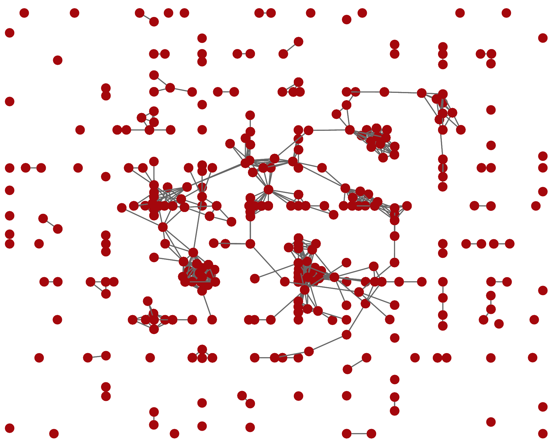
The experiment’s web page was available in mid 2016, and was disseminated using various channels. An anonymised screenshot of the experiment running in a browser is shown in Figure 4. For reference, Figure 3 shows a single network dataset visualised with all six algorithms used in the experiments.
| Method | |
| FR | Fruchterman–Reingold (Fruchterman and Reingold 1991) |
| LA | Laplacian embedding (Koren 2003, see e.g.) |
| SU | Uniform vertex sampling1 |
| SN | Node sampling1 |
| NO | SynGraphy with empirical statistic distribution1 |
| SI | SynGraphy with size-independent statistics1 |
| 1These methods are followed by the use of the Fruchterman–Reingold method for drawing the resulting small graph. | |

The experiment was divided into two parts. In the first part, we show to the experimental subject the definitions of the various network properties and show two example graphs with high and low values of each properties. In the second part, some random graphs (generated using the methods discussed above) were shown to the users. The user had to identify the graph with a low or high value of a certain property. The six graph visualisation methods used in the experiment are given in Table 2. For the uniform vertex sampling method, we chose a random subset of the nodes, and keep all edges connected to at least one of them (Clauset 2014; Hu and Lau 2013). For node sampling, we chose a random subset of all nodes, and keep all edges connecting two of them.
4.2 Results
From the logs of the experiments, we determine for each page view whether the person was correct or incorrect in their assessment of the given network statistic for the two given graphs visualised with the given method. In total, 3,049 questions where answered by 79 unique identified participants, plus an unknown number of anonymous participants.22 2 Participants were given the possibility to optionally enter their name into the system. Each question is thus answered in exactly one of three ways: correct, incorrect, or skipped. Thus, we collect three counts:
- •
, the number of correct answers,
- •
, the number of incorrect answers,
- •
, the number of skipped answers.
The total number of questions shown is then . From these numbers, we compute the success rate and the confusion rate as follows:
| (22) |
Success Rate by Visualisation Method. Figure 5 shows the overall success rate for each graph visualisation method used in the experiment, including the two SynGraphy variants. The result shows that the overall success rate of the SynGraphy variant based on normalisation (NO) is significantly higher than all the other methods used in the experiment ( test, ). The SynGraphy variant based on statistics that are by construction independent of size (SI) does not show statistically better results than the node sampling (SN) method ( test, ) and the uniform vertex sampling (SU) method ( test, ). The fact that the empirical normalisation method (NO) performs much better than the one using predetermined normalised statistics (SI) is also enlightening, as it suggests that statistics such as the clustering coefficient, which are size-independent in theory by construction, are not necessarily so in practice, and that in practice it is more effective to normalise subgraph count statistics using available empirical data from actual network datasets.
Success Rate by Network Statistic. Comparing the individual network statistics with each other, it appears that the task of identifying structural network properties is, as a general rule, a difficult one. As seen in Figure 6, only a single statistic reaches an overall success rate (over all visualisation methods combined) of more than 50%, this being the clustering coefficient. This may be explained by the better knowledge of the clustering coefficient of many participants, who, despite the explanations given at the start of the experiments, may not be familiar with less well-known network statistics such as the degree assortativity, and may thus have a harder time recognising it in graph drawings. It can also be observed that non-normalised statistics such as the raw number of wedges () have low success rates – justifying the need for normalised statistics such as the clustering coefficient.
Confusion Rate. In Figure 5, we may also compare the confusion rate of the different graph visualisation methods. The interpretation of the confusion rate is ambivalent: A high confusion rate may indicate that a particular graph visualisation method is confusing for the user, but at the same time a graph visualisation method should avoid misleading users – it is better if the user is undecided, than for her to be wrong. Thus, the confusion rate should not be taken as an indicator of the quality of a graph visualisation method, but rather as a measure of how convincing the resulting plots look. Thus, a graph visualisation method with a low confusion rate may lead to the user often thinking that they are able to recognise the properties of the graph, regardless of whether they are right or wrong. That being said, the smallest confusion rates are achieved by the two sampling methods (SU, SN), and the highest by the direct drawing methods (FR, LA). The two SynGraphy variants then achieve an intermediate confusion rate. To be precise, the size-independent SynGraphy (SI) method has a significantly lower confusion rate than the Fruchterman–Reingold (FR) method ( test, ), and also than the four baseline methods combined ( test, ).
Individual Results. The results shown in Figure 7 allow us to make more detailed remarks about the performance of the individual graph visualisation methods with respect to individual network statistics. We observe that the SynGraphy variant based on empirically derived normalisation (NO) gives the highest success rate for the number of claws and density, while for other network statistics, other visualisation methods than SynGraphy perform better, although no single one is better for many network statistics. In particular, the plain Fruchterman–Reingold method has the highest success rate for the number of wedges and squares, the Laplacian embedding has the highest success rate for the diameter, uniform vertex sampling has the highest success rate for the clustering coefficient and assortativity, and finally node sampling has the highest success rate for the bipartivity coefficient. Thus, it seems that if a graph visualisation is needed in which a particular network property should be emphasized, then we cannot claim that the SynGraphy method is the best choice in all cases. It should also be noted that if a particular property such as bipartivity is to be emphasized, then other, more specific methods may be chosen.
4.3 Runtime Experiments
In order to assess the runtime of the method empirically, we show the runtime of the SynGraphy algorithm in Figure 8. The two variants of SynGraphy have, for all practical purposes, the same runtime, as they differ only in the step of scaling down the network statistics, whose runtime is constant and very small, i.e., it does not depend on the network size. The amount of memory taken up by a sparse graph is proportional to the number of edges rather than the number of nodes, and thus we measure the runtime in function of the number of edges, i.e., the graph’s volume .
We can derive the runtime of the SynGraphy algorithm in function of the input graph’s volume as follows. The different steps of the algorithm are in turn: (i) computation of subgraph counts, (ii) scaling down of subgraph counts, (iii) generation of the synthetic graph, and (iv) generation of the graph layout using the Fruchterman–Reingold algorithm. Steps (ii–iv) have runtime independent of the graph’s number of edges , as they are performed on data of fixed size, and thus have a formal runtime of . Step (i), the counting of subgraphs, is the only part of the algorithm depending on , and its actual runtime is dominated by the computation of the counting of squares (4-cycle subgraphs), which is quadratic. Thus, the overall runtime of SynGraphy is expected on theoretical grounds to be . The empirical data as shown in Figure 8 is consistent with that runtime of .
4.4 Varying
In order to assess the influence of the size of the generated small synthetic graphs on the quality of the summarisation, we generate graph summarisations for varying using a single network, the email network of Enron (Klimt and Yang 2004) already used in Figure 1, visualised using the SynGraphy variant based on the empirically learned normal distribution of statistics (NO). The resulting graphs are shown in Figure 9, for varying between a value of up to a value of .
We observe that for very small , the small number of drawn nodes and edges is not enough to convey any meaningful information about the network, and thus the summarisation of the original graph is not a useful representation of the original network. For too large values of , the drawn graphs approach a “hairball”-like image, and thus they too are not useful representations of the graph to be summarised. Intermediate values in the approximate range give an acceptable trade-off between the two conditions, leading us to recommend a value of 80 for . This is also the value used in the previous experiments, as explained in the previous section.
5 Discussion
We have seen that in the overall evaluation the proposed SynGraphy variant based on the empirical distribution of graph statistics (NO) has the highest success rate of all tested visualisation methods, and we may thus recommend it as a first step in the analysis of networked data. However, if certain specific graph properties are to be emphasized, then traditional graph drawing methods may be best instead – our experiments showed for instance that a Laplacian embedding is well suited to making evident the diameter of a graph. We must of course stress that this method is only useful if general, structural properties are to be summarised – an exploration of the actual nodes and edges of the network is, by construction, not possible with graph summarisation methods. The problem of visualising the individual nodes and edges of a given large network is a separate problem that, in the end, cannot be solved without showing only a small subset of the given network, giving rise to the problem of letting the user search the nodes of a graph, for instance using a search engine or even a recommender system, if the nodes of the graph are amenable to that – that problem is however clearly outside of the scope of graph summarisation.
Finally, we should address the question whether graph visualisation and summarisation are a necessary part of the graph mining process. If certain specific properties such as the bipartivity or assortativity of a given network are to be detected, it is usually more productive to simply compute and show the corresponding numerical statistics. Graph visualisation and summarisation however are usually used for a higher-level purpose: As recently shown (Matejka and Fitzmaurice 2017), a general-purpose visualisation of a given dataset is often a simple and effective way of starting an in-depth analysis. Network datasets are of course not exempt from this, and thus a graph summarisation method such as SynGraphy can be recommended to fill that role, and, as we showed in our experimental evaluation, give practitioners a better idea of a given network dataset’s overall structural properties.
An evident future extension of our method is to apply it to further graph properties, although with more elaborate graph statistics, the task of graph generation becomes more runtime-intensive, as the vectorised expressions as given in Section 3.2 are then not possible anymore.
References
- Cem et al (2013) Cem E, Tozal ME, Sarac K (2013) Impact of sampling design in estimation of graph characteristics. In: Proc. Perform. Comput. and Commun. Conf., pp 1–10
- Clauset (2014) Clauset A (2014) Network analysis and modeling, small worlds and navigable networks. Lecture notes
- Fruchterman and Reingold (1991) Fruchterman TMJ, Reingold EM (1991) Graph drawing by force-directed placement. Software: Pract and Exp 21(11):1129–1164
- van Ham et al (2009) van Ham F, Schulz HJ, Dimicco JM (2009) Honeycomb: Visual analysis of large scale social networks. In: Proc. Conf. Human-Computer Interaction, pp 429–442
- Harrigan (2014) Harrigan M (2014) A network analyst’s view of the block chain. http://www.coindesk.com/network-analysts-view-block-chain/
- Hu and Lau (2013) Hu P, Lau WC (2013) A survey and taxonomy of graph sampling. CoRR abs/1308.5865
- Jia et al (2008) Jia Y, Hoberock J, Garland M, Hart JC (2008) Visualization of social and other scale-free networks. Trans Visualization and Computer Graphics 14(6):1285–1292
- Johnson and Wichern (2007) Johnson RA, Wichern DW (2007) Applied Multivariate Statistical Analysis, 6th edn. Pearson
- Joshi-Topé et al (2005) Joshi-Topé G, Gillespie M, Vastrik I, D’Eustachio P, Schmidt E, de Bono B, Jassal B, Gopinath G, Wu G, Matthews L, Lewis S, Birney E, Stein L (2005) Reactome: A knowledgebase of biological pathways. Nucleic Acids Res 33(Database):D428–D432
- Klimt and Yang (2004) Klimt B, Yang Y (2004) The Enron corpus: A new dataset for email classification research. In: Proc. Eur. Conf. on Mach. Learn., pp 217–226
- Koren (2003) Koren Y (2003) On spectral graph drawing. In: Proc. Int. Comput. and Comb. Conf., pp 496–508
- Krzywinski et al (2012) Krzywinski M, Birol I, Jones SJM, Marra MA (2012) Hive plots – rational approach to visualizing networks. Brief Bioinform 13(5):627–644
- Kunegis (2013) Kunegis J (2013) KONECT – The Koblenz Network Collection. In: Proc. Int. Conf. on World Wide Web Companion, pp 1343–1350
- Kunegis (2015) Kunegis J (2015) Exploiting the structure of bipartite graphs for algebraic and spectral graph theory applications. Internet Math 11(3):201–321
- Latapy et al (2008) Latapy M, Magnien C, Vecchio ND (2008) Basic notions for the analysis of large two-mode networks. Soc Netw 30(1):31–48
- Liu et al (2017) Liu Y, Dighe A, Safav T, Koutra D (2017) Graph summarization: A survey. ACM Comput Surv In review
- Matejka and Fitzmaurice (2017) Matejka J, Fitzmaurice G (2017) Same stats, different graphs: Generating datasets with varied appearance and identical statistics through simulated annealing. In: Proc. Conf. on Human Factors in Comput. Syst., pp 1290–1294
- Newman (2003a) Newman MEJ (2003a) Mixing patterns in networks. Phys Rev E 67:026,126
- Newman (2003b) Newman MEJ (2003b) The structure and function of complex networks. SIAM Rev 45(2):167–256
- Nocaj (2015) Nocaj A (2015) Untangling networks: Focus on less to see more. PhD thesis, Univ. of Konstanz
- Nocaj et al (2015) Nocaj A, Ortmann M, Brandes U (2015) Untangling the hairballs of multi-centered, small-world online social media networks. J of Graph Algorithms and Appl 19(2):595–618
- Purchase et al (1995) Purchase HC, Cohen RF, James M (1995) Validating graph drawing aesthetics. In: Proc. Graph Drawing Symp., pp 435–446
- Redmond and Cunningham (2013) Redmond U, Cunningham PD (2013) A temporal network analysis reveals the unprofitability of arbitrage in the Prosper marketplace. Expert Syst with Appl: An Int J 40(9)
- Ruciński (1988) Ruciński A (1988) When are small subgraphs of a random graph normally distributed? Prob Th Rel Fields 78:1–10
- Schulz and Hurter (2013) Schulz HJ, Hurter C (2013) Workshop: Grooming the hairball – how to tidy up network visualizations? In: Proc. Inf. Vis. Conf.
- Shawn et al (2011) Shawn M, Brown WM, Klavans R, Boyack KW (2011) OpenOrd: An open-source toolbox for large graph layout. In: Proc. Vis. and Data Anal.