A GPU-Parallelized Interpolation-Based Fast Multipole Method for the Relativistic Space-Charge Field Calculation

The space-charge effect is one of the most important topics in the study of beam physics. In recent years, the fast multipole method (FMM) has attracted increasing attention in the numerical modeling of the space-charge field [1, 2, 3, 4, 5]. Compared to the particle-in-cell (PIC) method [6, 7, 8, 9, 10] which has been a standard choice in the community of accelerator physics for decades, the FMM has the following advantages in the context of the study of beam physics:

1. 1.

   Through the point-to-point (P2P) operation, FMMs inherently consider the point-to-point Coulomb effects, e.g., disorder-induced heating and the Boersch effect which are non-negligible in the simulation for cold and dense beams [4].

2. 2.

   The FMM is a gridless algorithm and can effectively handle charged particle beams with complex geometry [2].

There have been many efforts using FMM for the modeling of electrostatic Coulomb interactions [11, 1, 4, 3]. The electrostatic model is suitable for the study of non-relativistic particle beams, e.g., the simulation of ultrafast electron microscopy [1, 4] and the simulation of proton dynamics in synchrotrons [11]. However, for the modeling of energetic electron beams, the consideration of the relativistic effect on the particle field may be essential. One approach to include relativistic effects is the quasi-electrostatic model [12, 5] where all particles are assumed stationary in a rest-frame of the particle beam. The electrostatic field on each particle is first solved in the rest-frame and the corresponding field in the lab-frame is calculated through the Lorentz transformation [8, 13]. Because of the assumption made in the quasi-electrostatic model, some adjustments are necessary to incorporate the effect of the momentum spread. For example, to handle particle beams with larger energy spread, a technique called energy-binning was proposed by binning particles in energy; the total space-charge field comes from the superposition of the source particle field evaluated in the rest-frame of each bin [14, 15]. This study is the extension of our previous work on treecode [16] and consists of two parts. In the first part (Sections 2–6), we formulate an FMM for the efficient computation of the relativistic space-charge field. Our formulation is based on the barycentric Lagrange dual tree traversal (BLDTT) proposed in Ref. [17]. BLDTT uses barycentric Lagrange interpolation for the kernel approximation and dual tree traversal for the construction of interaction lists. Different from the quasi-electrostatic model, the proposed FMM is formulated in the lab-frame and can be applied without the use of the Lorentz transformation. We first introduce the idea of an interpolation-based FMM. After that, we formulate an interpolation-based FMM for the computation of the relativistic space-charge field. In particular, we derive a modified admissibility condition for the cluster-cluster interaction of the relativistic kernel used in the formulated FMM. The algorithms and the implementation details associated with the proposed FMM are also provided. The second part of this study (Sections 8–11) is devoted to the GPU parallelization of the proposed FMM. Different to Ref. [17] which is based on OpenACC (a directive-based programming model) [18], our parallelization is based on the CUDA programming model. We discuss the data structure and the design issues in the implementation of the GPU parallelization. A package containing serial and GPU-parallelized solvers is implemented in the Julia programming language. The performance of the parallel solver is also demonstrated.

In this section, we give a short overview of the interpolation-based FMM [19, 17]. Consider two particle-clusters $S_{t}$ and $S_{s}$. The total force-field $f$ from the source particles in the cluster $S_{s}$ applied on a target particle with index $i$ and position $\bm{x}_{i}\in S_{t}$ through an interaction kernel $g(\bm{\cdot,\cdot})$ can be modeled as

Here and in the following, $\widehat{S}_{t}$ and $\widehat{S}_{s}$ represent the index sets of the particles in $S_{t}$ and $S_{s}$, respectively. The symbol $m_{j}$ is the physical quantity of the source particle with index $j$. Although the actual meaning of $m_{j}$ depends on the physics problem we investigate, without loss of generality, we call it mass throughout this section.

The idea of FMM for a fast evaluation of the summation in (2.1) is based on an approximation of the kernel function by interpolating both the target variable $\bm{x}_{i}$ and the source variable $\bm{x}_{j}$

Here, we define the bounding box $Q$ of a cluster $S$ as

with $a_{g}=\min_{i\in\widehat{S}}\{g\}$, $b_{g}=\max_{i\in\widehat{S}}\{g\}$ and $g\in\{x,y,z\}$. The Lagrange basis polynomials over the bounding boxes of $S_{t}$ and $S_{s}$ are defined as

with the corresponding interpolation points

Substituting (2.2) into (2.1), we have

By observing (2.3), we identify the four of FMM kernels:

• •

  P2M (point to multipole): the micro particles in the cluster $S_{s}$ are aggregated into a few macro particles and the mass of each macro particle ($M_{S_{s},\bm{\nu}}$, also called multipole) can be computed by

  $$M_{S_{s},\bm{\nu}}:=\sum_{j\in\widehat{S}_{s}}\ell_{S_{s},\bm{\nu}}(\bm{x}_{j})m_{j}.$$

  (2.4)

• •

  M2L (multipole to local): the multipoles of the source cluster are used to evaluate the force-fields acting on the macro particles ($L_{S_{t},\bm{\mu}}$, also called local field) in the target cluster $S_{t}$

  $$L_{S_{t},\mu}:=\sum_{\bm{\nu}}\bm{g}(\bm{\xi}_{S_{t},\bm{\mu}},\bm{\xi}_{S_{s},\bm{\nu}})M_{S_{s},\bm{\nu}}.$$

  (2.5)

• •

  L2P (local to point): in the target cluster, the effective force-fields acting on the macro particles are transferred to the micro particle at $\bm{x}_{i}$ by

  $$f(\bm{x_{i}})=\sum_{\bm{\mu}}\ell_{S_{t},\bm{\mu}}(\bm{x}_{i})L_{S_{t},\bm{\mu}}.$$

  (2.6)

• •

  P2P (point to point): if $S_{t}$ and $S_{s}$ do not fulfill an admissibility condition (ADMC, also called multipole acceptance criteria MAC in some literature [20, 21]) so that (2.2) is not applicable, the force-field can be calculated directly by

  $$f(\bm{x}_{i})=\sum_{j\in\widehat{S}_{s}}g(\bm{x}_{i},\bm{x}_{j})m_{j}\quad\forall i\in\widehat{S}_{t}.$$

  (2.7)

  This also applies for the case $S_{t}=S_{s}=S$, where $i,\,j\in\widehat{S}$ and $i\neq j$.

One main feature of the FMM is the consideration of the cluster-cluster interaction (M2L) through macro particles; and hence, the total number of operations for the evaluation of force-fields can be drastically reduced. In the FMM, we first partition all particles in the system into a hierarchy of clusters (cluster tree). If we directly use (2.4) to compute the multipole of each cluster, the number of operations for computing the multipoles of the whole cluster tree is

with the assumption that the number of macro particles used for the approximation and the number of micro particles contained in the leaf cluster are both $N_{r}$. To reduce the total number of operations for computing the multipoles, we can make use of the following property of polynomial interpolation stated in Theorem 1.

This equality can be seen by the fundamental theorem of algebra since both LHS and RHS have the same values at the $n+1$ points $\{\xi_{S,k}\mid k=0,\ldots,n\}$ and the RHS is a polynomial of degree $n$. By using Theorem 1, we can introduce two further procedures and two kernels of FMM:

• •

  Upward Pass: a source particle cluster $S$ is subdivided into a hierarchy of clusters of the depth $\kappa$ (called cluster tree [22, 23]) . The multipoles of each cluster can be computed by the multipoles of its children clusters in view of

  	$\displaystyle M_{S,\bm{\nu}}$	$\displaystyle=\sum_{j\in\widehat{S}}\ell_{S,\bm{\nu}}(\bm{x}_{j})m_{j}$
  		$\displaystyle=\sum_{s^{\prime}\in\text{children}(S)}\sum_{j\in\widehat{s^{\prime}}}\ell_{S,\bm{\nu}}(\bm{x}_{j})m_{j}$
  		$\displaystyle\stackrel{{\scriptstyle\mathchoice{\hbox to0.0pt{\hss$\displaystyle{\eqref{eq:interpolation_of_polynormial}}$\hss}}{\hbox to0.0pt{\hss$\textstyle{\eqref{eq:interpolation_of_polynormial}}$\hss}}{\hbox to0.0pt{\hss$\scriptstyle{\eqref{eq:interpolation_of_polynormial}}$\hss}}{\hbox to0.0pt{\hss$\scriptscriptstyle{\eqref{eq:interpolation_of_polynormial}}$\hss}}}}{{=}}\sum_{s^{\prime}\in\text{children}(S)}\sum_{j\in\widehat{s^{\prime}}}\sum_{\bm{\nu}^{\prime}}\ell_{S,\bm{\nu}}(\xi_{s^{\prime},\bm{\nu}^{\prime}})\ell_{s^{\prime},\bm{\nu}^{\prime}}(\bm{x}_{j})m_{j}$
  		$\displaystyle=\sum_{s^{\prime}\in\text{children}(S)}\sum_{\bm{\nu}^{\prime}}\ell_{S,\bm{\nu}}(\xi_{s^{\prime},\bm{\nu}^{\prime}})\sum_{j\in\widehat{s^{\prime}}}\ell_{s^{\prime},\bm{\nu}^{\prime}}(\bm{x}_{j})m_{j}$
  		$\displaystyle=\sum_{s^{\prime}\in\text{children}(S)}\sum_{\bm{\nu}^{\prime}}\ell_{S,\bm{\nu}}(\xi_{s^{\prime},\bm{\nu}^{\prime}})M_{s^{\prime},\bm{\nu}^{\prime}}.$		(2.9)

  Equation (2.9) is the formula of the M2M (multipole to multipole) kernel. In FMM, the multipoles of the source cluster tree are updated by a procedure called upward pass. In the upward pass, the multipoles of the leaf clusters are first evaluated with P2M (2.4); and then, we start from the second deepest level of the cluster tree (i.e., level $\kappa-1$) and apply M2M (2.9) to compute the multipoles of each cluster in each level (level by level).

• •

  Downward Pass: a target cluster $S$ is subdivided into a cluster tree of the depth $\kappa$ and each target particle (say particle $i$) will be contained in a sequence of clusters $\{S^{l}\mid l=0,\dots,\kappa\}$ from each level $l$ with $S^{l+1}\subset S^{l}$ and $S^{0}=S$. The force-field on the target particle $i$ can be calculated by

  $$f(\bm{x}_{i})=\sum^{\kappa}_{l=0}\sum_{\bm{\mu}}\ell_{S^{l},\bm{\mu}}(\bm{x}_{i})L_{S^{l},\bm{\mu}}=\sum_{\bm{\mu}}\mathcal{L}_{S^{\kappa},\bm{\mu}}\ell_{S^{\kappa},\bm{\mu}}(\bm{x}_{i}).$$

  (2.10)

  Here, we define the “cumulative local field” $\mathcal{L}_{S^{l}}$, which follows the recursive relation

  $$\mathcal{L}_{S^{l},\bm{\mu}}:=L_{S^{l},\bm{\mu}}+\sum_{\bm{\mu}^{\prime}}\mathcal{L}_{S^{l-1},\mu^{\prime}}\cdot\ell_{S^{l-1},\bm{\mu}^{\prime}}(\bm{\xi}_{S^{l},\bm{\mu}})\quad\text{with}\quad\mathcal{L}_{S^{0},\bm{\mu}}:=L_{S^{0},\bm{\mu}}.$$

  (2.11)

  Equation (2.10) can be proved by using (2.8), (2.11) and mathematical induction (cf. Section A). Therefore, during the downward pass of FMM, we first perform L2L (2.11) to calculate the cumulative local fields of the deepest-level cluster $S^{\kappa}$; afterward, we transfer $\mathcal{L}_{S^{\kappa},\mu}$ to the target particles contained in $S^{\kappa}$ via L2P (2.10).

Consider a relativistic charged particle beam moving in $z$-direction. Inside the particle beam, the space-charge field from a source particle with the position $\bm{x}_{j}$ exerting to a target particle with the position $\bm{x}_{i}$ can be approximately written as [16]

with the kernel function called “relativistic kernel”

where $\gamma_{j}=1/\sqrt{1-\|\bm{\beta}_{j}\|^{2}_{2}}$ and $\bm{p}_{j}=\gamma_{j}\bm{\beta}_{j}$ are the Lorentz factor and normalized momentum of the particle, respectively, with $\bm{\beta}_{j}$ the particle velocity normalized to the speed of light $c_{0}$. Here, $\overline{\gamma}$ is the average Lorentz factor and can be computed by $\overline{\gamma}^{2}=1+\overline{\bm{p}}\cdot\overline{\bm{p}}$ with the average momentum of the particle beam $\overline{\bm{p}}$. Throughout this study, we assume that all particles in the particle beam are the same type with charge $q$.

Given a target particle with the position $\bm{x}_{i}$ contained in a target cluster $S_{t}$, the space-charge field from all the particles in the cluster $S_{s}$ experienced by this target particle can be computed approximately by applying (2.2) to (3.1),

Here, we introduce the effective Lorentz factor and the effective momentum of a macro particle with the position $\bm{\xi}_{S_{s},\bm{\nu}}$ and index $\bm{\nu}$ in the cluster $S_{s}$ as

Similarly, the effective electric and magnetic fields experienced by a macro particle with the position $\bm{\xi}_{S_{t},\bm{\mu}}$ and index $\bm{\mu}$ in the target cluster $S_{t}$ are defined as

In the previous section, we used Lagrangian interpolation to approximate the space-charge field on a target particle in a relativistic particle beam. It is also of importance to know when this approximation can be applied. To answer this question, we may investigate the interpolation error bound of the relativistic kernel

Here, $B_{t}$ and $B_{s}$ are the interpolation error bounds with respect to the target variable $\bm{x}_{i}:=(x_{i},y_{i},z_{i})$ and the source variable $\bm{x}_{j}:=(x_{j},y_{j},z_{j})$:

where the bounding boxes of $S_{t}$ and $S_{s}$ are

Following the similar analysis in Ref. [16], we can derive the error bounds of $B_{t}$ and $B_{s}$ respectively as

where we define a stretched vector $\bm{s}:=(s_{x},s_{y},s_{z})=(1,1,\overline{\gamma})$ with the average Lorentz factor $\overline{\gamma}$ in (3.2). The symbol $\circ:\mathbb{R}^{n}\times\mathbb{R}^{n}\to\mathbb{R}^{n}$ denotes the component-wise product of two vectors. Here, the stretched diameter of a cluster and the stretched distance between two clusters $S_{t}$ and $S_{s}$ are

Therefore, the interpolation error (4.1) can be bounded by

and we can define an admissibility condition for the cluster-cluster interaction of the relativistic kernel by

with some admissibility parameter $\eta\in\mathbb{R}_{>0}$ which can be chosen to control the interpolation error bound.

Besides deriving the stretched admissibility condition for the relativistic kernel, it is possible to bypass the mathematical analysis by using the Lorentz transformation. In the rest-frame of a particle beam with $\overline{\bm{p}}=0$, the relativistic kernel $\bm{g}$ is approximately equal to the electrostatic kernel and the conventional admissibility condition can be used for controlling the interpolation error. However, as already discussed in our previous work [16], this approach can result in a larger error when a particle beam with larger momentum spread is considered because the distance of each target-source pair in the rest-frame of the particle beam is not correctly evaluated. Therefore, we will not discuss this approach in this study.

With the FMM kernels introduced in Section 2 and the stretched admissibility condition for the cluster-cluster interaction of the relativistic kernel derived in Section 4, we can formulate an FMM for the calculation of relativistic space-charge field. The proposed FMM (Algorithm 5.12) can be summarized in the following procedures:

1. 1.

   A cluster tree using a k-d tree with a cardinality-balanced subdivision scheme [16, Section 3] is constructed from the particles in the system. To control the interpolation error subject to the relativistic kernel (3.2) with the stretched admissibility condition (4.3), the effect of the stretch also needs to be considered in the particle cluster subdivision [16]. Hence, the cluster tree is constructed through Algorithm 5.2 with $\bm{s}=(1,1,\overline{\gamma})$.

2. 2.

   In the upward pass (Algorithm 5.5), the multipoles of each leaf cluster is computed by P2M (Algorithm 5.3) and are transferred to the multipoles of its ascendants by M2M (Algorithm 5.4).

3. 3.

   A list of interaction pairs is determined dynamically by the dual tree traversal [24, 25]. The corresponding pseudocode is Algorithm 5.11. In the simulation of the space-charge effect for a particle beam, the roots of the target tree $S_{t}$ and the source tree $S_{s}$ are an identical cluster $S$, i.e., $S_{t}=S_{s}=S$. For the pair of clusters fulfilling the admissibility condition (Algorithm 5.8 with $\bm{s}=(1,1,\overline{\gamma})$), the local field of the target cluster is computed by M2L (Algorithm 5.9). For the interaction pair of leaf clusters, the force-fields on the particles in the target cluster are computed by P2P (Algorithm 5.10). In our implementation, instead of using (4.2), we adapt a different definition to compute the stretched diameter and the stretched distance as illustrated respectively in Algorithm 5.6 and Algorithm 5.7 because of their simplicity in the practical implementation.

4. 4.

   In the downward pass (Algorithm 5.15), the cumulative local fields of each cluster are transferred to its descendants by L2L (Algorithm 5.13) and the cumulative local fields of each leaf cluster are transferred to the force-field on its member particles by L2P (Algorithm 5.14).

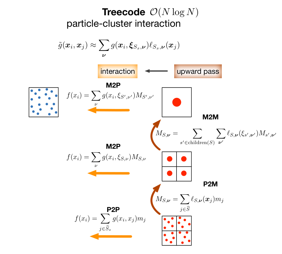
A schematic comparison of treecode [20] and FMM is illustrated in Figure 1. In the treecode (Figure 1(a)), we interpolate the source variable $\bm{x}_{j}$ of the kernel function so that we can cluster the source particles and build up the effective masses of each cluster. The force-field of each particle in the target cluster is evaluated by each independent traversal of the source cluster tree and by investigating the particle-cluster interaction. In the FMM (Figure 1(b)), we interpolate both target variable $\bm{x}_{i}$ and source variable $\bm{x}_{j}$ of the kernel function so that the target particles and source particles can be clustered and the corresponding effective force-fields and masses of each cluster can be built up. The force-field on a target particle is transferred from the effective force-fields of the clusters, which are computed by cluster-cluster interaction through the traversal of the target cluster tree and the source cluster tree simultaneously.

The pseudocodes for the algorithms are presented with the following global variables:

The algorithms described above are implemented as a solver in the Julia programming language [26]. The cluster tree constructed with Algorithm 5.2 is implemented using a pointer-based data structure.

To understand the performance of the proposed FMM, we first demonstrate a plot of elapsed time against the error for the simulations with different FMM parameters in Figure 2. In each simulation, $1.28\times 10^{6}$ particles are randomly uniformly distributed in the unit cube $[0,1]^{3}$ and each particle has the same momentum $\bm{p}=(0,0,p_{0})$ with $p_{0}=(\gamma^{2}-1)^{1/2}$ and $\gamma=50$. The measured error is the maximal relative error in the electrical and magnetic fields,

where $N$ is the number of particles in the system. The space-charge fields $\bm{f}^{t}_{i}$ and $\bm{f}^{b}_{i}$ experienced by the $i$-th particle are computed by FMM and a brute-force method ( Algorithm 5.10 with $S_{t}=S_{s}=S$ and $i\neq j$), respectively. We can observe that a smaller admissibility parameter $\eta$ (4.3) leads to higher accuracy (smaller error) but costs more elapsed time. This is because fewer M2Ls in the coarse level are performed and each non-admissible pair of clusters in the coarse level can result in many M2Ls in the finer level or P2Ps in the leaf level.

The usage of a higher interpolation degree $n$ leads to a result with higher accuracy and higher elapsed time because more macro particles are used in the calculation of M2L. In Figure 3, the elapsed time of FMM against the number of particles $N$ is presented. We can see that our FMM approaches the theoretical complexity $\mathcal{O}(N)$ as the number of particles $N$ becomes big enough (Figure 3(b)).

We also perform code profiling on our solver and demonstrate the cumulative elapsed time of the six FMM kernels in Figure 4. One can observe that the total elapsed time is mostly dominated by P2P and M2L; this indicates that the routines of these two kernels will be the focus when any further optimizations for the solver are considered. Besides, one can also observe a sudden jump in the value of the elapsed times for P2P and M2L at a specific number of particles $N$. To understand this phenomenon, we consider a case where the total particle number is equal to a transition value $N=N^{\kappa}_{t}:=2^{\kappa}N_{0}$ with $\kappa$ the depth of the cluster tree. If each leaf cluster interacts with at most a constant number of clusters via P2P, the total number of operation counts to perform P2P can be written as

When the number of particles $N$ slightly increases with $\delta N\to 0$ so that $N>N^{\kappa}_{t}$, the number of particles in each leaf cluster $N_{\text{f}}$ will slightly increase with $\delta N_{\text{f}}\to 0$ so that $N_{\text{f}}>N_{0}$. In this case, each leaf cluster will be subdivided into two clusters and the cluster tree will gain one more level $\kappa+1$. Therefore, the number of leaf clusters will increase from $2^{\kappa}$ to $2^{\kappa+1}$ and the value of $N_{\text{f}}$ reduces from $N_{0}$ to $N_{0}/2$. Thus, the total number of operation counts for P2P can be written as

References

- [1] H. Zhang, J. Portman, Z. Tao, P. Duxbury, C.-Y. Ruan, K. Makino, M. Berz, The Differential Algebra Based Multiple Level Fast Multipole Algorithm for 3D Space Charge Field Calculation and Photoemission Simulation, Microscopy and Microanalysis 21 (S4) (2015) 224–229. doi:10.1017/S1431927615013410.
- [2] H. Zhang, H. Huang, R. Li, J. Chen, L.-S. Luo, Fast multipole method using Cartesian tensor in beam dynamic simulation, AIP Conference Proceedings 1812 (1) (2017) 050001. doi:10.1063/1.4975862.
- [3] M. Langston, R. Lethin, P. Letourneau, M. Morse, J. Wei, MACH-B: Fast Multipole Method Approaches in Particle Accelerator Simulations for the Computational and Intensity Frontiers, in: Proceedings of the 12th International Particle Accelerator Conference, no. 12 in International Particle Accelerator Conference, JACoW Publishing, Geneva, Switzerland, 2021, pp. 4237–4240. doi:10.18429/JACoW-IPAC2021-THPAB227.
- [4] M. Gordon, S. Van Der Geer, J. Maxson, Y.-K. Kim, Point-to-point Coulomb effects in high brightness photoelectron beam lines for ultrafast electron diffraction, Physical Review Accelerators and Beams 24 (8) (2021) 084202. doi:10.1103/PhysRevAccelBeams.24.084202.
- [5] S. Schmid, H. De Gersem, M. Dohlus, E. Gjonaj, Simulating Space Charge Dominated Beam Dynamics Using FMM, in: Proceedings of 3rd North American Particle Accelerator Conference, 2019, p. WEPLE10. doi:10.18429/JACoW-NAPAC2019-WEPLE10.
- [6] J. M. Dawson, Particle simulation of plasmas, Reviews of Modern Physics 55 (1983) 403–447. doi:10.1103/RevModPhys.55.403.
- [7] C. K. Birdsall, A. B. Langdon, Plasma Physics via Computer Simulation, CRC press, 2018.
- [8] K. Flöttmann, S. Lidia, P. Piot, Recent improvements to the ASTRA particle tracking code, Tech. rep., Lawrence Berkeley National Lab (LBNL), USA (2003).
- [9] J. Qiang, S. Lidia, R. D. Ryne, C. Limborg-Deprey, Three-dimensional quasistatic model for high brightness beam dynamics simulation, Phys. Rev. ST Accel. Beams 9 (2006) 044204. doi:10.1103/PhysRevSTAB.9.044204.
- [10] J. Qiang, Symplectic particle-in-cell model for space-charge beam dynamics simulation, Phys. Rev. Accel. Beams 21 (2018) 054201. doi:10.1103/PhysRevAccelBeams.21.054201.
- [11] F. W. Jones, A hybrid fast-multipole technique for space-charge tracking with halos, AIP Conference Proceedings 448 (1) (1998) 359–370. doi:10.1063/1.56759.
- [12] S. A. Schmid, H. D. Gersem, E. Gjonaj, REPTIL - A Relativistic 3D Space Charge Particle Tracking Code Based on the Fast Multipole Method, unpublished (01 2019).
- [13] J. Qiang, Symplectic multiparticle tracking model for self-consistent space-charge simulation, Physical Review Accelerators and Beams 20 (2017) 014203. doi:10.1103/PhysRevAccelBeams.20.014203.
- [14] S. Schmid, H. D. Gersem, E. Gjonaj, Energy-Binning Fast Multipole Method for Electron Injector Simulations, in: Proceedings of the 12th International Particle Accelerator Conference, no. 12 in International Particle Accelerator Conference, JACoW Publishing, Geneva, Switzerland, 2021, pp. 4244–4246. doi:10.18429/JACoW-IPAC2021-THPAB229.
- [15] G. Fubiani, J. Qiang, E. Esarey, W. P. Leemans, G. Dugan, Space charge modeling of dense electron beams with large energy spreads, Phys. Rev. ST Accel. Beams 9 (2006) 064402. doi:10.1103/PhysRevSTAB.9.064402.
- [16] Y.-K. Kan, F. X. Kärtner, S. Le Borne, J.-P. M. Zemke, Relativistic space-charge field calculation by interpolation-based treecode, Computer Physics Communications 286 (2023) 108668. doi:10.1016/j.cpc.2023.108668.
- [17] L. Wilson, N. Vaughn, R. Krasny, A GPU-accelerated fast multipole method based on barycentric Lagrange interpolation and dual tree traversal, Computer Physics Communications 265 (2021) 108017. doi:10.1016/j.cpc.2021.108017.
- [18] S. Wienke, P. Springer, C. Terboven, D. an Mey, Openacc — first experiences with real-world applications, in: C. Kaklamanis, T. Papatheodorou, P. G. Spirakis (Eds.), Euro-Par 2012 Parallel Processing, Springer Berlin Heidelberg, Berlin, Heidelberg, 2012, pp. 859–870.
- [19] W. Fong, E. Darve, The black-box fast multipole method, Journal of Computational Physics 228 (23) (2009) 8712–8725. doi:10.1016/j.jcp.2009.08.031.
- [20] L. Wang, R. Krasny, S. Tlupova, A kernel-independent treecode based on barycentric Lagrange interpolation, Communications in Computational Physics 28 (4) (2020) 1415–1436. doi:10.4208/cicp.OA-2019-0177.
- [21] L. Wilson, Development and Application of Numerical Methods in Biomolecular Solvation, Ph.D. thesis, University of Michigan (2021). doi:10.7302/1547.
- [22] S. Börm, Efficient numerical methods for non-local operators: -matrix compression, algorithms and analysis, Vol. 14 of EMS Tracts in Mathematics, European Mathematical Society (EMS), Zürich, 2010. doi:10.4171/091.
- [23] W. Hackbusch, Hierarchical Matrices: Algorithms and Analysis, Vol. 49, Springer, 2015. doi:10.1007/978-3-662-47324-5.
- [24] A. W. Appel, An efficient program for many-body simulation, SIAM Journal on Scientific and Statistical Computing 6 (1) (1985) 85–103. doi:10.1137/0906008.
- [25] W. Dehnen, A Hierarchical O(N) Force Calculation Algorithm, Journal of Computational Physics 179 (1) (2002) 27–42. doi:10.1006/jcph.2002.7026.
- [26] J. Bezanson, A. Edelman, S. Karpinski, V. B. Shah, Julia: A Fresh Approach to Numerical Computing, SIAM Review 59 (1) (2017) 65–98. doi:10.1137/141000671.
- [27] J. Liu, M. Robson, T. Quinn, M. Kulkarni, Efficient GPU Tree Walks for Effective Distributed N-Body Simulations, in: Proceedings of the ACM International Conference on Supercomputing, ICS ’19, Association for Computing Machinery, New York, NY, USA, 2019, p. 24–34. doi:10.1145/3330345.3330348.
- [28] M. Burtscher, K. Pingali, Chapter 6 - An Efficient CUDA Implementation of the Tree-Based Barnes Hut n-Body Algorithm, in: W. mei W. Hwu (Ed.), GPU Computing Gems Emerald Edition, Applications of GPU Computing Series, Morgan Kaufmann, Boston, 2011, pp. 75–92. doi:10.1016/B978-0-12-384988-5.00006-1.
- [29] Leighton Wilson, private communication (2022).
- [30]
L. Wilson, N. Vaughn, BaryTree
(2021).
URL https://github.com/Treecodes/BaryTree - [31] J. Cheng, M. Grossman, T. McKercher, Professional CUDA C Programming, John Wiley & Sons, 2014.
- [32]
A. Ferris, other contributors,
StaticArrays (2016).
URL https://github.com/JuliaArrays/StaticArrays.jl - [33]
Julia Computing, other contributors,
CUDA.jl (2016).
URL https://github.com/JuliaArrays/StaticArrays.jl - [34] T. Besard, C. Foket, B. D. Sutter, Effective Extensible Programming: Unleashing Julia on GPUs, IEEE Transactions on Parallel and Distributed Systems 30 (4) (2019) 827–841. doi:10.1109/tpds.2018.2872064.
- [35] T. H. Cormen, C. E. Leiserson, R. L. Rivest, C. Stein, Introduction to algorithms, 4th Edition, MIT press, 2022.