Differentially Private Diffusion Auction: The Single-unit Case

Fengjuan Jia Affiliation: School of Computer Science and Engineering, University of Electronic Science and Technology of China Mengxiao Zhang Affiliation: School of Computer Science and Engineering, University of Electronic Science and Technology of China Jiamou Liu Affiliation: School of Computer Science, The University of Auckland Bakh Khoussainov Affiliation: School of Computer Science and Engineering, University of Electronic Science and Technology of China

Abstract

Diffusion auction refers to an emerging paradigm of online marketplace where an auctioneer utilises a social network to attract potential buyers. Diffusion auction poses significant privacy risks. From the auction outcome, it is possible to infer hidden, and potentially sensitive, preferences of buyers. To mitigate such risks, we initiate the study of differential privacy (DP) in diffusion auction mechanisms. DP is a well-established notion of privacy that protects a system against inference attacks. Achieving DP in diffusion auctions is non-trivial as the well-designed auction rules are required to incentivise the buyers to truthfully report their neighbourhood. We study the single-unit case and design two differentially private diffusion mechanisms (DPDMs): recursive DPDM and layered DPDM. We prove that these mechanisms guarantee differential privacy, incentive compatibility and individual rationality for both valuations and neighbourhood. We then empirically compare their performance on real and synthetic datasets.

1 Introduction

New technological shift in AI and data science has given rise to an imminent need to address data privacy issues in online platforms. Indeed, a Gartner survey shows that $41\%$ of the surveyed organisations have experienced a privacy breach or security incident¹¹ 1 https://blogs.gartner.com/avivah-litan/2022/08/05/ai-models-under-attack-conventional-controls-are-not-enough/. Data privacy issues have been especially serious and impactful around the use of social commerce platforms such as Instagram and Facebook. As users of such a platform find, browse and buy products through the social network, they are also exposed to a significant risk of privacy leakage. A recent PCI Pal survey shows that fewer than $7\%$ of users are confident about their data security on social commerce sites²² 2 https://www.pcipal.com/knowledge-centre/resource/fewer-than-10-of-people-are-confident-about-their-data-security-on-social-media-according-to-survey-from-pci-pal/. Thus designing new tools to facilitate safe and private use of social commerce platforms is of crucial importance.

Auction is important in facilitating online commerce. Auctions have been applied in many contexts, e.g., radio spectrum, sponsored search ads, virtual resource allocation. In an auction, buyers submit their (private) valuations in bids to the auctioneer. The bids often imply buyers’ preferences and confidential business strategies, and competitors may exploit them to gain an advantage. Hence, there is a need to protect the privacy of bid information. The privacy issues in auctions have recently been studied in [McSherry and Talwar 2007, Jian et al. 2018, Zhu et al. 2014, Ni et al. 2021]. To mitigate privacy risks, these studies employ the well-established notion of differential privacy (DP) [Dwork et al. 2006]. Here, DP is used to protect individual’s bid information when the auction outcome is published. To achieve DP on bids, the work of McSherry and Talwar 2007 proposed exponential mechanism. The mechanism randomises auction results so that a change in a buyer’s bid does not significantly affect the auction outcome. In this way, the mechanism prevents the bid from being inferred from the auction outcome. This mechanism has so far been a predominant method to protect privacy in auctions.

Diffusion auction is an emerging form of auction. In this setting, a seller is able to harness the power of social network to diffuse auction information, inviting friends, friends-of-friends, etc., to join the auction, thereby attracting a large number of potential buyers. This differs from a standard auction (without social network) where the participants are fixed beforehand. Thus, diffusion auction are especially suitable for facilitating online social commerce platforms where the social network plays a prominent role. A challenge in diffusion auctions lies in resolving the conflict between the seller who wants to attract more participants for better revenue and the buyers who are reluctant to invite their friends to avoid competition. Thus there is a need to extend incentive compatibility (IC) for hidden valuations in classical auctions, to diffusion IC for hidden valuation as well as social ties. Numerous studies, e.g., [Li et al. 2017, Li et al. 2019, Zhang et al. 2020b, Zhang et al. 2020a], have proposed mechanisms for diffusion auction that achieve diffusion IC.

Diffusion auctions are prone to all aforementioned privacy risks for auctions in general. However, no study has focused on the privacy issues for diffusion auctions. Here we close this gap by investigating the following question:

How do we design a differentially private diffusion mechanism (DPDM) that guarantees desirable properties and preserves valuation privacy?

Answering this question is not a trivial task. As mentioned above, the exponential mechanism is the main approach to ensure DP for auctions. An exponential mechanism firstly creates a probability distribution over all possible auction results such that more preferable result is associated with a higher probability, and then outputs an auction result according to the distribution. However, this mechanism can not be directly extended to diffusion auctions as it fails to ensure diffusion IC property. For instance, run the exponential mechanism to the scenario in Figure 1 (See Example 4.1 for a detailed implementation). Assume that all buyers except buyer $b$ reveal their neighbours truthfully. From $b$ ’s perspective, revealing her neighbour $f$ means getting a lower probability of winning the auction, as the exponential mechanism would distribute the winning probabilities over $7$ buyers instead of $5$ . Therefore, the buyers are not incentivised to diffuse auction information to their friends.

Refer to caption — Figure 1: A social network with a seller $s$ and seven buyers. The number beside each node is the valuations of the buyer. The seller $s$ has an item to sell, and initially knows only $a,b,c$ . The mechanism will construct a probability distribution over potential buyers which determines how likely a buyer is to win the item.

Contribution. In this paper, we design a DPDM for the single-unit auction case where a single seller sells one indivisible item to multiple potential buyers. The seller and the buyers are assumed to be nodes in a social network with their connections represented as edges. The seller initially only has access to her direct neighbours, and must incentivise the buyers to truthfully report both their valuations of the item, and their neighbourhood. At the same time, the DPDM should ensure the DP property for buyers’ bids. We design two DPDMs: recursive DPDM and layered DPDM. The idea for these two mechanisms is market division that partitions the buyers into sub-markets. The mechanism then associates a probability with each sub-market. To ensure diffusion IC, the probability should be monotonic on the size of the sub-markets:

•

The recursive DPDM maps the network into a tree that captures information flow among buyers. Then it recursively divides the market such that each sub-tree is a sub-market and its probability is non-decreasing on the size of the sub-tree.
•

The layered DPDM also relies on the tree above, except the market is not partitioned by sub-trees, but rather by buyers’ distances from the seller. In this way, each layer is a sub-market and its probability is fixed.

These two mechanisms are proven to meet all the desirable properties. The layered DPDM has a lower bound on expected social welfare. The recursive DPDM achieves a better social welfare empirically. We demonstrate this using a series of experiments that simulate diffusion auctions over three real-world social network datasets. Our experiments reveal that in most cases, the recursive DPDM reaches comparable social welfare as the theoretical upper bound. We now highlight our contributions:

1.

We expand diffusion mechanisms adding the DP condition. This builds a bridge between diffusion auctions and privacy preservation. See Section 3.2.
2.

Using the idea of market division, we design recursive DPDM (Section 4) and layered DPDM (Section 5). These mechanisms are IC and differentially private.
3.

We empirically evaluate our two mechnaisms on real-world network datasets. See Section 6.

2 Related work

Differentially private mechanism.

Differential privacy (DP) is proposed to protect individual data from inference attacks on an aggregate query over a database [Dwork et al. 2006]. The notion has since been extended to various domain such as statistical data inference [Dwork 2008], decision trees [Fletcher and Islam 2019], and unstructured data [Zhao and Chen 2022]. McSherry and Talwar 2007 extend DP to auctions and propose exponential mechanism. This mechanism ensures a weaker version of IC, namely approximate IC, which ensures that any user can only gain a bounded extra utility from misreporting. This solution concept is adopted in subsequent studies [Zhu et al. 2014] and [Diana et al. 2020] on multi-item auctions and one-shot double auctions. As approximate IC allows bidders to have non-zero incentives to lie, these methods would not meet the requirements in our problem.

Many works design DP auctions that ensure traditional version of IC [Huang and Kannan 2012, Xiao 2013, Zhu and Shin 2015, Jian et al. 2018]. Specifically, Huang and Kannan 2012, Xiao 2013 propose general methods to transform a classical IC mechanism to a privacy preserving counterpart that is still IC. The method of [Xiao 2013] works only when the valuation space is small and can not be applied to general problems, including ours. In contrast, the transformation method in [Huang and Kannan 2012] can be applied to more general problems. The transformed mechanism can be seen as a generalisation of Vickrey-Clarke-Groves (VCG) mechanism [Groves 1973], which is paired with a carefully designed payment rule. However, when the mechanism is applied to multi-item auctions, it is approximately IC rather than IC. Later, Zhu and Shin 2015 and Xu et al. 2017, Jian et al. 2018 propose mechanisms that combine the exponential mechanism with the payment rule in [Archer and Tardos 2001], applying to combinatorial auctions and reverse auctions, respectively.

No mechanism above can be applied to our problem of designing DPDM because they fail to ensure diffusion IC. We next introduce existing diffusion auction mechanisms.

Diffusion auction.

Diffusion auction is an emerging topic in mechanism design. Li et al. 2017 are the first to investigate diffusion auction and propose information diffusion mechanism (IDM), a mechanism for single-unit auction in a social network. The basic idea is to give monetary reward to buyers who are critical to diffusion, and it ensures diffusion IC. Following this idea, Li et al. 2019, Zhang et al. 2020b, Zhang et al. 2020a further study single-unit diffusion auction from different aspects. Later, Zhao et al. 2018, Kawasaki et al. 2020 extend single-unit diffusion auctions to multiple-unit cases and propose generalised IDM (GIDM) and DNA-MU, resp. However, all of these mechanisms are deterministic and suffer from privacy leakage risks.

3 Problem formulation

3.1 Preliminaries

Consider the following setup: There is a seller, denoted by $s$ , and $n$ buyers, denoted by $N=\{1,2,3,...,n\}$ . Seller $s$ has a single indivisible item to sell. Each buyer $i\in N$ is willing to buy the item and attaches a valuation $v_{i}$ to the item. Valuation $v_{i}$ is the maximum amount of money that $i$ is willing to pay. This value is private to the seller.

The seller and the buyers form a social network, represented by a graph $G=(V,E)$ , where $V=N\cup\{s\}$ is the vertex set and $E\subseteq V^{2}$ is the edge set. Each node $i\in V$ has a neighbour set, denoted by $r_{i}\coloneqq\{j\in V\mid(i,j)\in E\}$ . We assume that only the seller’s neighbours know the auction information initially. The seller would like to attract more buyers to participate in the auction and spread the auction information. Each buyer is able to deliver the auction information to her neighbours. The set $r_{i}$ is also a private information of buyer $i$ .

Each buyer $i\in N$ , once informed with the auction, can participate in the auction. Also, for each buyer a pair consisting of her valuation and neighbour set is called the profile of the buyer. We use $\theta_{i}\coloneqq(v_{i},r_{i})$ to denote this profile. The profile is known to the buyer and it is hidden to anyone else. Let $\Theta$ denote the set of all possible profiles. Also, we let $\theta\coloneqq(\theta_{1},\ldots,\theta_{n})$ be the global profile of all buyers and $\theta_{-i}\coloneqq(\theta_{1},\ldots\theta_{i-1},\theta_{i+1},\ldots\theta_{n})$ be the global profile of all buyers except for $i$ . In the auction, each buyer is asked to report her profile $\theta_{i}^{\prime}=(v_{i}^{\prime},r_{i}^{\prime})$ , which is not necessarily the true one. We define $\theta^{\prime}\in\Theta^{n}$ as the reported global profile of all buyers. Given $\theta^{\prime}$ , we construct a directed graph $G_{\theta^{\prime}}=(V_{\theta^{\prime}},E_{\theta^{\prime}})$ : add a directed edge $(i,j)$ if $j$ is reported by $i$ as a neighbour. We call such graph profile digraph.

Diffusion auction has two forms of information asymmetry: (1) Valuation asymmetry. The buyers’ true valuations are private information and hidden from the seller. Thus buyers have an advantage over the seller as they can misreport their valuations. The auction should prevent misreporting of valuation through appropriate allocation and pricing strategies. (2) Neighbourhood asymmetry. By Bulow-Klemperer theorem, the revenue of an auction increases as the number of buyers grows [Bulow and Klemperer 1996]. However, as buyers’ neighbours on the social network are hidden, the seller would hope the buyers to diffuse the auction information to their neighbours to allow more participants to join. However, being rational, the buyers are not necessarily willing to disseminate the auction information as this may hinder their own chance of winning. Here, we follow the standard convention and assume that the reported neighbour set $r_{i}^{\prime}$ is a subset of $r_{i}$ .

Diffusion auction mechanisms are designed to address these two challenges. Now we give the definition of a mechanism. A mechanism, denoted by $M$ , takes the reported global profile $\theta^{\prime}$ of all buyers as input, and determines who is allocated the item and how much to pay.

Definition 3.1.

A mechanism $M$ consists of two functions $(\pi(\cdot),$ $p(\cdot))$ , where $\pi\colon\Theta^{n}\to\{0,1\}^{n}$ is an allocation function and $p\colon\Theta^{n}\to\mathbb{R}^{n}$ is a payment function.

The allocation function determines whether the buyers get the item while the payment function determines the amount of money that the buyers need to pay. Given a reported global profile $\theta^{\prime}$ of all buyers, we write the allocation result $\pi(\theta^{\prime})$ as $(\pi_{1}(\theta^{\prime}),\ldots,$ $\pi_{n}(\theta^{\prime}))$ and the payment result $p(\theta^{\prime})$ as $(p_{1}(\theta^{\prime}),\ldots,p_{n}(\theta^{\prime}))$ , where $\pi_{i}(\theta^{\prime})$ and $p_{i}(\theta^{\prime})$ is buyer $i$ ’s allocation and payment. The utility of buyer $i$ with profile $\theta_{i}=(v_{i},r_{i})$ is $u_{i}(\theta^{\prime})=v_{i}\pi_{i}(\theta^{\prime})-p_{i}(\theta^{\prime})$ when reported global profile is $\theta^{\prime}$ . The social welfare of mechanism $M$ on $\theta^{\prime}$ , denoted by $sw_{M}(\theta^{\prime})$ , is defined as the sum of the seller and the buyers’ utility, i.e., $sw_{M}(\theta^{\prime})=\sum_{i\in V}u_{i}(\theta^{\prime})$ . We aim to maximise the social welfare.

3.2 Privacy-aware diffusion auction

In addition to Challenges (1) and (2) above, we consider a third challenge in diffusion auction when the buyers are privacy-aware. (3) Valuation privacy. Once the auction result is annouced, an attacker with certain background information may infer the bid information from the published auction result. This is known as the inference attack [Li et al. 2017]. This disadvantages the buyer(s) whose private valuation is diclosed. Therefore, the buyers require the guarantees that their private valuations are protected.

To achieve privacy preservation, we apply a randomised mechanism $M$ to implement an auction on the reported global profile.

Definition 3.2.

A randomised mechanism $M$ is one that, given a global profile $\theta$ , outputs a pair $(\pi,p)$ such that $\pi$ is a randomised allocation function and $p$ is a randomised payment function.

Given a global profile $\theta$ , the randomised mechanism $M$ outputs $\pi(\theta)$ and $p(\theta)$ such that $\pi(\theta)$ is a random variable with possible values $\{0,1\}^{n}$ and $p(\theta)$ is a random variable with possible values $(\mathbb{R}^{+})^{n}$ . We use the concept of differential privacy to define the privacy protection of a mechanism. Basically, differential privacy requires that the distributions over the outcomes are nearly identical when the global profiles are nearly identical. The privacy protection level is measured by a privacy parameter $\epsilon\in\mathbb{R}^{+}$ .

Definition 3.3.

A randomised mechanism $M$ is $\epsilon$ -differential privacy ( $\epsilon$ -DP) if for any two global profiles $\theta,\theta^{\prime}\in\Theta^{n}$ that differ on a single buyer’s valuation, and for any possible outcome $o\in O$ ,

\mathrm{Pr}[M(\theta)=o]\leq\exp(\epsilon)\mathrm{Pr}[M(\theta^{\prime})=o]

(1)

Eqn. (1) shows if any buyer $i$ changes her reported profile from $\theta_{i}=(v_{i},r_{i})$ to $\theta_{i}^{\prime}=(v_{i}^{\prime},r_{i})$ , the auction outcome does not change too much. Therefore, no one could infer the valuation of any buyer from the randomised outcome.

Exponential mechanism [McSherry and Talwar 2007] is an existing mechanism that ensures $\epsilon$ -DP for valuation privacy. Given a global profile, an exponential mechanism creates a distribution over all possible auction outcomes, and outputs an outcome according to the distribution. Intuitively, the higher a reported valuation is, the more likely the corresponding buyer is selected as a winner. Specially, given a global profile $\theta$ , define a score function $\sigma\colon\Theta^{n}\times O\to\mathbb{R}$ that assigns a real valued score to each pair $(\theta,o)$ from $\Theta^{n}\times O$ . The more preferable an outcome is, the higher the score of the outcome is. An exponential mechanism $M(\theta)$ outputs a result $o^{*}\in O$ with probability

\frac{\exp(\epsilon\sigma(\theta,o^{*}))}{\sum_{o\in O}\exp(\epsilon\sigma(\theta,o))}

In our problem, a result corresponds to that a certain buyer $i$ wins, and we use $o_{i}$ to denote this result.

In randomised mechanisms, we assume that the buyers are risk-neutral and care about their utilities in expectation. We use $\mathbf{E}_{M}[u_{i}(\cdot)]$ to denote $i$ ’s expected utility in $M$ and redefine the standard IC and IR properties by expected utility.

Definition 3.4.

Let $M$ be a randomised mechanism,

•

The mechanism $M$ is IC if for all $i\in N$ , all $\theta_{i},\theta_{i}^{\prime}\in\Theta$ and for all $\theta_{-i}^{\prime},\theta_{-i}^{\prime\prime}\in\Theta^{n-1}$ , we have the following, $\mathbf{E}_{M}[u_{i}((\theta_{i},\theta_{-i}^{\prime}))]\geq\mathbf{E}_{M}[u_{i}((\theta_{i}^{\prime},\theta_{-i}^{\prime\prime}))].$
•

The mechanism $M$ is IR if for all $i\in N$ and all $\theta_{-i}^{\prime}\in\Theta^{n-1}$ , we have $\mathbf{E}_{M}[u_{i}((\theta_{i},\theta_{-i}^{\prime}))]\geq 0.$

The IR and IC properties ensure that buyers are willing to participate in the auction and to reveal their true valuations and neighbours, as they are rational and doing so leads to the best expected utilities. Hence, information asymmetry issues can be addressed.

The social welfare of $M$ is also in expectation, i.e.,

\mathbf{E}_{M}[sw_{M}(\theta)]=\sum_{i\in V}\mathbf{E}_{M}[u_{i}(\theta)].

We aim to design a randomised mechanism that is IC, IR, $\epsilon$ -DP (for reasonable $\epsilon$ ) while maximising social welfare.

4 Recursive DPDM

Preserving valuation privacy in diffusion auctions is not a trivial task. On one hand, existing diffusion auctions, including IDM [Li et al. 2017], CMD [Li et al. 2019], and FDM [Zhang et al. 2020b], are deterministic, and thus fail to preserve privacy. On the other hand, existing differential private mechanisms, including exponential mechanism, fail to incentivise truthful report of neighbours, which is illustrated in Example 4.1.

Example 4.1.

We apply exponential mechanism paired with score function $\sigma(\theta,o_{i})=v^{\prime}_{i}$ to the scenario in Figure 1. That is, the score of the result that $i$ wins is $i$ ’s reported valuation $v_{i}^{\prime}$ . We assume that the buyers truthfully report their valuations. Then buyer $i$ wins with probability $\exp(\epsilon v_{i})/\sum_{\kappa\in N}\exp(\epsilon v_{\kappa})$ . Now if buyer $b$ reports her neighbour $f$ , $b$ wins with probability $\exp(8\epsilon)/\sum_{\kappa\in N}\exp(\epsilon v_{\kappa})$ , whereas she wins with probability $\exp(8\epsilon)/\sum_{\kappa\in N\setminus\{f,j\}}\exp(\epsilon v_{\kappa})$ had she chose not to report $f$ . In the latter case, the winning probability is even higher, and thus $b$ has incentive to hide her neighbours.

To incentivise buyers to diffuse auction information, we need to ensure each buyer’s utility of reporting her neighbours should be no less than that of non-reporting. We now propose recursive DPDM ${\mathrm{REC}}$ to achieve this condition. The basic idea is “market division”, i.e., treat the social network as a market, partition the market into multiple sub-markets and assign each sub-market a probability with which buyers in this sub-market win, as shown in Eqn. (2). In this case, each buyer would report as many neighbours as possible in order to maximise the probability of the sub-market she belongs to. Then the buyers in a sub-market share the probability of the sub-market in such a way that the winning probability of any buyer is independent from her children, as shown in Eqn. (3). Therefore, the buyers have no competition with their children and have no incentive to misreport them.

We now describe ${\mathrm{REC}}$ in detail: Fix a score function $\sigma(\cdot)$ that is non-decreasing in reported valuation $v_{i}^{\prime}$ . Given a reported global profile $\theta^{\prime}$ , a privacy parameter $\epsilon$ and the score function $\sigma(\cdot)$ as input, ${\mathrm{REC}}$ works as follows:

(1) Construction of diffusion critical tree. Given a profile digraph $G_{\theta^{\prime}}$ , ${\mathrm{REC}}$ first constructs a diffusion critical tree, denoted by $T_{\theta^{\prime}}$ . When the context is clear, we write the tree as $T$ . The idea of diffusion critical tree is originally introduced by [Zhao et al. 2018]. For any buyers $i,j\in V_{\theta^{\prime}}$ , we say that $i$ is $\theta^{\prime}$ -critical to $j$ , denoted by $i\preceq_{\theta^{\prime}}j$ , if all paths from $s$ to $j$ in $G_{\theta^{\prime}}$ go through $i$ . A diffusion critical tree is a rooted tree, where the root is seller $s$ and the nodes $V_{\theta^{\prime}}$ are the buyers who are connected to $s$ , and for each $j\in V_{\theta^{\prime}}$ , her parent is the node $i\preceq_{\theta^{\prime}}j$ who has the closest distance to $j$ . When there are more than one parents, only one node is randomly selected as the parent. The depth of buyer $i$ , denoted by $d_{i}$ , is the distance from $s$ to $i$ .

(2) Assignment of winning probabilities. This step determines the probabilities that buyers win the item. This is a recursive process. This process starts with the constructed $T$ rooted by $s$ . Given a (sub-)tree rooted by $i\in V$ , ${\mathrm{REC}}$ assigns a probability to each sub-tree rooted by $j\in r_{i}$ , and a winning probability to each $j\in r_{i}$ . This operation is repeated for $j$ ’s children, children of $j$ ’s children and so on until there is no more children.

(a) Assignment of probabilities to sub-trees. Let $T[i]$ denote the sub-tree rooted by $i$ . $T[i]$ consists of node $i$ and all of $i$ ’s descendants. Let $T(i)$ denote $T[i]$ with $i$ removed, i.e., $T(i)\coloneqq T[i]\setminus\{i\}$ . Given a sub-tree $T[i]$ , ${\mathrm{REC}}$ divides the market in $T[i]$ to $|r_{i}|+1$ sub-markets, one for $i$ and each of the other for a sub-tree $T[j]$ , where $j\in r_{i}$ . Then ${\mathrm{REC}}$ assigns a probability $\mathrm{Pr}_{i}^{\theta^{\prime}}(\theta_{i}^{\prime})$ to $i$ with $\theta_{i}^{\prime}$ and $\mathrm{Pr}^{\theta^{\prime}}_{T[j]}$ to each $T[j]$ , where $j\in r_{i}$ . When the context is clear, we write $\mathrm{Pr}_{i}$ and $\mathrm{Pr}_{T[j]}$ for $\mathrm{Pr}_{i}^{\theta^{\prime}}(\theta_{i}^{\prime})$ and $\mathrm{Pr}^{\theta^{\prime}}_{T[j]}$ , respectively. We define $\mathrm{Pr}_{i}$ later in Step (2).b. For notational convenience, given a set of nodes $S\subseteq T$ , we let $\mathrm{Exp}(S)$ be the sum

\mathrm{Exp}(S)=\sum_{\kappa\in S}\exp(\epsilon\sigma(\theta^{\prime},o_{\kappa})).

Now we define $\mathrm{Pr}_{T[j]}$ for each $j\in r_{i}$ as

\mathrm{Pr}_{T[j]}=\left(\mathrm{Pr}_{T[i]}-\mathrm{Pr}_{i}\right)\times\frac{\mathrm{Exp}(T[j])}{\mathrm{Exp}(T(i))}

(2)

(b) Assignment of winning probabilities to buyers within a sub-market. In a sub-tree $T[i]$ , ${\mathrm{REC}}$ assigns the winning probability $\mathrm{Pr}_{j}$ to each $j\in r_{i}$ as

\mathrm{Pr}_{j}=\left(\mathrm{Pr}_{T[i]}-\mathrm{Pr}_{i}\right)\times\frac{\mathrm{Exp}(j)}{\mathrm{Exp}(T(i)\setminus T(j))}

(3)

At the very beginning, ${\mathrm{REC}}$ starts with the tree $T$ rooted by $s$ . We label $s$ as node $0$ and set $\mathrm{Pr}_{T[0]}=1$ and $\mathrm{Pr}_{0}=0$ . ${\mathrm{REC}}$ ends with the leaves. For a sub-tree $T[i]$ where each $j\in r_{i}$ are leaves, ${\mathrm{REC}}$ assigns the winning probability to each $j$ as $\mathrm{Pr}_{j}=\left(\mathrm{Pr}_{T[i]}-\mathrm{Pr}_{i}\right)\times\frac{\mathrm{Exp}(j)}{\mathrm{Exp}(T(i))}$ .

(3) Allocation and payment. Randomly select a buyer $w$ as a winner according to the constructed distribution in Step (2). Set $w$ ’s allocation $\pi_{w}=1$ , and payment as

p_{w}=v_{w}^{\prime}-\int_{0}^{v_{w}^{\prime}}\mathrm{Pr}_{w}((x,r_{w}^{\prime}))dx/\mathrm{Pr}_{w}(\theta_{w}^{\prime})

(4)

We present the details of ${\mathrm{REC}}$ in Algorithm 1 and give a running example of Step (2) in Example 4.2.

Algorithm 1 Recursive DPDM

{\mathrm{REC}}

1: Reported global profile

\theta^{\prime}

, privacy parameter

\epsilon

and score function

\sigma

2: Allocation result

\pi(\theta^{\prime})

and payment result

p(\theta^{\prime})

3: Initialise

\pi(\theta^{\prime})=\textbf{0},p(\theta^{\prime})=\textbf{0}

4: Construct a profile digraph

G_{\theta^{\prime}}=(V_{\theta^{\prime}},E_{\theta^{\prime}})

5: Construct a critical diffusion tree

T_{\theta^{\prime}}

6: Run GetPro(

T_{\theta^{\prime}}[0],1,0

)

7: Randomly select a buyer

w

with the distribution

8: Set

\pi_{w}=1

and

p_{w}

by Equation (4)

Algorithm 2 GetPro

1: (Sub-)Tree

T[i]

, probabilities

\mathrm{Pr}_{T[i]}

and

\mathrm{Pr}_{i}

2: Probabilities

\mathrm{Pr}_{T[j]}

and

\mathrm{Pr}_{j}

j\in r_{i}

3: for

j\in r_{i}

4: Calculate

\mathrm{Pr}_{T[j]}

of sub-tree

T[j]

by Equation (2)

5: Calculate

\mathrm{Pr}_{j}

of buyer

j

by Equation (3)

6: Run GetPro(

T[j],\mathrm{Pr}_{T[j]},\mathrm{Pr}_{j}

)

7: end for

Example 4.2.

We apply ${\mathrm{REC}}$ paired with score function $\sigma(\theta,o_{i})=v^{\prime}_{i}$ to the scenario in Fig. 1. Firstly, $\mathrm{Pr}[T]=1$ and $\mathrm{Pr}_{s}=0$ . Next we calculate the probabilities of $s$ ’s children. The probability for $T[a]$ is $\mathrm{Pr}_{T[a]}=(\exp(10\epsilon)+\exp(9\epsilon)+\exp(12\epsilon))/{\mathrm{Exp}(T)}$ . Buyer $a$ wins with probability $\mathrm{Pr}_{a}(10)=\exp(10\epsilon)/(\mathrm{Exp}(T)-(\exp(9\epsilon)+\exp(12\epsilon)))$ . Similarly, we can get the probabilities for $T[b],T[c]$ and $b,c$ . Consider buyer $d$ . $d$ wins with probability $\mathrm{Pr}_{d}(9)=(\mathrm{Pr}(T[a])-\mathrm{Pr}_{a})\times\exp(9\epsilon)/(\exp(9\epsilon)+\exp(12\epsilon))$ . Similarly, we can also get the probabilities for $e,f,g$ .

Next we show that recursive DPDM satisfies IC, IR and DP. The next classical result is important for IC.

Theorem 4.3 ([Archer and Tardos 2001]).

Let $\mathrm{Pr}_{i}(v_{i}^{\prime})$ be the probability that $i$ wins when she reports $v_{i}^{\prime}$ . A mechanism $M=(\pi,p)$ is incentive compatible in terms of valuations if and only if, for any $i\in N$ ,

1.

$\mathrm{Pr}_{i}(v_{i}^{\prime})$ is monotonically non-decreasing in $v_{i}^{\prime}$ ;
2.

$\mathbf{E}[p_{i}]=v_{i}\mathrm{Pr}_{i}(v_{i}^{\prime})-\int_{0}^{v_{i}^{\prime}}\mathrm{Pr}_{i}(x)dx$

Lemma 4.4.

Recursive DPDM ${\mathrm{REC}}$ is incentive compatible in terms of both valuations and neighbours.

Proof.

We first show ${\mathrm{REC}}$ is IC in terms of valuations. By Equation (2), the probability for any sub-tree $T[i]$ is proportional to the score, which is non-decreasing in $v_{i}^{\prime}$ . Hence, $\mathrm{Pr}_{T[i]}$ in non-decreasing in $v_{i}^{\prime}$ . Similarly, by Equation (3), given a sub-tree $T[i]$ , the winning probability $\mathrm{Pr}_{i}$ is non-decreasing in $v_{i}^{\prime}$ , which meets the condition (1) in Thm. 4.3. Also, by Equation (4), the expected payment

\mathbf{E}[p_{i}]=p_{i}\times\mathrm{Pr}_{i}=v_{i}^{\prime}\mathrm{Pr}_{i}(\theta_{i}^{\prime})-\int_{0}^{v_{i}^{\prime}}\mathrm{Pr}_{i}((x,r_{i}^{\prime}))dx,

which meets the condition (2) in Theorem 4.3 when $r_{i}^{\prime}$ is fixed. Therefore, ${\mathrm{REC}}$ is IC in terms of valuations.

Next we show ${\mathrm{REC}}$ is IC in terms of neighbours. By the definitions of expected utility and payment function (4), we know that $i$ ’s expected utility is only determined by the winning probability $\mathrm{Pr}_{i}$ . Let $a^{\ell}$ be an ancestor of $i$ with distance $\ell$ . When $i$ reports truthfully as $\theta_{i}$ and the reported global profile is $\theta^{\prime}_{-i}$ , then $i$ ’s winning probability is

$\displaystyle\mathrm{Pr}_{i}=$	$\displaystyle\frac{\mathrm{Exp}(i)}{\mathrm{Exp}(T(a^{1})\setminus T(i))}\times(\mathrm{Pr}_{T[a^{1}]}-\mathrm{Pr}_{a^{1}})$	(5)
$\displaystyle=$	$\displaystyle\frac{\mathrm{Exp}(i)}{\mathrm{Exp}(T(a^{1})\setminus T(i))}\times\left(\mathrm{Pr}_{T[a^{2}]}-\mathrm{Pr}_{a^{2}}\right)$
	$\displaystyle\text{\qquad}\times\left(\frac{\mathrm{Exp}(T[a^{1}])}{\mathrm{Exp}(T(a^{2}))}-\frac{\mathrm{Exp}(a^{1})}{\mathrm{Exp}(T(a^{2})\setminus T(a^{1}))}\right)$
$\displaystyle=$	$\displaystyle\frac{\mathrm{Exp}(i)}{\mathrm{Exp}(T(a^{1})\setminus T(i))}\times\left(\mathrm{Pr}_{T}-\mathrm{Pr}_{s}\right)$
	$\displaystyle\times\prod_{\ell=1}^{d_{i}-1}\left(\frac{\mathrm{Exp}(T[a^{\ell}])}{\mathrm{Exp}(T(a^{\ell+1}))}-\frac{\mathrm{Exp}(a^{\ell})}{\mathrm{Exp}(T(a^{\ell+1})\setminus T(a^{\ell}))}\right)$

If $i$ hides some of her neighbours and reports any $\theta_{i}^{\prime}$ where $r_{i}^{\prime}\subseteq r_{i}$ , instead, and the others report $\theta_{-i}^{\prime}$ . Then in Equation (5), $\mathrm{Pr}_{T}$ , $\mathrm{Pr}_{s}$ and $\frac{\mathrm{Exp}(i)}{\mathrm{Exp}(T(a^{1})\setminus T(i))}$ does not change. Also, for each $\ell$ , $\frac{\mathrm{Exp}(a^{\ell})}{\mathrm{Exp}(T(a^{\ell})\setminus T(a^{\ell+1}))}$ remains intact, but $\frac{\mathrm{Exp}(T[a^{\ell}])}{\mathrm{Exp}(T(a^{\ell+1}))}$ decreases. So we can know that $\mathrm{Pr}_{i}$ decreases when $i$ misreports her neighbourhood. Therefore, we have $\mathbf{E}_{{\mathrm{REC}}}[u_{i}(((v_{i},r_{i}),\theta_{-i}^{\prime}))]\geq\mathbf{E}_{{\mathrm{REC}}}[u_{i}(((v_{i},r_{i}^{\prime}),\theta_{-i}^{\prime\prime}))].$ ∎

Lemma 4.5.

Recursive DPDM ${\mathrm{REC}}$ is individually rational in terms of both valuations and neighbours.

Proof.

Given a global profile $\theta$ , for each buyer $i$ with $(v_{i},r_{i})$ , $\mathbf{E}_{{\mathrm{REC}}}[u_{i}(\theta)]=(v_{i}-p_{i}(\theta))\mathrm{Pr}_{i}(\theta_{i})=\int_{0}^{v_{i}}\mathrm{Pr}_{i}((x,r_{i}))dx\geq 0.$ Therefore, the lemma holds. ∎

In following lemma, we use the following terminologies:

•

$d_{\max}$ denotes the maximum depth of the diffusion critical tree,
•

$\Delta\sigma$ denotes the largest possible difference in the score function $\sigma$ when applied to two global profiles that differ only on a single user’s valuation, for all possible outcome $o_{i}\in O$ .

Lemma 4.6.

Given a reported global profile $\theta^{\prime}$ , recursive DPDM ${\mathrm{REC}}$ is $\epsilon d_{\max}\Delta\sigma$ -differential privacy, where $\epsilon$ is the privacy parameter of ${\mathrm{REC}}$ .

Proof.

Given two reported global profiles $\theta$ and $\theta^{\prime}$ that differ in an arbitrary buyer $i$ ’s reported valuation such that $i$ reports $v_{i}$ in $\theta$ and $v_{i}^{\prime}$ in $\theta^{\prime}$ , we consider the probabilities that ${\mathrm{REC}}(\theta)$ and ${\mathrm{REC}}(\theta^{\prime})$ return a winner $w$ . In a critical diffusion tree $T_{\theta}$ , let $d_{w}$ denote the depth of $w$ , $a_{w}^{\ell}$ be an ancestor of $w$ with distance $\ell$ . Also, let $\mathrm{Exp}^{\theta}(T(a_{w}^{1})-T(w))$ and $\mathrm{Exp}^{\theta^{\prime}}(T(a_{w}^{1})-T(w))$ denote the value derived from $\theta$ and $\theta^{\prime}$ , respectively. Then by Equation (3), we have

\displaystyle\frac{\mathrm{Pr}[{\mathrm{REC}}(\theta)=o_{w}]}{\mathrm{Pr}[{\mathrm{REC}}(\theta^{\prime})=o_{w}]}

\displaystyle=\frac{\frac{\mathrm{Exp}(w)}{\mathrm{Exp}^{\theta}(T(a_{w}^{1})-T(w))}}{\frac{\mathrm{Exp}^{\theta^{\prime}}(w)}{\mathrm{Exp}^{\theta^{\prime}}(T(a_{w}^{1})-T(w))}}\times\frac{\mathrm{Pr}^{\theta}_{T[a_{w}^{1}]}-\mathrm{Pr}^{\theta}_{a_{w}^{1}}}{\mathrm{Pr}^{\theta^{\prime}}_{T[a_{w}^{1}]}-\mathrm{Pr}^{\theta^{\prime}}_{a_{w}^{1}}}

We repeatedly replace $\mathrm{Pr}^{\theta}_{T[a_{w}^{\ell}]}$ , $\mathrm{Pr}^{\theta}_{a_{w}^{\ell}}$ , $\mathrm{Pr}^{\theta^{\prime}}_{T[a_{w}^{\ell}]}$ , $\mathrm{Pr}^{\theta^{\prime}}_{a_{w}^{\ell}}$ by expressions of $a_{w}^{\ell+1}$ until we get an expression of $s$ . For each distance $0\leq\ell<d_{w}$ , we denote $\frac{\mathrm{Exp}(T[a_{w}^{\ell}])}{\mathrm{Exp}(T(a_{w}^{\ell+1}))}$ as $A^{\theta}_{\ell}$ , $\frac{\mathrm{Exp}(a_{w}^{\ell})}{\mathrm{Exp}(T(a_{w}^{\ell+1})\setminus T(a_{w}^{\ell}))}$ as $B^{\theta}_{\ell}$ . For $\theta^{\prime}$ , we have similar notations as $A^{\theta^{\prime}}_{\ell}$ and $B^{\theta^{\prime}}_{\ell}$ . Then the above ratio can be written as

\displaystyle\frac{\mathrm{Pr}[{\mathrm{REC}}(\theta)=o_{w}]}{\mathrm{Pr}[{\mathrm{REC}}(\theta^{\prime})=o_{w}]}=\frac{B_{0}^{\theta}}{B_{0}^{\theta^{\prime}}}\times\prod_{\ell=1}^{d_{w}-1}{\frac{A^{\theta}_{\ell}-B^{\theta}_{\ell}}{A^{\theta^{\prime}}_{\ell}-B^{\theta^{\prime}}_{\ell}}}

Next we proof the lemma through that for each $0\leq\ell<d_{w}$ , $\frac{A^{\theta}_{\ell}-B^{\theta}_{\ell}}{A^{\theta^{\prime}}_{\ell}-B^{\theta^{\prime}}_{\ell}}$ is bounded by $\exp(\epsilon\Delta\sigma)$ . Here we skip the proof for this due to space limitation. See details in App. B. Then we have

	$\displaystyle\frac{\mathrm{Pr}[{\mathrm{REC}}(\theta)=o_{w}]}{\mathrm{Pr}[{\mathrm{REC}}(\theta^{\prime})=o_{w}]}$	$\displaystyle\leq\exp(\epsilon\Delta\sigma)\times\prod_{\ell=1}^{d_{w}-1}\exp(\epsilon\Delta\sigma)$
		$\displaystyle\leq\exp(\epsilon d_{w}\Delta\sigma)\leq\exp(\epsilon d_{\max}\Delta\sigma)$

∎

Next theorem easily follows from Lemmas 4.4, 4.5 & 4.6.

Theorem 4.7.

Recursive DPDM ${\mathrm{REC}}$ is IC, IR and $\epsilon d_{\max}\Delta\sigma$ -DP.

5 Layered DPDM

Following the same idea of market division, we propose layered DPDM ${\mathrm{LAY}}$ in this section. Different from ${\mathrm{REC}}$ , ${\mathrm{LAY}}$ divides the market by the buyers’ distances to the seller. Specifically, given a constructed critical diffusion tree, ${\mathrm{LAY}}$ allocates a certain probability to each layer of the tree, which will be shared by the buyers on this layer. For any buyer, once she is invited by her parent(s), her layer is fixed. Also, the buyer(s) whom she invites will be on the next layer, and thus has no competition with her.

${\mathrm{LAY}}$ executes the same operations as in ${\mathrm{REC}}$ , where the only difference is in Step (2) “Assignment of winning probabilities”. Below we describe Step (2) of ${\mathrm{LAY}}$ in detail:

(2) Assignment of winning probabilities. In this step, given a critical diffusion tree $T_{\theta^{\prime}}$ , ${\mathrm{LAY}}$ assigns a probability to each layer of the tree and then assigns a winning probability to buyers on each layer.

(a) Assignment of probability to layers. Now we give the definition of layer. Given a tree, the buyers with the same distance $d_{i}$ form a layer of a tree. The distance $d_{i}\in\{1,\ldots,d_{\max}\}$ . We use $L_{\ell}$ to denote the set of buyers with distance $\ell$ , i.e., $L_{\ell}\coloneqq\{i\mid d_{i}=\ell\}$ . For each layer $L_{\ell},1\leq\ell\leq d_{\max}$ , ${\mathrm{LAY}}$ assigns a probability, denoted by $\mathrm{Pr}^{\theta^{\prime}}_{L_{\ell}}$ . We write it as $\mathrm{Pr}_{L_{\ell}}$ when there is no ambiguity. Given an infinite decreasing sequence $\gamma=(\gamma_{1},\gamma_{2},\ldots)$ , where $\sum\gamma_{i}=1$ , we define the probability for layer $L_{\ell}$ as

\mathrm{Pr}_{L_{\ell}}=\gamma_{\ell}

(6)

(b) Assignment of winning probability to the buyers on a layer. On the $\ell$ th layer, ${\mathrm{LAY}}$ assigns buyer $i$ with $\theta_{i}^{\prime}$ on layer $d_{i}=\ell$ with probability

\mathrm{Pr}_{i}(\theta_{i}^{\prime})=\mathrm{Pr}_{L_{\ell}}\times\frac{\mathrm{Exp}(i)}{\mathrm{Exp}(L_{\ell})}

(7)

Once the probability distribution over all possible outcomes is determined, ${\mathrm{LAY}}$ computes the payment and randomly selects a winner $w$ , following Step (3) of ${\mathrm{REC}}$ .

The complete process of layered DPDM is shown in Alg. 3. Example 5.1 provides a running example of Step (2).

Example 5.1.

Apply ${\mathrm{LAY}}$ paired with score function $\sigma(\theta,o_{i})=v_{i}^{\prime}$ and sequence $\gamma=\left\{\frac{1}{2^{\kappa+1}}\right\}_{\kappa\in\mathbb{N}}$ to the scenario in Figure 1. Then in this graph, three layers, $L_{1}=\{a,b,c\},L_{2}=\{d,e,f\}$ , $L_{3}=\{g\}$ correspond to probabilities $\frac{1}{2},\frac{1}{4},\frac{1}{8}$ , resp. In $L_{1}$ , buyer $a$ wins with probability $\exp(10\epsilon)/(2(\exp(10\epsilon)+\exp(8\epsilon)+\exp(14\epsilon)))$ . Similarly, we get the probabilities for $b$ and $c$ . Then in $L_{2}$ , $d$ wins with probability $\exp(9\epsilon)/(4(\exp(9\epsilon)+\exp(12\epsilon)+\exp(15\epsilon)))$ . The probabilities for $e,f$ can be obtained in a similar way. Lastly, in $L_{3}$ , buyer $g$ wins with probability $\frac{1}{8}$ .

Algorithm 3 Layered DPDM

{\mathrm{LAY}}

1: Reported global profile

\theta^{\prime}

, privacy parameter

\epsilon

and score function

\sigma

2: Allocation result

\pi(\theta^{\prime})

and payment result

p(\theta^{\prime})

3: Initialise

\pi(\theta^{\prime})=\textbf{0},p(\theta^{\prime})=\textbf{0}

4: Construct a profile digraph

G_{\theta^{\prime}}=(V_{\theta^{\prime}},E_{\theta^{\prime}})

5: Construct a critical diffusion tree

T_{\theta^{\prime}}

6: for

1\leq\ell\leq d_{\max}

7: Calculate the probability of layer

\ell

by Equation (6)

8: for

i\in L_{\ell}

9: Calculate winning probability

\mathrm{Pr}_{i}

by Eqn. (7)

10: end for

11: end for

12: Randomly select a buyer

w

with the distribution

13: Set

\pi_{w}=1

and

p_{w}

by Equation (4)

Next we show that layered DPDM ${\mathrm{LAY}}$ has the desirable properties, including IC, IR and DP.

Lemma 5.2.

Layered DPDM ${\mathrm{LAY}}$ is incentive compatible in terms of both valuations and neighbours.

Proof.

The IC property in terms of valuations can be proved in a similar way for Lemma 4.4. What we need to show is $\mathrm{Pr}_{i}$ is non-decreasing in her reported valuation $v_{i}^{\prime}$ . By Eqn. (7), $\mathrm{Pr}_{i}((v_{i}^{\prime},r_{i}^{\prime}))$ is proportional to $\sigma(\theta,o_{i})$ , which is non-decreasing in $v_{i}^{\prime}$ .

Then we show IC in terms of neighbours. For an arbitrary buyer $i$ , her expected utility is $\mathbf{E}_{{\mathrm{LAY}}}[u_{i}(\theta)]=(v_{i}-p_{i}(\theta))\mathrm{Pr}_{i}$ when the global profile is $\theta$ . We plug in Eqn. (4) (7) into $u_{i}(\theta)$ . Then we can see $\mathrm{Pr}_{i}$ is determined by $d_{i}$ and $d_{i}$ is determined by her ancestors. Therefore, her utility will not be effected if she misreports her neighbours, i.e., $\mathbf{E}_{{\mathrm{LAY}}}[u_{i}(((v_{i},r_{i}^{\prime}),\theta_{-i}))]=\mathbf{E}_{{\mathrm{LAY}}}[u_{i}(((v_{i},r_{i}),\theta_{-i}^{\prime}))]$ . ∎

Lemma 5.3.

Layered DPDM ${\mathrm{LAY}}$ is individually rational in terms of both valuations and neighbours.

The proof of Lemma 5.3 follows the same reasoning as Lemma 4.5. See details in Appendix C.

Lemma 5.4.

Given a reported global profile $\theta^{\prime}$ , layered DPDM ${\mathrm{LAY}}$ is $\epsilon\Delta\sigma$ -differential private, where $\epsilon$ is the privacy parameter of ${\mathrm{LAY}}$ .

Lem. 5.4 is proved by showing in Eqn. (7), the change on a single buyer’s valuation is bounded by $\epsilon\Delta\sigma$ . Due to space limit, the proof of Lem. 5.4 is deferred to App. D. The next thm. then easily follows from Lem. 5.2, 5.3 and 5.4.

Theorem 5.5.

Layered DPDM ${\mathrm{LAY}}$ is IC, IR and $\epsilon\Delta\sigma$ -DP.

Next we analyse the expected social welfare of ${\mathrm{LAY}}$ . We consider a hypothetical scenario where the exponential mechanism is applied to the whole social network where the seller knows all buyers. In this scenario, the auction information is diffused to all buyers without any incentive. We call such a mechanism as exponential mechanism with diffusion (EMD). EMD has the optimal expected social welfare than all DPDMs and thus is used as the benchmark.

Theorem 5.6.

Given a global profile $\theta$ , the expected social welfare of layered DPDM ${\mathrm{LAY}}$ is at least $\gamma_{d_{\max}}{\mathbf{E}_{{\mathrm{EMD}}}[sw_{{\mathrm{EMD}}}(\theta)]}$ .

Proof.

Given a global profile $\theta$ , the expected social welfare $\mathbf{E}_{{\mathrm{LAY}}}[sw_{{\mathrm{LAY}}}(\theta)]$ of ${\mathrm{LAY}}$ is

	$\displaystyle\sum_{i\in V}{\left(v_{i}\times\mathrm{Pr}^{{\mathrm{LAY}}}_{i}(\theta_{i})\right)}$	$\displaystyle=\sum_{i\in V}{v_{i}\frac{\exp(\epsilon,\sigma(\theta,o_{i}))}{\sum_{j\in L_{d_{i}}}{\frac{1}{\gamma_{d_{i}}}}\exp(\epsilon,\sigma(\theta,o_{j}))}}$
		$\displaystyle=\gamma_{d_{\max}}\mathbf{E}_{{\mathrm{LAY}}}[sw_{{\mathrm{LAY}}}(\theta)]$

See full derivation in Appendix E. ∎

The next result is an easy corollary.

Corollary 5.7.

For $\gamma=(\frac{a-1}{a},\frac{a-1}{a^{2}},\dots)$ , where $a>1$ , layered DPDM achieves an expected social welfare $\geq\frac{a-1}{a^{d_{\max}}}\mathbf{E}_{{\mathrm{EMD}}}[sw_{{\mathrm{EMD}}}(\theta)]$ . ∎

6 Experiment

We evaluate the performances of ${\mathrm{REC}}$ and ${\mathrm{LAY}}$ , in terms of social welfare under different privacy levels and valuations on three real world social network datasets. We also analyse the effect of sequence $\gamma=(\frac{a-1}{a},\frac{a-1}{a^{2}},\ldots)$ on the performance of ${\mathrm{LAY}}$ . For each setup, we run $5000$ times and get average social welfare.

Dataset. We use three real world network datasets, including Hamsterster friendships with $1,858$ nodes and $12,534$ edges [Kunegis 2013], Facebook with $4,039$ nodes and $88,234$ edges [McAuley and Leskovec 2012] and Email-Eu-core network $1,005$ nodes and $25,571$ edges [Yin et al. 2017]. For each dataset, the seller $s$ is randomly selected.

Valuation. The network datasets contain no information about buyers’ valuations. We generate random numbers as the valuations. We consider two commonly used distributions, normal distribution $v_{i}\sim\mu(50,10)$ and uniform distribution $v_{i}\sim U{[0,100]}$ . We set the parameters such that the average value are same. Nevertheless, our aim is to reveal the general pattern under different distributions and these patterns are independent from these parameters.

Privacy parameter. To verify the performance of our mechanisms, we also vary privacy parameter $\epsilon\in\{0.01,0.05,0.1,0.15,0.2,0.25,0.3\}$ . Lem. 5.4 and 4.6 show that, under the same input $\epsilon$ , ${\mathrm{LAY}}$ and ${\mathrm{REC}}$ ensure different privacy levels. To see the performance under the same guaranteed privacy, we set the input $\epsilon$ as $\{0.01,0.05,0.1,0.15,0.2,0.25,0.3\}$ for ${\mathrm{REC}}$ and $\{0.01,0.05,0.1,0.15,0.2,0.25,0.3\}d_{\max}$ for the others.

Score function. We use linear function, $\sigma(\theta,o_{i})=v_{i}$ , as the score function. The linear score function is widely used in previous DP auctions, e.g., [McSherry and Talwar 2007, Xu et al. 2017].

Decreasing sequence. For ${\mathrm{LAY}}$ , we consider different value of $a\in\{1.25,1.5,2,3\}$ in $\gamma=(\frac{a-1}{a},\frac{a-1}{a^{2}},\dots)$ , and evaluate the impact of $a$ on expected social welfare.

Benchmark. Since there is no existing DPDM that can be applied in our problem, we design two hypothetical benchmarks. Exponential mechanism without diffusion (EMWD): We apply the exponential mechanism only to the seller’s neighbours. The expected social welfare of EMWD can be seen as the lower bound among all DPDMs. Exponential mechanism diffusion (EMD): See the description of EMD in Section 5. We also compare with IDM [Li et al. 2017] (See App. A), which is not DP, to see how much social welfare is sacrificed to achieve DP.

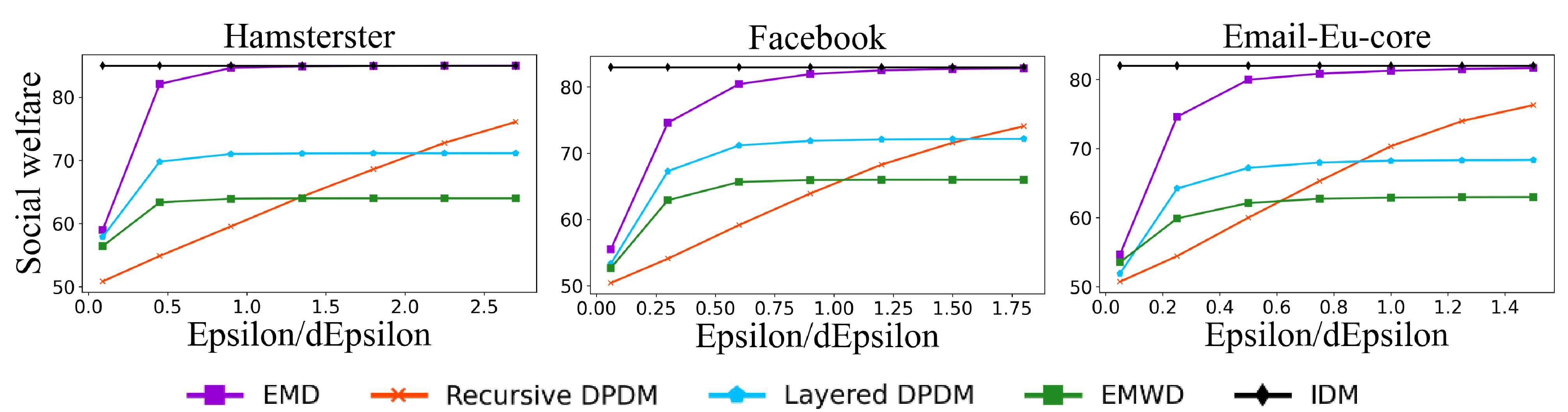
Results. Overall, when comparing to IDM, the difference in social welfare of the DPDMs decreases with $\epsilon$ increases. Then, among DPDMs, EMD performs best in most cases, followed by ${\mathrm{REC}}$ and ${\mathrm{LAY}}$ . Particularly, ${\mathrm{REC}}$ performs very well. The lines of ${\mathrm{REC}}$ even coincide with those of EMD in some cases, e.g., on Facebook & Email-Eu-core in Fig. 2. The deviation of ${\mathrm{REC}}$ from EMD is at most $2.62\%$ . ${\mathrm{REC}}$ performs better than the layered counterpart. EMWD returns the worst expected social welfare. The reason why ${\mathrm{REC}}$ has better expected social welfare than ${\mathrm{LAY}}$ is that in ${\mathrm{LAY}}$ , a probability of $1-\sum_{\ell=1}^{d_{\max}}\gamma_{\ell}$ is not distributed to any buyer, which means that the seller does not sell the item and the social welfare is $0$ with this probability.

Next we show the effect of different parameters. (1) Dataset. As shown in each column of Fig. 2, the same pattern can be found for different datasets. (2) Privacy parameter. The expected $sw$ increases with $\epsilon$ . The less privacy is required, the less noisy is added, and thus the higher probability of returning a result with good social welfare. (3) Valuation. The $1$ st and the $2$ nd row of Fig. 2 show the results with normal and uniform distributions, resp.. Under both distributions, ${\mathrm{REC}}$ performs better than ${\mathrm{LAY}}$ . (4) Sequence. Fig. 3 shows the average social welfare is best when $a=1.5,2$ for Hamsterster and when $a=2,3$ for Facebook and Email-Eu-core. When a buyer $i$ with the highest valuation is on a deeper layer, a smaller $a$ leads to a larger probability for the layer where $i$ is and also a larger probability for $i$ . The results verify this argument. In Hamsterster (Facebook, Email-Eu-core), the buyers with the highest valuation are on the $4$ th ( $3$ rd, $2$ nd) layer. (5) same DP. Fig. 4 shows when the realised privacy is large, the avg. social welfare of ${\mathrm{REC}}$ is greater than that of ${\mathrm{LAY}}$ , while when the realised privacy is small, ${\mathrm{LAY}}$ is better.

7 Conclusion and future work

We consider the problem of designing diffusion auction mechanisms that sells a single item on social networks while preserving valuation privacy. We propose two DPDMs, recursive DPDM and layered DPDM. Also, we theoretically show their incentive and privacy properties and empirically show their good performances in social welfare. We could extend this study by considering the following questions: (1) How to design a DPDM for multi-item auctions? (2) How to design a DPDM that preserves both valuation and neighbourhood privacy? and (3) How to design a DPDM that is group IC where no group of buyers can benefit from joint misreporting?

References

Archer and Tardos [2001] Aaron Archer and Éva Tardos. Truthful mechanisms for one-parameter agents. Proceedings 2001 IEEE International Conference on Cluster Computing, pages 482–491, 2001.
Bulow and Klemperer [1996] Jeremy Bulow and Paul Klemperer. Auctions versus negotiations. The American Economic Review, 86(1):180–194, 1996.
Diana et al. [2020] Emily Diana, Hadi Elzayn, Michael Kearns, Aaron Roth, Saeed Sharifi-Malvajerdi, and Juba Ziani. Differentially private call auctions and market impact. In Proceedings of the 21st ACM Conference on Economics and Computation, page 541–583, 2020.
Dwork [2008] Cynthia Dwork. Differential privacy: A survey of results. In International conference on theory and applications of models of computation, pages 1–19. Springer, 2008.
Dwork et al. [2006] Cynthia Dwork, Frank McSherry, Kobbi Nissim, and Adam Smith. Calibrating noise to sensitivity in private data analysis. In Theory of cryptography conference, pages 265–284. Springer, 2006.
Fletcher and Islam [2019] Sam Fletcher and Md Zahidul Islam. Decision tree classification with differential privacy: A survey. ACM Computing Surveys (CSUR), 52(4):1–33, 2019.
Groves [1973] Theodore Groves. Incentives in teams. Econometrica: Journal of the Econometric Society, pages 617–631, 1973.
Huang and Kannan [2012] Zhiyi Huang and Sampath Kannan. The exponential mechanism for social welfare: Private, truthful, and nearly optimal. 2012 IEEE 53rd Annual Symposium on Foundations of Computer Science, pages 140–149, 2012.
Jian et al. [2018] Lin Jian, Yang Dejun, Li Ming, Xu Jia, and Xue Guoliang. Frameworks for privacy-preserving mobile crowdsensing incentive mechanisms. In IEEE Trans. Mob. Comput, page 1851–1864, 2018.
Kawasaki et al. [2020] Takehiro Kawasaki, Nathanaël Barrot, Seiji Takanashi, Taiki Todo, and Makoto Yokoo. Strategy-proof and non-wasteful multi-unit auction via social network. In Proceedings of the AAAI Conference on Artificial Intelligence, volume 34, pages 2062–2069, 2020.
Kunegis [2013] Jérôme Kunegis. Konect: The koblenz network collection. In Proceedings of the 22nd International Conference on World Wide Web, WWW ’13 Companion, page 1343–1350. Association for Computing Machinery, 2013. 10.1145/2487788.2488173. URL https://doi.org/10.1145/2487788.2488173.
Li et al. [2017] Bin Li, Dong Hao, Dengji Zhao, and Tao Zhou. Mechanism design in social networks. In Thirty-First AAAI Conference on Artificial Intelligence, 2017.
Li et al. [2019] Bin Li, Dong Hao, Dengji Zhao, and Makoto Yokoo. Diffusion and auction on graphs. In Proceedings of the 28th International Joint Conference on Artificial Intelligence, pages 435–441, 2019.
McAuley and Leskovec [2012] Julian McAuley and Jure Leskovec. Learning to discover social circles in ego networks. NIPS’12, page 539–547. Curran Associates Inc., 2012.
McSherry and Talwar [2007] Frank McSherry and Kunal Talwar. Mechanism design via differential privacy. In 48th Annual IEEE Symposium on Foundations of Computer Science (FOCS’07), pages 94–103. IEEE, 2007.
Ni et al. [2021] Tianjiao Ni, Zhili Chen, Lin Chen, Shun Zhang, Yan Xu, and Hong Zhong. Differentially private combinatorial cloud auction. IEEE Transactions on Cloud Computing, 2021.
Xiao [2013] David Xiao. Is privacy compatible with truthfulness? IACR Cryptol. ePrint Arch., 2011:5, 2013.
Xu et al. [2017] Jinlai Xu, Balaji Palanisamy, Yuzhe Tang, and S.D. Madhu Kumar. Pads: Privacy-preserving auction design for allocating dynamically priced cloud resources. In 2017 IEEE 3rd International Conference on Collaboration and Internet Computing (CIC), pages 87–96, 2017. 10.1109/CIC.2017.00023.
Yin et al. [2017] Hao Yin, Austin R. Benson, Jure Leskovec, and David F. Gleich. Local higher-order graph clustering. In Proceedings of the 23rd ACM SIGKDD International Conference on Knowledge Discovery and Data Mining, KDD ’17, page 555–564. Association for Computing Machinery, 2017. 10.1145/3097983.3098069. URL https://doi.org/10.1145/3097983.3098069.
Zhang et al. [2020a] Wen Zhang, Dengji Zhao, and Hanyu Chen. Redistribution mechanism on networks. In Proceedings of the 19th International Conference on Autonomous Agents and MultiAgent Systems, pages 1620–1628, 2020a.
Zhang et al. [2020b] Wen Zhang, Dengji Zhao, and Yao Zhang. Incentivize diffusion with fair rewards. In ECAI 2020, pages 251–258. IOS Press, 2020b.
Zhao et al. [2018] Dengji Zhao, Bin Li, Junping Xu, Dong Hao, and Nicholas R Jennings. Selling multiple items via social networks. In Proceedings of the 17th International Conference on Autonomous Agents and MultiAgent Systems, pages 68–76, 2018.
Zhao and Chen [2022] Ying Zhao and Jinjun Chen. A survey on differential privacy for unstructured data content. ACM Computing Surveys (CSUR), 54(10s):1–28, 2022.
Zhu and Shin [2015] Ruihao Zhu and Kang G Shin. Differentially private and strategy-proof spectrum auction with approximate revenue maximization. In 2015 IEEE conference on computer communications (INFOCOM), pages 918–926. IEEE, 2015.
Zhu et al. [2014] Ruihao Zhu, Zhijing Li, Fan Wu, Kang Shin, and Guihai Chen. Differentially private spectrum auction with approximate revenue maximization. In Proceedings of the 15th ACM international symposium on mobile ad hoc networking and computing, pages 185–194, 2014.

Appendix

Appendix A IDM

Here, we introduce the first diffusion auction for selling single item, IDM [13]. A key concept of IDM is diffusion critical sequence. Given a profile digraph $G_{\theta^{\prime}}$ , for any buyers $i,j\in V_{\theta^{\prime}}$ , $i$ is $\theta^{\prime}$ -critical to $j$ , denoted by $i\preceq_{\theta^{\prime}}j$ , if all paths from $s$ to $j$ in $G_{\theta^{\prime}}$ go through $i$ . A diffusion critical sequence of $i$ , denoted by $C_{i}$ , is a sequence of all diffusion critical nodes of $i$ and $i$ itself ordered by $\theta^{\prime}$ -critical relation. That is, $C_{i}=(x_{1},x_{2}\ldots,x_{k},i)$ , where $x_{1}\preceq_{\theta^{\prime}}x_{2}\preceq_{\theta^{\prime}}\ldots\preceq_{\theta^{\prime}}x_{k}\preceq_{\theta^{\prime}}i$ . Based on this concept, IDM works as follows. IDM first locates the buyer $m$ with the highest valuation among all buyers. Then it allocates the item to the buyer $w$ , who has the highest valuation when the buyers after $w$ are not considered. The winner $w$ pays the highest bid without her participation, and each diffusion critical node is rewarded by the increased payment due to her participation.

Appendix B Proof of Lemma 4.6

Lemma 4.6. Given a reported global profile $\theta^{\prime}$ , recursive DPDM ${\mathrm{REC}}$ is $\epsilon d_{\max}\Delta\sigma$ -differential privacy, where $\epsilon$ is the privacy parameter to ${\mathrm{REC}}$ .

Proof.

Given two reported global profiles $\theta$ and $\theta^{\prime}$ that differ in an arbitrary buyer $i$ ’s reported valuation such that $i$ reports $v_{i}$ in $\theta$ and $v_{i}^{\prime}$ in $\theta^{\prime}$ , we consider the probabilities that $M(\theta)$ and $M(\theta^{\prime})$ return a winner $w$ . In a critical diffusion tree $T_{\theta}$ , let $d_{w}$ denote the depth of $w$ , $a_{w}^{\ell}$ be an ancestor of $w$ with distance $\ell$ . Also, let $\mathrm{Exp}^{\theta}(T(a_{w}^{1})-T(w))$ and $\mathrm{Exp}^{\theta^{\prime}}(T(a_{w}^{1})-T(w))$ denote the value derived from $\theta$ and $\theta^{\prime}$ , respectively. Then by Equation (3), we have

	$\displaystyle\frac{\mathrm{Pr}[M(\theta)=o_{w}]}{\mathrm{Pr}[M(\theta^{\prime})=o_{w}]}$	$\displaystyle=\frac{\frac{\mathrm{Exp}(w)}{\mathrm{Exp}^{\theta}(T(a_{w}^{1})-T(w))}}{\frac{\mathrm{Exp}^{\theta^{\prime}}(w)}{\mathrm{Exp}^{\theta^{\prime}}(T(a_{w}^{1})-T(w))}}$
		$\displaystyle\times\frac{\mathrm{Pr}^{\theta}_{T[a_{w}^{1}]}-\mathrm{Pr}^{\theta}_{a_{w}^{1}}}{\mathrm{Pr}^{\theta^{\prime}}_{T[a_{w}^{1}]}-\mathrm{Pr}^{\theta^{\prime}}_{a_{w}^{1}}}$

\displaystyle\frac{\mathrm{Pr}[M(\theta)=o_{w}]}{\mathrm{Pr}[M(\theta^{\prime})=o_{w}]}=\frac{B_{0}^{\theta}}{B_{0}^{\theta^{\prime}}}\times\prod_{\ell=1}^{d_{w}-1}{\frac{A^{\theta}_{\ell}-B^{\theta}_{\ell}}{A^{\theta^{\prime}}_{\ell}-B^{\theta^{\prime}}_{\ell}}}

Next we show for each $0\leq\ell<d_{w}$ , $\frac{A^{\theta}_{\ell}-B^{\theta}_{\ell}}{A^{\theta^{\prime}}_{\ell}-B^{\theta^{\prime}}_{\ell}}$ is bounded by $\exp(\epsilon\Delta\sigma)$ . To prove it, we first show for for each $\ell$ , $(A^{\theta}_{\ell}-A^{\theta^{\prime}}_{\ell})\times(B^{\theta}_{\ell}-B^{\theta^{\prime}}_{\ell})\geq 0$ by cases.
(1) When $i\in T[a_{w}^{\ell}]$ , we have $A^{\theta}_{\ell}-A^{\theta^{\prime}}_{\ell}\leq 0,B^{\theta}_{\ell}-B^{\theta^{\prime}}_{\ell}\leq 0$ or $A^{\theta}_{\ell}-A^{\theta^{\prime}}_{\ell}\geq 0,B^{\theta}_{\ell}-B^{\theta^{\prime}}_{\ell}\geq 0$
(2) When $i\in T[a_{w}^{\ell+1}]\setminus T[a_{w}^{\ell}]$ , then $A^{\theta}_{\ell}-A^{\theta^{\prime}}_{\ell}\leq 0,B^{\theta}_{\ell}-B^{\theta^{\prime}}_{\ell}\leq 0$ or $A^{\theta}_{\ell}-A^{\theta^{\prime}}_{\ell}\geq 0,B^{\theta}_{\ell}-B^{\theta^{\prime}}_{\ell}\geq 0$
(3) When $i\notin T[a_{w}^{\ell+1}]$ , then $A^{\theta}_{\ell}-A^{\theta^{\prime}}_{\ell}=0,B^{\theta}_{\ell}-B^{\theta^{\prime}}_{\ell}=0$ .

Without loss of generality, we assume that $A^{\theta^{\prime}}_{\ell}=\alpha_{1}A^{\theta}_{\ell},B^{\theta^{\prime}}_{\ell}=\alpha_{2}B^{\theta}_{\ell},\alpha_{1},\alpha_{2}\in\mathbb{R}^{+}$ . Plug in these two equations, and we get

\frac{A^{\theta}_{\ell}-B^{\theta}_{\ell}}{A^{\theta^{\prime}}_{\ell}-B^{\theta^{\prime}}_{\ell}}=\frac{A^{\theta}_{\ell}-B^{\theta}_{\ell}}{\alpha_{1}A^{\theta}_{\ell}-\alpha_{2}B^{\theta}_{\ell}}.

Then we consider two cases:
(1) When $\alpha_{1}\geq\alpha_{2}$ , we have $\frac{A^{\theta}_{\ell}-B^{\theta}_{\ell}}{\alpha_{1}A^{\theta}_{\ell}-\alpha_{2}B^{\theta}_{\ell}}\leq\frac{A^{\theta}_{\ell}-B^{\theta}_{\ell}}{\alpha_{1}A^{\theta}_{\ell}-\alpha_{1}B^{\theta}_{\ell}}\leq\frac{1}{\alpha_{1}}.$
(2) When $\alpha_{2}\geq\alpha_{1}$ , we have $\frac{A^{\theta}_{\ell}-B^{\theta}_{\ell}}{\alpha_{1}A^{\theta}_{\ell}-\alpha_{2}B^{\theta}_{\ell}}\leq\frac{A^{\theta}_{\ell}-B^{\theta}_{\ell}}{\alpha_{2}A^{\theta}_{\ell}-\alpha_{2}B^{\theta}_{\ell}}\leq\frac{1}{\alpha_{2}}.$

After that, we show that both $\frac{1}{\alpha_{1}}$ and $\frac{1}{\alpha_{2}}$ are bounded by $\exp(\epsilon\Delta\sigma)$ as follows. By definition of $\alpha_{1}$ , we have $\frac{1}{\alpha_{1}}=\frac{A^{\theta}_{\ell}}{A^{\theta^{\prime}}_{\ell}}=\frac{\mathrm{Exp}^{\theta}(T[a_{w}^{\ell}])}{\mathrm{Exp}^{\theta^{\prime}}(T[a_{w}^{\ell}])}$ $\times\frac{\mathrm{Exp}^{\theta^{\prime}}(T(a_{w}^{\ell+1}))}{\mathrm{Exp}^{\theta}(T(a_{w}^{\ell+1}))}$ .
(1) When valuation $v_{i}^{\prime}\leq v_{i}$ , the second ratio is at most $1$ . Then we have

	$\displaystyle\frac{1}{\alpha_{1}}$	$\displaystyle=\frac{A^{\theta}_{\ell}}{A^{\theta^{\prime}}_{\ell}}\leq\frac{\mathrm{Exp}^{\theta}(T[a_{w}^{\ell}])}{\mathrm{Exp}^{\theta^{\prime}}(T[a_{w}^{\ell}])}$
		$\displaystyle\leq\frac{\sum_{k\in T[a_{w}^{\ell}]}\exp(\epsilon\sigma(\theta,o_{k}))}{\sum_{k\in T[a_{w}^{\ell}]}\exp(\epsilon(\sigma(\theta,o_{k})-\Delta\sigma))}\leq\exp(\epsilon\Delta\sigma)$

(2) When valuation $v_{i}^{\prime}\geq v_{i}$ , the first ratio is at most $1$ . We have

	$\displaystyle\frac{1}{\alpha_{1}}$	$\displaystyle=\frac{A^{\theta}_{\ell}}{A^{\theta^{\prime}}_{\ell}}\leq\frac{\mathrm{Exp}^{\theta^{\prime}}(T(a_{w}^{\ell+1}))}{\mathrm{Exp}^{\theta}(T(a_{w}^{\ell+1}))}$
		$\displaystyle\leq\frac{\sum_{k\in T(a_{w}^{\ell+1})}\exp(\epsilon(\sigma(\theta,o_{k})+\Delta\sigma))}{{\sum_{k\in T(a_{w}^{\ell+1})}\exp(\epsilon\sigma(\theta,o_{k}))}}\leq\exp(\epsilon\Delta\sigma)$

In a similar way, we can show that $\frac{1}{\alpha_{2}}\leq\exp(\epsilon\Delta\sigma)$ .

Therefore we have

	$\displaystyle\frac{\mathrm{Pr}[M(\theta)=o_{w}]}{\mathrm{Pr}[M(\theta^{\prime})=o_{w}]}$	$\displaystyle\leq\exp(\epsilon\Delta\sigma)\times\prod_{1\leq\ell<d_{w}}\exp(\epsilon\Delta\sigma)$
		$\displaystyle\leq\exp(\epsilon d_{w}\Delta\sigma)\leq\exp(\epsilon d_{\max}\Delta\sigma)$

∎

Appendix C Proof of Lemma 5.3

Lemma 5.3. Layered DPDM ${\mathrm{LAY}}$ is individually rational in terms of both valuations and neighbours.

Proof.

Given a global profile $\theta$ , for each buyer $i$ with $(v_{i},r_{i})$ , we have

	$\displaystyle\mathbf{E}_{{\mathrm{LAY}}}[u_{i}(\theta)]$	$\displaystyle=(v_{i}-p_{i}(\theta))\mathrm{Pr}_{i}(\theta_{i})$
		$\displaystyle=\int_{0}^{v_{i}}\mathrm{Pr}_{i}^{{\mathrm{LAY}}}((x,r_{i}))dx\geq 0.$

Therefore, the lemma holds. ∎

Appendix D Proof of Lemma 5.4

Lemma 5.4. Given a reported global profile $\theta^{\prime}$ , layered DPDM ${\mathrm{LAY}}$ is $\epsilon\Delta\sigma$ -differential private, where $\epsilon$ is the privacy parameter of ${\mathrm{LAY}}$ .

Proof.

Without loss of generality, we assume that $w$ is in $L_{\ell}$ , then we have

	$\displaystyle\frac{\mathrm{Pr}[M(\theta)=o_{w}]}{\mathrm{Pr}[M(\theta^{\prime})=o_{w}]}$	$\displaystyle=\frac{\mathrm{Pr}_{L_{\ell}}\times\frac{\mathrm{Exp}^{\theta}(w)}{\mathrm{Exp}^{\theta}(L_{\ell})}}{\mathrm{Pr}_{L_{\ell}}\times\frac{\mathrm{Exp}^{\theta^{\prime}}(w)}{\mathrm{Exp}^{\theta^{\prime}}(L_{\ell})}}$
		$\displaystyle=\frac{\mathrm{Exp}^{\theta}(w)}{\mathrm{Exp}^{\theta^{\prime}}(w)}\frac{\mathrm{Exp}^{\theta^{\prime}}(L_{\ell})}{\mathrm{Exp}^{\theta}(L_{\ell})}$

When $i$ is not on layer $L_{\ell}$ , $\frac{\mathrm{Pr}[M(\theta)=o_{w}]}{\mathrm{Pr}[M(\theta^{\prime})=o_{w}]}=1\leq\exp(\epsilon\Delta\sigma)$ . Otherwise, when $i$ is on layer $L_{\ell}$ , we consider two cases.
(1) $v_{i}<v_{i}^{\prime}$ . As $\sigma(\cdot)$ is non-decreasing in $v_{i}$ , the first ratio is at most $1$ . Then we have

	$\displaystyle\frac{\mathrm{Pr}[M(\theta)=o_{w}]}{\mathrm{Pr}[M(\theta^{\prime})=o_{w}]}$	$\displaystyle\leq\frac{\mathrm{Exp}^{\theta^{\prime}}(L_{\ell})}{\mathrm{Exp}^{\theta}(L_{\ell})}$
		$\displaystyle\leq\frac{\sum_{j\in L_{\ell}}\exp(\epsilon(\sigma(\theta,o_{j})+\Delta\sigma))}{\sum_{j\in L_{\ell}}\exp(\epsilon\sigma(\theta,o_{j}))}$
		$\displaystyle\leq\exp(\epsilon\Delta\sigma)$

(2) $v_{i}>v_{i}^{\prime}$ . In this case, the second ratio is at most $1$ . Then we have

	$\displaystyle{\frac{\mathrm{Pr}[M(\theta)=o_{w}]}{\mathrm{Pr}[M(\theta^{\prime})=o_{w}]}}$	$\displaystyle\leq\frac{\mathrm{Exp}^{\theta}(w)}{\mathrm{Exp}^{\theta^{\prime}}(w)}\leq\frac{\exp(\epsilon\sigma(\theta,o_{w}))}{\exp(\epsilon(\sigma(\theta,o_{w})-\Delta\sigma))}$
		$\displaystyle\leq\exp(\epsilon\Delta\sigma)$

∎

Appendix E Proof of Theorem 5.6

Theorem 5.6 Given a global profile $\theta$ , the expected social welfare of layered DPDM ${\mathrm{LAY}}$ is at least $\gamma_{d_{\max}}{\mathbf{E}_{{\mathrm{EMD}}}[sw_{{\mathrm{EMD}}}(\theta)]}$ .

Proof.

Given a global profile $\theta$ , the expected social welfare of ${\mathrm{LAY}}$ is

	$\displaystyle\mathbf{E}_{{\mathrm{LAY}}}[sw_{{\mathrm{LAY}}}(\theta)]$	$\displaystyle=\sum_{i\in V}{\left(v_{i}\times\mathrm{Pr}^{{\mathrm{LAY}}}_{i}(\theta_{i})\right)}$
		$\displaystyle=\sum_{i\in V}{v_{i}\frac{\exp(\epsilon,\sigma(\theta,o_{i}))}{\sum_{j\in L_{d_{i}}}{\frac{1}{\gamma_{d_{i}}}}\exp(\epsilon,\sigma(\theta,o_{j}))}}$
		$\displaystyle\geq\gamma_{d_{\max}}\sum_{i\in N}{v_{i}\frac{\exp(\epsilon,\sigma(\theta,o_{i}))}{\sum_{j\in L_{d_{i}}}{\exp(\epsilon,\sigma(\theta,o_{j}))}}}$
		$\displaystyle\geq\gamma_{d_{\max}}\sum_{i\in N}{v_{i}\frac{\exp(\epsilon,\sigma(\theta,o_{i}))}{\sum_{j\in V}{\exp(\epsilon,\sigma(\theta,o_{j}))}}}$
		$\displaystyle=\gamma_{d_{\max}}\mathbf{E}_{{\mathrm{LAY}}}[sw_{{\mathrm{LAY}}}(\theta)]$

∎