跳到论文正文
W Papers独立论文阅读器 arXiv:2302.07049 论文正文 计算阅读时间 · 0%
引用这篇论文根据当前论文元数据生成,正式投稿前建议核对。


License: arXiv.org perpetual non-exclusive license
arXiv:2302.07049v1 [math.OC] 14 Feb 2023

Multilevel Objective-Function-Free Optimization
with an Application to Neural Networks Training

Serge Gratton11 1 Université de Toulouse, INP, IRIT, Toulouse, France. Work partially supported by 3IA Artificial and Natural Intelligence Toulouse Institute (ANITI), French “Investing for the Future - PIA3” program under the Grant agreement ANR-19-PI3A-0004. Email: serge.gratton@enseeiht.fr.    Alena Kopaničáková22 2 Division of Applied Mathematics, Brown University, Providence, USA. Email: alena_kopanicakova@brown.edu.    Philippe L. Toint33 3 Namur Center for Complex Systems (naXys), University of Namur, Namur, Belgium. Email: philippe.toint@unamur.be.
3 II 2023
Abstract

A class of multi-level algorithms for unconstrained nonlinear optimization is presented which does not require the evaluation of the objective function. The class contains the momentum-less AdaGrad method as a particular (single-level) instance. The choice of avoiding the evaluation of the objective function is intended to make the algorithms of the class less sensitive to noise, while the multi-level feature aims at reducing their computational cost. The evaluation complexity of these algorithms is analyzed and their behaviour in the presence of noise is then illustrated in the context of training deep neural networks for supervised learning applications.

Keywords: nonlinear optimization, multilevel methods, objective-function-free optimization (OFFO), complexity, neural networks, deep learning.

1 Introduction

In many cases, optimization problems involving a large number of variables do exhibit some kind of structure, be it sparsity of derivatives [3, 5, 17, 37, 48, 49], specific invariance properties [10, 19, 21, 28, 40] or implicit spectral properties [4, 20, 26, 27, 36, 39, 41], to cite three cases of interest. If the problem arises from the discretization of an underlying infinite-dimensional setting, it has long been known that considering different discretizations of the same problem using different mesh sizes and carefully using them in what is called a multi-level or multigrid algorithm can bring substantial computational benefits. When this is the case, the remarkable numerical performance is typically obtained by exploiting the natural hierarchy between these discretizations to successively eliminate the various frequency components of the error (or residual) [6] while, at the same time, using the fact that evaluations of functions and derivatives are typically cheaper for coarse discretizations than for fine ones. Multigrid methods are now a well-researched area of numerical analysis and are viewed as a crucial tool for the solution of linear and nonlinear systems resulting from the solution of elliptic partial-differential equations. Similar ideas have also made their way in nonlinear optimization, where both the MG-Opt [39, 41] and RMTR [26] multi-level frameworks have been designed to exploit the same properties, often very successfully (see [38, 25], for instance).

Another approach of optimization for large problems has recently been explored extensively, promoting the use of very simple first-order methods (see, among many others, [14, 47, 33, 45, 52, 24]). These methods have a very low computational cost per iterations, but typically require a (sometimes very) large number of them. Their popularity relies on several facts. The first is that they can be shown to be convergent with a global rate which is sometimes comparable to that of more complicated methods. The second is that simplicity is achieved by avoiding the computation of the objective-function values and, most commonly, of other derivatives than gradients (hence their name). This in turn has made them very robust in the presence of noise on the function and its derivatives [22], an important feature when the problem is so large that these quantities can only be realistically estimated (typically by sampling) rather than calculated exactly. The context in which optimization is performed with computing function values is sometimes denoted by OFFO (Objective-Function-Free Optimization). A very large number of first-order OFFO methods have been investigated, but, for the purpose of this paper, we will focus on AdaGrad [14], one of the best-known provably-convergent members of this class.

The purpose of this paper is to demonstrate that it is possible, theoretically sound, and practically efficient to combine multi-level and OFFO algorithms. We achieve these objectives by presenting our contributions in three steps.

  • •

    We first describe a novel class of multi-level OFFO algorithms (of which AdaGrad can be viewed as a single-level realization) (Section 2).

  • •

    We then analyze the global rate of convergence of algorithms in this class, showing results matching the state of the art (Sections 3 and 4).

  • •

    We finally illustrate the use and advantages of the proposed methods in the context of noisy optimization problems resulting from the training of deep neural nets (DNNs) for supervised learning applications (Section 5).

A brief conclusion is then proposed in Section 6.

Notation.

The symbol ∥⋅∥\|\cdot\| stands for the standard Euclidean norm. If xx is a vector, |x||x| is the vector whose jj-th component is |xj||x_{j}|. The singular values of the matrix MM are denoted by σi​[M]\sigma_{i}[M].

2 The class of multilevel OFFO algorithms

We now present an idealized multilevel OFFO framework merging ideas from [23] and [26] and its analysis. The problem we consider is a structured version of smooth unconstrained optimization, that is

minx∈IRn⁡f⁡(x)\min_{x\in\hbox{\footnotesize I\hskip-2.0ptR}^{n}}f(x) (1)

for a twice continuously differentiable function ff from IRn\hbox{I\hskip-2.0ptR}^{n} into IR. The problem is structured in that we assume that we know a collection of functions which provide a “hierarchical” set of approximations of the objective function ff. As indicated above, this is typically the case when considering a function of a continuous problem’s discretization (the hierarchy being then given by varying the discretization mesh) or when the objective function involves a graph whose description may vary in its level of detail. More specifically, we assume that we know a collection of functions {fℓ}ℓ=1r\{f_{\ell}\}_{\ell=1}^{r} such that each fℓf_{\ell} is a twice-continuously differentiable function from IRnℓ\hbox{I\hskip-2.0ptR}^{n_{\ell}} to IR, the connection with our original problem being that nr=nn_{r}=n and fr​(x)=f​(x)f_{r}(x)=f(x) for all x∈IRnx\in\hbox{I\hskip-2.0ptR}^{n}. We also assume that, for each ℓ=2,…,r\ell=2,\ldots,r, fℓf_{\ell} is “more costly” to evaluate/minimize than fℓ−1f_{\ell-1}. This may be because fℓf_{\ell} has more variables than fℓ−1f_{\ell-1} (as would typically be the case if the fℓf_{\ell} represent increasingly finer discretizations of the same infinite-dimensional objective), or because the structure (in terms of partial separability, sparsity or eigenstructure) of fℓf_{\ell} is more complex than that of fℓ−1f_{\ell-1}, or for any other reason. To fix terminology, we will refer to a particular ℓ\ell as a level. However, for fℓ−1f_{\ell-1} to be useful at all in minimizing fℓf_{\ell}, there should be some relation between the variables of these two functions. We thus assume that, for each ℓ=2,…,r\ell=2,\ldots,r, there exist a full-rank linear operator RℓR_{\ell} from IRnℓ\hbox{I\hskip-2.0ptR}^{n_{\ell}} into IRnℓ−1\hbox{I\hskip-2.0ptR}^{n_{\ell-1}} (the restriction) and another full-rank operator PℓP_{\ell} from IRnℓ−1\hbox{I\hskip-2.0ptR}^{n_{\ell-1}} into IRnℓ\hbox{I\hskip-2.0ptR}^{n_{\ell}} (the prolongation) such that

ω​Pℓ=RℓT\omega P_{\ell}=R_{\ell}^{T} (2)

for some known constant** * For simplicity, we choose to make ω\omega independent of ℓ\ell, which can always be achieved by scaling. ω>0\omega>0. In the context of multigrid algorithms, PℓP_{\ell} and RℓR_{\ell} are interpreted as restriction and prolongation between a fine and a coarse grid (see [6, 41, 26, 25], for instance).

Before going into further details, we establish an important convention on indices. Since we will have to identify, sometimes simultaneously, a level, an iteration of our algorithm and a vector’s component, we associate the index ℓ\ell with levels, ii with iterations and jj with components. For instance, xℓ,i,jx_{\ell,i,j} stands for the jj-th component of the vector xx at iteration ii within level ℓ\ell. The iteration index ii will be reset to zero each time a level is entered†† † We are well aware that this creates some ambiguities, since a sequence of indices ℓ,i\ell,i can occur more than once if level ℓ\ell (ℓ<r\ell<r) is used more than once, implying the existence of more than one starting iterate at this level. This ambiguity is resolved by the context..

Because our proposal is to extend the ASTR1 objective-function-free framework of [23] to the multilevel context, we now review the main concepts of this algorithm and establish some notation. As the TR in the name suggests, ASTR1 is a trust-region optimization algorithm. This class of algorithms is well-known to be both theoretically sound (see [11] for an in-depth presentation and [51] for a more recent survey) and practically very efficient. As in all trust-region methods, the next iterate at level ℓ\ell is found by minimizing a model of a level-dependent objective function hℓh_{\ell} within a region where the model is trusted. In our multilevel framework, this model can be either the (potentially quadratic) Taylor-like

mℓ,i​(s)=gℓ,iT​s+12​sT​Bℓ,i​s,m_{\ell,i}(s)=g_{\ell,i}^{T}s+{\scriptstyle\frac{1}{2}}s^{T}B_{\ell,i}s, (3)

where gℓ,i=def∇x1​hℓ​(xℓ,i)g_{\ell,i}\stackrel{{\scriptstyle\rm def}}{{=}}\nabla_{x}^{1}h_{\ell}(x_{\ell,i}) and Bℓ,iB_{\ell,i} is a bounded Hessian approximation, or the lower level model defined by

hℓ−1​(xℓ−1,0+sℓ−1)=deffℓ−1​(xℓ−1,0+sℓ−1)+vℓ−1T​sℓ−1,h_{\ell-1}(x_{\ell-1,0}+s_{\ell-1})\stackrel{{\scriptstyle\rm def}}{{=}}f_{\ell-1}(x_{\ell-1,0}+s_{\ell-1})+v_{\ell-1}^{T}s_{\ell-1}, (4)

where

vℓ−1=Rℓ​gℓ,i−∇fℓ−1​(xℓ−1,0).v_{\ell-1}=R_{\ell}g_{\ell,i}-\nabla f_{\ell-1}(x_{\ell-1,0}). (5)

By convention, we set vr=0v_{r}=0, so that, for all srs_{r},

hr​(xr,0+sr)=fr​(xr,0+sr)=f⁡(xr,0+sr)​and​gr,k=∇x1hr​(xr,k)=∇x1f​(xr,k).h_{r}(x_{r,0}+s_{r})=f_{r}(x_{r,0}+s_{r})=f(x_{r,0}+s_{r})\;\;\mbox{and}\;\;g_{r,k}=\nabla_{x}^{1}h_{r}(x_{r,k})=\nabla_{x}^{1}f(x_{r,k}). (6)

The model hℓh_{\ell} therefore corresponds to a modification of fℓf_{\ell} by a linear term that enforces the “linear coherence” relation

gℓ−1,0=∇x1​hℓ−1​(xℓ−1,0)=Rℓ​gℓ,i.g_{\ell-1,0}=\nabla_{x}^{1}h_{\ell-1}(x_{\ell-1,0})=R_{\ell}g_{\ell,i}. (7)

This first-order modification (4) is commonly used in multigrid applications in the context of the full approximation scheme [6], but also in other contexts [16, 41, 1, 38, 26, 34]. We call it “linear coherence” because it crucially ensures that the first-order behaviours of hℓh_{\ell} and hℓ−1h_{\ell-1} are coherent in a neighbourhood of xℓ,ix_{\ell,i} and xℓ−1,0x_{\ell-1,0}, respectively. To see this, one checks that, if sℓs_{\ell} and sℓ−1s_{\ell-1} satisfy sℓ=Pℓ​sℓ−1,s_{\ell}=P_{\ell}s_{\ell-1}, then, using (2) and (7),

gℓ,iT​sℓ=gℓ,iT​Pℓ​si−1=1ω​Rℓ​gℓ,iT​sℓ−1=1ω​gℓ−1,0T​sℓ−1.g_{\ell,i}^{T}s_{\ell}=g_{\ell,i}^{T}P_{\ell}s_{i-1}=\frac{1}{\omega}R_{\ell}g_{\ell,i}^{T}s_{\ell-1}=\frac{1}{\omega}g_{\ell-1,0}^{T}s_{\ell-1}. (8)

Once the model is defined/chosen, the typical iteration of a trust-region method proceeds by minimizing it in a ball centered at the current iterate, whose radius is adaptively computed by the algorithm, depending on past performance. This ball can be defined in different norms, but we will focus here on a scaled version of the “infinity norm” where the absolute value of each vector component is measured individually. In the ASTR1 context, the trust-region radius is computed using the size of the current gradient and a component-wise strictly positive vector of weights, which we do not fully define now, but which will be specified later in our analysis. Since our multilevel algorithm is recursive, it is also necessary to force termination at a given level when the Euclidean norm of the prolongation of the overall step to the previous level becomes too large, that is when the inequality

‖Pℓ+1​(xℓ,i−xℓ,0)‖≤δℓ\|P_{\ell+1}(x_{\ell,i}-x_{\ell,0})\|\leq\delta_{\ell} (9)

fails, where δℓ≥0\delta_{\ell}\geq 0 is a bound on norm of the step at level ℓ+1\ell+1 if ℓ<r\ell<r or +∞+\infty otherwise.

In order to specify the algorithm, we finally define, for a vector of weights wℓw_{\ell} of size nℓn_{\ell}, the diagonal matrices

D⁡({wℓ})=defdiag⁡(1wℓ,1,…,1wℓ,nℓ).D(\{w_{\ell}\})\stackrel{{\scriptstyle\rm def}}{{=}}{\rm diag}\left(\frac{1}{w_{\ell,1}},\ldots,\frac{1}{w_{\ell,n_{\ell}}}\right). (10)

We will assume that, for j∈{1,…,nℓ}j\in\{1,\ldots,n_{\ell}\}, there exists a constant ςj∈(0,1]\varsigma_{j}\in(0,1], such that wℓ,j≥ςjw_{\ell,j}\geq\varsigma_{j} for each ℓ∈{1,…,r}\ell\in\{1,\ldots,r\}. The Multilevel Objective-Function-Free Trust-Region (MOFFTR) algorithm is then specified 2.

Solving the original problem (1) is then obtained by calling

𝖬𝖮𝖥𝖥𝖳𝖱⁡(r,f,xr,0,ϵr,ir(max),+∞,ς),{\footnotesize{\sf MOFFTR}}(\,r,\,f,\,x_{r,0},\,\epsilon_{r},\,i^{(\max)}_{r},\,+\infty,\,\varsigma\,), (11)

where ir(max)i^{(\max)}_{r} is the maximum number of top level iterations and ς\varsigma denotes the vector of weights’ lower bounds. In order to fix terminology, we say that iterations at which the step is computed by Step 4 of the algorithm are Taylor iterations, while iterations at which the step results from the recursive call (17) are called recursive iterations.

Algorithm 2.1:        x+=𝖬𝖮𝖥𝖥𝖳𝖱⁡(ℓ,hℓ,xℓ,0,ϵℓ,iℓ(max),δℓ,wℓ,0)x_{+}={\footnotesize{\sf MOFFTR}}(\ell,h_{\ell},x_{\ell,0},\epsilon_{\ell},i_{\ell}^{(\max)},\delta_{\ell},w_{\ell,0})
Step 0: Initialization. The constants κR∈(0,1)\kappa_{\mbox{\tiny R}}\in(0,1), α≥1\alpha\geq 1, τ∈(0,1]\tau\in(0,1], κB≥1\kappa_{\mbox{\tiny B}}\geq 1 and ςj∈(0,1]\varsigma_{j}\in(0,1] (OPENj∈{1,…,nℓ})j\in\{1,\ldots,n_{\ell}\}) are given. Set i=0i=0. Step 1: Termination test. If ℓ<r\ell<r and ‖Pℓ+1​(xℓ,i−xℓ,0)‖>δℓ\|P_{\ell+1}(x_{\ell,i}-x_{\ell,0})\|>\delta_{\ell} (12) return with x+=xℓ,i−1x_{+}=x_{\ell,i-1}. Otherwise, compute gℓ,i=def∇x1​hℓ​(xℓ,i)g_{\ell,i}\stackrel{{\scriptstyle\rm def}}{{=}}\nabla_{x}^{1}h_{\ell}(x_{\ell,i}). If ‖gℓ,i‖≤ϵℓ\|g_{\ell,i}\|\leq\epsilon_{\ell} or i=iℓ(max)i=i_{\ell}^{(\max)}, return with x+=xℓ,ix_{+}=x_{\ell,i}. Step 2: Define the trust-region. Set Δ^ℓ,i=D⁡({wℓ,i})​|gℓ,i|​and​Δℓ,i={Δ^ℓ,iif ​ℓ=r,min⁡[2​δℓ‖Pℓ+1‖​‖Δ^ℓ,i‖,1]​Δ^ℓ,iif ​ℓ<r.\widehat{\Delta}_{\ell,i}=D(\{w_{\ell,i}\})|g_{\ell,i}|\;\;\mbox{and}\;\;\Delta_{\ell,i}=\left\{\begin{array}[]{ll}\widehat{\Delta}_{\ell,i}&\;\;\mbox{if }\;\;\ell=r,\\ \min\left[\frac{\displaystyle 2\delta_{\ell}}{\displaystyle\|P_{\ell+1}\|\,\|\widehat{\Delta}_{\ell,i}\|},1\right]\widehat{\Delta}_{\ell,i}&\;\;\mbox{if }\;\;\ell<r.\\ \end{array}\right. (13) If i>0i>0, define wℓ,i∈IRnℓw_{\ell,i}\in\hbox{I\hskip-2.0ptR}^{n_{\ell}} such that wℓ,i,j≥ςjw_{\ell,i,j}\geq\varsigma_{j} for j∈{1,…,nℓ}j\in\{1,\ldots,n_{\ell}\}. If a Taylor step is required at iteration ii, go to Step 4. Step 3: Recursive step. Select wℓ−1,0∈IRnℓ−1w_{\ell-1,0}\in\hbox{I\hskip-2.0ptR}^{n_{\ell-1}} such that wℓ−1,0,j≥ςjw_{\ell-1,0,j}\geq\varsigma_{j} for j∈{1,…,nℓ−1}j\in\{1,\ldots,n_{\ell-1}\},    “the lower-level weights are large enough”    (14) and ‖D⁡({wℓ−1,0})​|Rℓ​gℓ,i|‖≤α​‖Δℓ,i‖‖Pℓ‖.\left\|D(\{w_{\ell-1,0}\})\,|R_{\ell}g_{\ell,i}|\right\|\leq\frac{\alpha\|\Delta_{\ell,i}\|}{\|P_{\ell}\|}. (15) If either ℓ=1\ell=1 or ∑j=1nℓ−1[Rℓ​gℓ,i]j2wℓ−1,0,j<κR​∑j=1nℓgℓ,i,j2wℓ,i,j\sum_{j=1}^{n_{\ell}-1}\frac{[R_{\ell}g_{\ell,i}]^{2}_{j}}{w_{\ell-1,0,j}}<\kappa_{\mbox{\tiny R}}\sum_{j=1}^{n_{\ell}}\frac{g_{\ell,i,j}^{2}}{w_{\ell,i,j}} (16) then go to Step 4. Otherwise (i.e. if ℓ>1\ell>1 and (16) fails), compute sℓ,i=Pℓ​[𝖬𝖮𝖥𝖥𝖳𝖱⁡(ℓ−1,hℓ−1,Rℓ​xℓ,i,ϵℓ−1,iℓ−1(max),α​‖Δℓ,i‖,wℓ−1,0)−Rℓ​xℓ,i],s_{\ell,i}=P_{\ell}\Big[{\footnotesize{\sf MOFFTR}}(\ell-1,h_{\ell-1},R_{\ell}x_{\ell,i},\epsilon_{\ell-1},i_{\ell-1}^{(\max)},\alpha\|\Delta_{\ell,i}\|,w_{\ell-1,0})-R_{\ell}x_{\ell,i}\Big], (17) where hℓ−1h_{\ell-1} is given by (4). Step 4: Taylor step. Select a symmetric Hessian approximation Bℓ,iB_{\ell,i} such that ‖Bℓ,i‖≤κB.\|B_{\ell,i}\|\leq\kappa_{\mbox{\tiny B}}.\vskip-5.69054pt (18) Compute a step sℓ,is_{\ell,i} such that |sℓ,i,j|≤Δℓ,i,j(j∈{1,…,nℓ}),|s_{\ell,i,j}|\leq\Delta_{\ell,i,j}\;\;\;\;(j\in\{1,\ldots,n_{\ell}\}), (19) and gℓ,iT​sℓ,i+12​sℓ,iT​Bℓ,i​sℓ,i≤τ⁡(gℓ,iT​sℓ,iQ+12​(sℓ,iQ)T​Bℓ,i​sℓ,iQ),g_{\ell,i}^{T}s_{\ell,i}+{\scriptstyle\frac{1}{2}}s_{\ell,i}^{T}B_{\ell,i}s_{\ell,i}\leq\tau\left(g_{\ell,i}^{T}s_{\ell,i}^{Q}+{\scriptstyle\frac{1}{2}}(s_{\ell,i}^{Q})^{T}B_{\ell,i}s_{\ell,i}^{Q}\right), (20) where sℓ,i,jL=−sign⁡(gℓ,i,j)​Δℓ,i,j(j∈{1,…,nℓ}),s_{\ell,i,j}^{L}=-{\rm sign}(g_{\ell,i,j})\Delta_{\ell,i,j}\;\;\;\;(j\in\{1,\ldots,n_{\ell}\}), (21) sℓ,iQ=γℓ,i​sℓ,iL, with ​γℓ,i={min⁡[1,|gℓ,iT​sℓ,iL|(sℓ,iL)T​Bℓ,i​sℓ,iL]if ​(sℓ,iL)T​Bℓ,i​sℓ,iL>0,1otherwise.s^{Q}_{\ell,i}=\gamma_{\ell,i}s_{\ell,i}^{L},\;\;\mbox{ with }\;\;\gamma_{\ell,i}=\left\{\begin{array}[]{ll}\min\left[1,\frac{\displaystyle|g_{\ell,i}^{T}s_{\ell,i}^{L}|}{\displaystyle(s_{\ell,i}^{L})^{T}B_{\ell,i}s_{\ell,i}^{L}}\right]&\;\;\mbox{if }\;\;(s_{\ell,i}^{L})^{T}B_{\ell,i}s_{\ell,i}^{L}>0,\\ 1&\;\;\mbox{otherwise.}\end{array}\right. (22) Step 5: Update. Set xℓ,i+1=xℓ,i+sℓ,i,x_{\ell,i+1}=x_{\ell,i}+s_{\ell,i}, (23) Increment ii by one and return to Step 1.

Some comments are useful at this stage to further explain and motivate the details of the algorithm.

  1. 1.

    Note that the iterations at any level are terminated in Step 1 if a level-dependent accuracy threshold ϵℓ\epsilon_{\ell} is achieved or if a level-dependent maximum number of iterations iℓ(max)i_{\ell}^{(\max)} is reached. Also note that (12) enforces (9).

  2. 2.

    The componentwise trust-region radius is defined in (13). Observe that this choice prevents nonzero components of the step whenever the corresponding component of the gradient is zero. Observe also that (13) avoids large steps which would cause (12) to fail for i+1i+1. Indeed, if ℓ<r\ell<r, (13) and (19) imply that

    ‖Pℓ+1​(xℓ,i+1−xℓ,i)‖=‖Pℓ+1​sℓ,i‖≤2​δℓ.\|P_{\ell+1}(x_{\ell,i+1}-x_{\ell,i})\|=\|P_{\ell+1}s_{\ell,i}\|\leq 2\delta_{\ell}.

    Thus any xℓ,i+1x_{\ell,i+1} which would violate this inequality would not satisfy (12) (for i+1i+1) since then

    ‖Pℓ+1​(xℓ,i+1−xℓ,0)‖≥‖Pℓ+1​(xℓ,i+1−xℓ,i)‖−‖Pℓ+1​(xℓ,i−xℓ,0)‖>2​δℓ−δℓ=δℓ,\|P_{\ell+1}(x_{\ell,i+1}-x_{\ell,0})\|\geq\|P_{\ell+1}(x_{\ell,i+1}-x_{\ell,i})\|-\|P_{\ell+1}(x_{\ell,i}-x_{\ell,0})\|>2\delta_{\ell}-\delta_{\ell}=\delta_{\ell},

    where we used (12) (for ii) to derive the last inequality.

    The choice of model (end of Step 2) is not formally determined and left to the user. In a typical pattern, known in the multigrid literature as a “V-cycle”, the tasks to perform at a given level ℓ\ell is as follows. A set of standard Taylor iterations is first performed. Then, if ℓ>1\ell>1 (that is the current level is not the lowest one) and significant progress is likely on level ℓ−1\ell-1 (in the sense of (16) failing), one then recursively calls the algorithm at level ℓ−1\ell-1. A second set of Taylor iterations is then performed at level ℓ\ell. The “V” shape suggested by the name results from the recursive application of this pattern at all levels. While it is customary to specify the number of Taylor iterations in both sets (the “pre-smoothing” and “post-smoothing” in multigrid parlance), this is not required in MOFFTR. Indeed the algorithm allows for a wide variety of iteration patterns, fixed or adaptive.

  3. 3.

    We next review the mechanism of Step 3 and start by noting that δℓ,i\delta_{\ell,i} is the Euclidean norm of the step that would be allowed at iteration (ℓ,i)(\ell,i), had this iteration been been a Taylor one (see (13)). We then select a set of weights wℓ−1,0w_{\ell-1,0} to be used at the lower level. Beyond being bounded below by their respective ςj\varsigma_{j}, these weights have to satisfy two further conditions. The first, (14), is expressed in a very generic way for now and ensures that these weights cannot be small if the weights at level ℓ\ell are large. How this is achieved will depend on the specific choice of weights, as we will see below. The second is the seemingly obscure condition (15), which simply ensures that the global bound on the Euclidean norm on the total step at level ℓ−1\ell-1 is large enough to allow at least one iteration at the lower level. It states that the Euclidean length of the prolongation PℓP_{\ell} of the first lower level step is at most some multiple α≥1\alpha\geq 1 of the Euclidean length of the (hypothetical) step at level ℓ\ell. Condition (16) then compares the decrease in a linear approximation of hℓ−1h_{\ell-1} at Rℓ​xℓ,iR_{\ell}x_{\ell,i} with that of the linear approximation of hℓh_{\ell} at xℓ,ix_{\ell,i}. If the former is less than a fraction κR\kappa_{\mbox{\tiny R}} of the latter, this suggests that “significant progress at the lower level is unlikely”, and we then resort to continue minimization at the current level. If significant progress is likely, we then choose to minimize hℓ−1h_{\ell-1} at the lower level (recursive iteration) using the weights wℓ−1,0w_{\ell-1,0}, starting from Rℓ​xℓ,iR_{\ell}x_{\ell,i} and within a Euclidean ball of radius α​‖Δℓ,i‖\alpha\|\Delta_{\ell,i}\|.

    We observe that (15) is quite easy to satisfy. Indeed, one readily checks that it is guaranteed if

    wℓ−1,0,j≥max⁡[ςj,‖Pℓ‖​|Rℓ​gℓ,i|jα​‖Δℓ,i‖].w_{\ell-1,0,j}\geq\max\left[\varsigma_{j},\frac{\|P_{\ell}\|\,|R_{\ell}g_{\ell,i}|_{j}}{\alpha\|\Delta_{\ell,i}\|}\right]. (24)
  4. 4.

    The step at Taylor iterations is computed in Step 4 using a technique borrowed from the ASTR1 algorithm [23]. The reader familiar with trust-region theory will recognize in sℓ,iQs^{Q}_{\ell,i} a variant the “Cauchy point” obtained by minimizing the quadratic model on the intersection of the negative gradient’s span and the trust-region (see [11, Section 6.3.2]), while sℓ,iLs_{\ell,i}^{L} is minimizer of the simpler linear model gℓ,iT​sg_{\ell,i}^{T}s within the trust-region.

  5. 5.

    Neither the objective function frf_{r} or its approximations {fℓ}ℓ=1r−1\{f_{\ell}\}_{\ell=1}^{r-1} are ever evaluated and the optimization method combining them is therefore truly “Objective-Function-Free”.

3 Convergence Analysis

Our convergence analysis is based on the following standard assumptions.

AS.1:

For each ℓ∈{1,…,r}\ell\in\{1,\ldots,r\}, the function fℓf_{\ell} is continuously differentiable.

AS.2:

For each ℓ∈{1,…,r}\ell\in\{1,\ldots,r\}, the gradient ∇x1​fℓ​(x)\nabla_{x}^{1}f_{\ell}(x) is Lipschitz continuous with Lipschitz constant L≥0L\geq 0, that is

‖∇x1​fℓ​(x)−∇x1​fℓ​(y)‖≤L​‖x−y‖\|\nabla_{x}^{1}f_{\ell}(x)-\nabla_{x}^{1}f_{\ell}(y)\|\leq L\|x-y\|

for all x,y∈IRnx,y\in\hbox{I\hskip-2.0ptR}^{n} and all ℓ∈{1,…,r}\ell\in\{1,\ldots,r\}.

AS.3:

There exists a constant flowf_{\rm low} such that, for all xx, f⁡(x)≥flowf(x)\geq f_{\rm low}.

In what follows, we use the notation

Γ0=deff⁡(x0)−flow\Gamma_{0}\stackrel{{\scriptstyle\rm def}}{{=}}f(x_{0})-f_{\rm low} (25)

for the gap between the objective function at the starting point and its lower bound. Note that there is no assumption that the gradients of the fℓf_{\ell} remain bounded.

Before considering more specific choices for the weights, we first derive a fundamental property of the Taylor steps and strengthen [23, Lemma 2.1] quantifying the “linear decrease” (that is the decrease in the simple linear model of the objective) for Taylor iterations.

Lemma 3.1
Suppose that AS.1 and AS.2 hold. Consider a Taylor iteration ii at level ℓ\ell. Then gℓ,iTsℓ,i≤−τ​ςmin2​κB∑j=1nℓgℓ,i,j2wℓ,i,j+κB2∥Δℓ,i∥2g_{\ell,i}^{T}s_{\ell,i}\leq-\frac{\tau\varsigma_{\min}}{2\kappa_{\mbox{\tiny B}}}\sum_{j=1}^{n_{\ell}}\frac{g_{\ell,i,j}^{2}}{w_{\ell,i,j}}+\frac{\kappa_{\mbox{\tiny B}}}{2}\|\Delta_{\ell,i}\|^{2} (26) where ςmin=defminj∈{1,…,nℓ}⁡ςj∈(0,1]\varsigma_{\min}\stackrel{{\scriptstyle\rm def}}{{=}}\min_{j\in\{1,\ldots,n_{\ell}\}}\varsigma_{j}\in(0,1].

  • Proof.   First note that, because of (21) and the definition of wℓ,i,jw_{\ell,i,j},

    |gℓ,iT​sℓ,iL|=∑j=1nℓwℓ,i,j​gℓ,i,j2wℓ,i,j2≥∑j=1nℓςj​gℓ,i,j2wℓ,i,j2≥ςmin​‖sℓ,iL‖2.|g_{\ell,i}^{T}s_{\ell,i}^{L}|=\sum_{j=1}^{n_{\ell}}\frac{w_{\ell,i,j}g_{\ell,i,j}^{2}}{w_{\ell,i,j}^{2}}\geq\sum_{j=1}^{n_{\ell}}\frac{\varsigma_{j}g_{\ell,i,j}^{2}}{w_{\ell,i,j}^{2}}\geq\varsigma_{\min}\|s_{\ell,i}^{L}\|^{2}. (27)

    Suppose now that (sℓ,iL)T​Bℓ,i​sℓ,iL>0(s_{\ell,i}^{L})^{T}B_{\ell,i}s_{\ell,i}^{L}>0 and γℓ,i<1\gamma_{\ell,i}<1. Then, in view of (20), (22), (27) and (18),

    gℓ,iT​sℓ,iQ+12​(sℓ,iQ)T​Bℓ,i​sℓ,iQ=γℓ,i​gℓ,iT​sℓ,iL+12​γℓ,i2​(sℓ,iL)T​Bℓ,i​sℓ,iL=−(gℓ,iT​sℓ,iL)22​(sℓ,iL)T​Bℓ,i​sℓ,iL≤−ςmin​|gℓ,iT​sℓ,iL|2​κB.g_{\ell,i}^{T}s_{\ell,i}^{Q}+{\scriptstyle\frac{1}{2}}(s_{\ell,i}^{Q})^{T}B_{\ell,i}s_{\ell,i}^{Q}=\gamma_{\ell,i}g_{\ell,i}^{T}s_{\ell,i}^{L}+{\scriptstyle\frac{1}{2}}\gamma_{\ell,i}^{2}(s_{\ell,i}^{L})^{T}B_{\ell,i}s_{\ell,i}^{L}=-\frac{(g_{\ell,i}^{T}s_{\ell,i}^{L})^{2}}{2(s_{\ell,i}^{L})^{T}B_{\ell,i}s_{\ell,i}^{L}}\leq-\frac{\varsigma_{\min}|g_{\ell,i}^{T}s_{\ell,i}^{L}|}{2\kappa_{\mbox{\tiny B}}}.

    Combining this inequality with (22) then gives that

    gℓ,iTsℓ,iQ+12(sℓ,iQ)TBℓ,isℓ,iQ≤−ςmin2​κB∑j=1nℓgℓ,i,j2wℓ,i,j.g_{\ell,i}^{T}s_{\ell,i}^{Q}+{\scriptstyle\frac{1}{2}}(s_{\ell,i}^{Q})^{T}B_{\ell,i}s_{\ell,i}^{Q}\leq-\frac{\varsigma_{\min}}{2\kappa_{\mbox{\tiny B}}}\sum_{j=1}^{n_{\ell}}\frac{g_{\ell,i,j}^{2}}{w_{\ell,i,j}}. (28)

    Alternatively, suppose that (sℓ,iL)T​Bℓ,i​sℓ,iL≤0(s_{\ell,i}^{L})^{T}B_{\ell,i}s_{\ell,i}^{L}\leq 0 or γℓ,i=1\gamma_{\ell,i}=1. Then, using (22), (21) and bounds κB≥1\kappa_{\mbox{\tiny B}}\geq 1 and ςmin≤1\varsigma_{\min}\leq 1,

    gℓ,iTsℓ,iQ+12(sℓ,iQ)TBℓ,isℓ,iQ=gℓ,iTsℓ,iL+12(sℓ,iL)TBℓ,isℓ,iL≤12gℓ,iTsℓ,iL≤−ςmin2​κB∑j=1nℓgℓ,i,j2wℓ,i,j.g_{\ell,i}^{T}s_{\ell,i}^{Q}+{\scriptstyle\frac{1}{2}}(s_{\ell,i}^{Q})^{T}B_{\ell,i}s_{\ell,i}^{Q}=g_{\ell,i}^{T}s_{\ell,i}^{L}+{\scriptstyle\frac{1}{2}}(s_{\ell,i}^{L})^{T}B_{\ell,i}s_{\ell,i}^{L}\leq{\scriptstyle\frac{1}{2}}g_{\ell,i}^{T}s_{\ell,i}^{L}\leq-\frac{\varsigma_{\min}}{2\kappa_{\mbox{\tiny B}}}\sum_{j=1}^{n_{\ell}}\frac{g_{\ell,i,j}^{2}}{w_{\ell,i,j}}. (29)

    We thus obtain from (28), (29) and (20) that

    gℓ,i,Tsℓ,i+12sℓ,iTBℓ,isℓ,i≤−τ​ςmin2​κB∑j=1nℓgℓ,i,j2wℓ,i,j.g_{\ell,i,}^{T}s_{\ell,i}+{\scriptstyle\frac{1}{2}}s_{\ell,i}^{T}B_{\ell,i}s_{\ell,i}\leq-\frac{\tau\varsigma_{\min}}{2\kappa_{\mbox{\tiny B}}}\sum_{j=1}^{n_{\ell}}\frac{g_{\ell,i,j}^{2}}{w_{\ell,i,j}}.

    As a consequence, we deduce from (28), (29), (20) and (18) that

    gℓ,iTsℓ,i≤−τςmin∑j=1nℓgℓ,i,j22​κB​wℓ,i,j+12|sℓ,iTBℓ,isℓ,i|≤−τςmin∑j=1nℓgℓ,i,j22​κB​wℓ,i,j+κB2∑j=1nℓsℓ,i,j2,g_{\ell,i}^{T}s_{\ell,i}\leq-\tau\varsigma_{\min}\sum_{j=1}^{n_{\ell}}\frac{g_{\ell,i,j}^{2}}{2\kappa_{\mbox{\tiny B}}w_{\ell,i,j}}+{\scriptstyle\frac{1}{2}}|s_{\ell,i}^{T}B_{\ell,i}s_{\ell,i}|\leq-\tau\varsigma_{\min}\sum_{j=1}^{n_{\ell}}\frac{g_{\ell,i,j}^{2}}{2\kappa_{\mbox{\tiny B}}w_{\ell,i,j}}+\frac{\kappa_{\mbox{\tiny B}}}{2}\sum_{j=1}^{n_{\ell}}s_{\ell,i,j}^{2},

    and (26) results from (19). □\Box

We also prove the following easy lemma.

Lemma 3.2
Consider iteration (ℓ,i)(\ell,i) in the course of the MOFFTR algorithm. Then ‖sℓ,i‖≤α​‖D⁡({wℓ,i})​|gℓ,i|‖.\|s_{\ell,i}\|\leq\alpha\|D(\{w_{\ell,i}\})|g_{\ell,i}|\|. (30)

  • Proof.    If iteration (ℓ,i)(\ell,i) is a Taylor iteration, (30) results from (13), (19) and the bound α≥1\alpha\geq 1. If it is a recursive iteration, we have, from (17) and (19), that

    ‖sℓ,i‖=‖Pℓ​(xℓ−1,i−xℓ−1,0)‖≤δℓ−1=α​‖D⁡({wℓ,i})​|gℓ,i|‖,\|s_{\ell,i}\|=\|P_{\ell}(x_{\ell-1,i}-x_{\ell-1,0})\|\leq\delta_{\ell-1}=\alpha\|D(\{w_{\ell,i}\})|g_{\ell,i}|\|,

    yielding (30). □\Box

We now consider what can happen at a recursive iteration.

Lemma 3.3
Consider an recursive iteration (ℓ,i)(\ell,i). Then ‖Δℓ−1,0‖≤α‖Pℓ‖​‖Δℓ,i‖,\|\Delta_{\ell-1,0}\|\leq\frac{\alpha}{\|P_{\ell}\|}\|\Delta_{\ell,i}\|, (31) the iterate xℓ−1,1x_{\ell-1,1} is accepted in Step 1 of the algorithm and at least one iteration is completed at level ℓ−1\ell-1.

  • Proof.    Because of (13), (15) and the calling sequence of MOFFTR, we have that

    ‖Δℓ−1,0‖≤‖Δ^ℓ−1,0‖=‖D⁡({wℓ−1,0})​|gℓ−1,0|‖=|D⁡({wℓ−1,0})​|Rℓ​gℓ,i||≤α‖Pℓ‖​‖Δℓ,i‖\|\Delta_{\ell-1,0}\|\leq\|\widehat{\Delta}_{\ell-1,0}\|=\|D(\{w_{\ell-1,0}\})|g_{\ell-1,0}|\|=\|D(\{w_{\ell-1,0}\})|R_{\ell}g_{\ell,i}|\|\leq\frac{\alpha}{\|P_{\ell}\|}\|\Delta_{\ell,i}\|

    and hence, using (19), that

    ‖Pℓ​(xℓ−1,1−xℓ−1,0)‖≤‖Pℓ‖​‖xℓ−1,1−xℓ−1,0‖≤‖Pℓ‖​‖Δℓ−1,0‖≤α|Δℓ,i|=δℓ−1.\|P_{\ell}(x_{\ell-1,1}-x_{\ell-1,0})\|\leq\|P_{\ell}\|\,\|x_{\ell-1,1}-x_{\ell-1,0}\|\leq\|P_{\ell}\|\,\|\Delta_{\ell-1,0}\|\leq\alpha\|\Delta_{\ell,i}\|=\delta_{\ell-1}.

    Thus (12) fails at iteration (ℓ−1,1)(\ell-1,1), the iterate xℓ−1,1x_{\ell-1,1} is thus accepted and the desired conclusion follows. □\Box

Lemma 3.4
Consider an recursive iteration (ℓ,i)(\ell,i) and suppose that iℓ−1≥1i_{\ell-1}\geq 1 iterations of the algorithm have been completed at level ℓ−1\ell-1. Then |gℓ,iT​sℓ,i−1ω​∑k=0iℓ−1−1gℓ−1,kT​sℓ−1,k|≤2​iℓ−1(max)​L​δℓ−12ω​σmin​[Pℓ]2.\left|g_{\ell,i}^{T}s_{\ell,i}-\frac{1}{\omega}\sum_{k=0}^{i_{\ell-1}-1}g_{\ell-1,k}^{T}s_{\ell-1,k}\right|\leq\frac{2i_{\ell-1}^{(\max)}L\delta_{\ell-1}^{2}}{\omega\sigma_{\min}[P_{\ell}]^{2}}. (32)

  • Proof.    Using (17) and (2) (see also (8)), we deduce that

    gℓ,iT​sℓ,i=gℓ,iT​∑k=0iℓ−1−1Pℓ​sℓ−1,k=1ω​∑k=0iℓ−1−1gℓ,iT​RℓT​sℓ−1,k=1ω​∑k=0iℓ−1−1gℓ−1,0T​sℓ−1,k.g_{\ell,i}^{T}s_{\ell,i}=g_{\ell,i}^{T}\sum_{k=0}^{i_{\ell-1}-1}P_{\ell}s_{\ell-1,k}=\frac{1}{\omega}\sum_{k=0}^{i_{\ell-1}-1}g_{\ell,i}^{T}R_{\ell}^{T}s_{\ell-1,k}=\frac{1}{\omega}\sum_{k=0}^{i_{\ell-1}-1}g_{\ell-1,0}^{T}s_{\ell-1,k}. (33)

    Now

    gℓ−1,0T​sℓ−1,k=gℓ−1,kT​sℓ−1,k+(gℓ−1,0−gℓ−1,k)T​sℓ−1,k=defgℓ−1,kT​sℓ−1,k+νℓ−1,k,g_{\ell-1,0}^{T}s_{\ell-1,k}=g_{\ell-1,k}^{T}s_{\ell-1,k}+(g_{\ell-1,0}-g_{\ell-1,k})^{T}s_{\ell-1,k}\stackrel{{\scriptstyle\rm def}}{{=}}g_{\ell-1,k}^{T}s_{\ell-1,k}+\nu_{\ell-1,k}, (34)

    where, using the Cauchy-Schwarz inequality, (4), AS.2 and (9),

    |νℓ−1,k|≤‖gℓ−1,0−gℓ−1,k‖​‖sℓ−1,k‖=‖∇x1​fℓ​(xℓ−1,0)−∇x1​fℓ​(xℓ−1,k)‖​‖sℓ−1,k‖≤L​‖xℓ−1,k−xℓ−1,0‖​‖sℓ−1,k‖≤Lσmin​[Pℓ]2​‖Pℓ​(xℓ−1,k−xℓ−1,0)‖​‖Pℓ​sℓ−1,k‖≤2​L​δℓ−12σmin​[Pℓ]2.\begin{array}[]{lcl}|\nu_{\ell-1,k}|&\leq&\|g_{\ell-1,0}-g_{\ell-1,k}\|\,\|s_{\ell-1,k}\|\\[6.88889pt] &=&\|\nabla_{x}^{1}f_{\ell}(x_{\ell-1,0})-\nabla_{x}^{1}f_{\ell}(x_{\ell-1,k})\|\,\|s_{\ell-1,k}\|\\[6.88889pt] &\leq&L\|x_{\ell-1,k}-x_{\ell-1,0}\|\,\|s_{\ell-1,k}\|\\[6.88889pt] &\leq&\frac{\displaystyle L}{\displaystyle\sigma_{\min}[P_{\ell}]^{2}}\|P_{\ell}(x_{\ell-1,k}-x_{\ell-1,0})\|\,\|P_{\ell}s_{\ell-1,k}\|\\[8.61108pt] &\leq&\frac{\displaystyle 2L\delta_{\ell-1}^{2}}{\displaystyle\sigma_{\min}[P_{\ell}]^{2}}.\end{array} (35)

    Combining (33), (34), (35) and the bound iℓ−1≤iℓ−1(max)i_{\ell-1}\leq i_{\ell-1}^{(\max)} then yields (32). □\Box

This crucial lemma allows us to quantify what can be said of the “linear decrease” at recursive iterations, and, as a consequence of Lemma 3.1, at all iterations of the MOFFTR algorithm.

Lemma 3.5
Suppose that AS.1 and AS.2 hold. Then, for all ℓ∈{1,…,r}\ell\in\{1,\ldots,r\} and all i≥0i\geq 0, gℓ,iTsℓ,i≤−β1,r∑j=1ngℓ,i,j2wℓ,i,j+β2,r∑j=1ngℓ,i,j2wℓ,i,j2g_{\ell,i}^{T}s_{\ell,i}\leq-\beta_{1,r}\displaystyle\sum_{j=1}^{n}\frac{\displaystyle g_{\ell,i,j}^{2}}{\displaystyle w_{\ell,i,j}}+\beta_{2,r}\displaystyle\sum_{j=1}^{n}\frac{\displaystyle g_{\ell,i,j}^{2}}{\displaystyle w_{\ell,i,j}^{2}} (36) for some constants β1,r>0\beta_{1,r}>0 and β2,r>0\beta_{2,r}>0 independent of ℓ\ell and ii.

  • Proof.    We first apply Lemma 3.4 to deduce that (32) holds. We also apply Lemma 3.3 to conclude that (31) holds and that iℓ−1≥1i_{\ell-1}\geq 1. Suppose first that iteration (ℓ,i)(\ell,i) is a recursive iteration and that ℓ\ell is one plus the index of lowest level reached by the call to MOFFTR in (17). Then each iteration of the MOFFTR algorithm at level ℓ−1\ell-1 is a Taylor iteration and inequality (26) in Lemma 3.1 applies. Thus, using (32) and (13), we derive that

    gℓ,iT​sℓ,i\displaystyle g_{\ell,i}^{T}s_{\ell,i} =−τ​ςmin2​κB​ω∑k=0iℓ−1−1∑j=1nℓ−1gℓ−1,k,j2wℓ−1,k,j+κB2​ω∑k=0iℓ−1−1∥Δℓ−1,k∥2+2​iℓ−1(max)​L​δℓ−12ω​σmin​[Pℓ]2\displaystyle=-\frac{\displaystyle\tau\varsigma_{\min}}{\displaystyle 2\kappa_{\mbox{\tiny B}}\omega}\displaystyle\sum_{k=0}^{i_{\ell-1}-1}\displaystyle\sum_{j=1}^{n_{\ell-1}}\frac{\displaystyle g_{\ell-1,k,j}^{2}}{\displaystyle w_{\ell-1,k,j}}+\frac{\displaystyle\kappa_{\mbox{\tiny B}}}{\displaystyle 2\omega}\displaystyle\sum_{k=0}^{i_{\ell-1}-1}\|\Delta_{\ell-1,k}\|^{2}+\frac{\displaystyle 2i_{\ell-1}^{(\max)}L\delta_{\ell-1}^{2}}{\displaystyle\omega\sigma_{\min}[P_{\ell}]^{2}}
    ≤−τ​ςmin2​κB​ω∑k=0iℓ−1−1∑j=1nℓ−1gℓ−1,k,j2wℓ−1,k,j+κB2​ω∑k=0iℓ−1−14​δℓ−12σmin​[Pℓ]2+2​iℓ−1(max)​L​δℓ−12ω​σmin​[Pℓ]2\displaystyle\leq-\frac{\displaystyle\tau\varsigma_{\min}}{\displaystyle 2\kappa_{\mbox{\tiny B}}\omega}\displaystyle\sum_{k=0}^{i_{\ell-1}-1}\displaystyle\sum_{j=1}^{n_{\ell-1}}\frac{\displaystyle g_{\ell-1,k,j}^{2}}{\displaystyle w_{\ell-1,k,j}}+\frac{\displaystyle\kappa_{\mbox{\tiny B}}}{\displaystyle 2\omega}\displaystyle\sum_{k=0}^{i_{\ell-1}-1}\frac{4\delta_{\ell-1}^{2}}{\sigma_{\min}[P_{\ell}]^{2}}+\frac{\displaystyle 2i_{\ell-1}^{(\max)}L\delta_{\ell-1}^{2}}{\displaystyle\omega\sigma_{\min}[P_{\ell}]^{2}}
    =−τ​ςmin2​κB​ω∑k=0iℓ−1−1∑j=1nℓ−1gℓ−1,k,j2wℓ−1,k,j+2​iℓ−1(max)​(κB+L)ω​σmin​[Pℓ]2δℓ−12.\displaystyle=-\frac{\displaystyle\tau\varsigma_{\min}}{\displaystyle 2\kappa_{\mbox{\tiny B}}\omega}\displaystyle\sum_{k=0}^{i_{\ell-1}-1}\displaystyle\sum_{j=1}^{n_{\ell-1}}\frac{\displaystyle g_{\ell-1,k,j}^{2}}{\displaystyle w_{\ell-1,k,j}}+\frac{\displaystyle 2i_{\ell-1}^{(\max)}(\kappa_{\mbox{\tiny B}}+L)}{\displaystyle\omega\sigma_{\min}[P_{\ell}]^{2}}\delta_{\ell-1}^{2}. (37)

    Taking now into account the fact that iℓ−1≥1i_{\ell-1}\geq 1, ignoring now the terms for k∈{1,…,iℓ−1−1}k\in\{1,\ldots,i_{\ell-1}-1\} in the first sum of the right-hand side, using the definition of δℓ\delta_{\ell} from the call (17), the failure of (16) and (13), we obtain that

    gℓ,iT​sℓ,i\displaystyle g_{\ell,i}^{T}s_{\ell,i} ≤−τ​ςmin2​κB​ω∑j=1nℓ−1gℓ−1,0,j2wℓ−1,0,j+2​iℓ−1(max)​(κB+L)ω​σmin​[Pℓ]2α2∥Δℓ,i∥2\displaystyle\leq-\frac{\displaystyle\tau\varsigma_{\min}}{\displaystyle 2\kappa_{\mbox{\tiny B}}\omega}\displaystyle\sum_{j=1}^{n_{\ell-1}}\frac{\displaystyle g_{\ell-1,0,j}^{2}}{\displaystyle w_{\ell-1,0,j}}+\frac{\displaystyle 2i_{\ell-1}^{(\max)}(\kappa_{\mbox{\tiny B}}+L)}{\displaystyle\omega\sigma_{\min}[P_{\ell}]^{2}}\alpha^{2}\|\Delta_{\ell,i}\|^{2} (38)
    ≤−τ​ςmin​κR2​κB​ω∑j=1nℓgℓ,i,j2wℓ,i,j+2​α2​iℓ−1(max)​(κB+L)ω​σmin​[Pℓ]2∥Δ^ℓ,i∥2\displaystyle\leq-\frac{\displaystyle\tau\varsigma_{\min}\kappa_{\mbox{\tiny R}}}{\displaystyle 2\kappa_{\mbox{\tiny B}}\omega}\displaystyle\sum_{j=1}^{n_{\ell}}\frac{\displaystyle g_{\ell,i,j}^{2}}{\displaystyle w_{\ell,i,j}}+\frac{\displaystyle 2\alpha^{2}i_{\ell-1}^{(\max)}(\kappa_{\mbox{\tiny B}}+L)}{\displaystyle\omega\sigma_{\min}[P_{\ell}]^{2}}\|\widehat{\Delta}_{\ell,i}\|^{2}
    ≤−τ​ςmin​κR2​κB​ω∑j=1nℓgℓ,i,j2wℓ,i,j+2​α2​iℓ−1(max)​(κB+L)ω​σmin​[Pℓ]2∑j=1nℓgℓ,i,j2wℓ,i,j2.\displaystyle\leq-\frac{\displaystyle\tau\varsigma_{\min}\kappa_{\mbox{\tiny R}}}{\displaystyle 2\kappa_{\mbox{\tiny B}}\omega}\displaystyle\sum_{j=1}^{n_{\ell}}\frac{\displaystyle g_{\ell,i,j}^{2}}{\displaystyle w_{\ell,i,j}}+\frac{\displaystyle 2\alpha^{2}i_{\ell-1}^{(\max)}(\kappa_{\mbox{\tiny B}}+L)}{\displaystyle\omega\sigma_{\min}[P_{\ell}]^{2}}\displaystyle\sum_{j=1}^{n_{\ell}}\frac{g_{\ell,i,j}^{2}}{w_{\ell,i,j}^{2}}. (39)

    Alternatively, if iteration (ℓ,i)(\ell,i) is a Taylor iteration, (26) and (13) give that

    gℓ,iTsℓ,i≤−τ​ςmin​κR2​κB∑j=1nℓgℓ,i,j2wℓ,i,j+κB∑j=1nℓgℓ,i,j2wℓ,i,j2.g_{\ell,i}^{T}s_{\ell,i}\leq-\frac{\displaystyle\tau\varsigma_{\min}\kappa_{\mbox{\tiny R}}}{\displaystyle 2\kappa_{\mbox{\tiny B}}}\displaystyle\sum_{j=1}^{n_{\ell}}\frac{\displaystyle g_{\ell,i,j}^{2}}{\displaystyle w_{\ell,i,j}}+\kappa_{\mbox{\tiny B}}\displaystyle\sum_{j=1}^{n_{\ell}}\frac{g_{\ell,i,j}^{2}}{w_{\ell,i,j}^{2}}. (40)

    Combining (39) and (40), we obtain that, for all iterations at level ℓ\ell (recursive and Taylor),

    gℓ,iT​sℓ,i≤\displaystyle g_{\ell,i}^{T}s_{\ell,i}\leq −κRmax⁡[ω,1][τ​ςmin2​κB]∑j=1nℓgℓ,i,j2wℓ,i,j\displaystyle~-\frac{\kappa_{\mbox{\tiny R}}}{\max[\omega,1]}\left[\frac{\displaystyle\tau\varsigma_{\min}}{\displaystyle 2\kappa_{\mbox{\tiny B}}}\right]\displaystyle\sum_{j=1}^{n_{\ell}}\frac{\displaystyle g_{\ell,i,j}^{2}}{\displaystyle w_{\ell,i,j}}
    +max{[κB],2​α2​iℓ−1(max)max⁡[ω,1]​σmin​[Pℓ]2([κB]+L)}∑j=1nℓgℓ,i,j2wℓ,i,j2.\displaystyle~+\max\left\{\left[\kappa_{\mbox{\tiny B}}\right],\frac{\displaystyle 2\alpha^{2}i_{\ell-1}^{(\max)}}{\displaystyle\max[\omega,1]\,\sigma_{\min}[P_{\ell}]^{2}}\Big(\left[\kappa_{\mbox{\tiny B}}\right]+L\Big)\right\}\displaystyle\sum_{j=1}^{n_{\ell}}\frac{g_{\ell,i,j}^{2}}{w_{\ell,i,j}^{2}}.

    Note that the terms in square brackets correspond to the bound (40) with ℓ\ell replaced by ℓ−1\ell-1 (because level ℓ−1\ell-1 contains Taylor iterations only). We may then recursively define

    β1,1=defτ​ςmin2​κB​ and ​β1,ℓ+1=defκRmax⁡[ω,1]​β1,ℓ,\beta_{1,1}\stackrel{{\scriptstyle\rm def}}{{=}}\frac{\displaystyle\tau\varsigma_{\min}}{\displaystyle 2\kappa_{\mbox{\tiny B}}}\;\;\mbox{ and }\;\;\beta_{1,\ell+1}\stackrel{{\scriptstyle\rm def}}{{=}}\frac{\kappa_{\mbox{\tiny R}}}{\max[\omega,1]}\,\beta_{1,\ell}, (41)
    β2,1=defκB​ and ​β2,ℓ+1=defmax⁡{β2,ℓ,2​α2​iℓ−1(max)max⁡[ω,1]​σmin​[Pℓ]2​(β2,ℓ+L)}\beta_{2,1}\stackrel{{\scriptstyle\rm def}}{{=}}\kappa_{\mbox{\tiny B}}\;\;\mbox{ and }\;\;\beta_{2,\ell+1}\stackrel{{\scriptstyle\rm def}}{{=}}\max\left\{\beta_{2,\ell},\frac{\displaystyle 2\alpha^{2}i_{\ell-1}^{(\max)}}{\displaystyle\max[\omega,1]\,\sigma_{\min}[P_{\ell}]^{2}}\Big(\beta_{2,\ell}+L\Big)\right\} (42)

    for ℓ∈{1,…,r}\ell\in\{1,\ldots,r\} and obtain the desired conclusion. □\Box

We may now deduce a central bound on the decrease of the objective function.

Lemma 3.6
Suppose that AS.1 and AS.2 hold. Then, for ℓ∈{1,…,r}\ell\in\{1,\ldots,r\}, hℓ​(xℓ,i)−hℓ​(xℓ,i+1)≥∑j=1nℓgℓ,i,j2wℓ,i,j​[β1,r−β2,r+12​α2​Lwℓ,i,j].h_{\ell}(x_{\ell,i})-h_{\ell}(x_{\ell,i+1})\geq\sum_{j=1}^{n_{\ell}}\frac{g_{\ell,i,j}^{2}}{w_{\ell,i,j}}\left[\beta_{1,r}-\frac{\beta_{2,r}+{\scriptstyle\frac{1}{2}}\alpha^{2}L}{w_{\ell,i,j}}\right]. (43)

  • Proof.   Successively using AS.1, AS.2, (30), (13) and (36), we obtain that

    hℓ​(xℓ,i+1)\displaystyle h_{\ell}(x_{\ell,i+1}) ≤hℓ​(xℓ,i)+gℓ,iT​sℓ,i+12​L​‖sℓ,i‖2\displaystyle\leq h_{\ell}(x_{\ell,i})+g_{\ell,i}^{T}s_{\ell,i}+{\scriptstyle\frac{1}{2}}L\|s_{\ell,i}\|^{2}
    ≤hℓ​(xℓ,i)+gℓ,iT​sℓ,i+12​L​α2​‖D⁡({wℓ,i})​|gℓ,i|‖2\displaystyle\leq h_{\ell}(x_{\ell,i})+g_{\ell,i}^{T}s_{\ell,i}+{\scriptstyle\frac{1}{2}}L\alpha^{2}\|D(\{w_{\ell,i}\})|g_{\ell,i}|\|^{2}
    =hℓ​(xℓ,i)+gℓ,iT​sr,i+12​α2​L​∑j=1nℓgℓ,i,j2wℓ,i,j2\displaystyle=h_{\ell}(x_{\ell,i})+g_{\ell,i}^{T}s_{r,i}+{\scriptstyle\frac{1}{2}}\alpha^{2}L\sum_{j=1}^{n_{\ell}}\frac{g_{\ell,i,j}^{2}}{w_{\ell,i,j}^{2}}
    ≤hℓ​(xℓ,i)−β1,r​∑j=1nℓgℓ,i,j2wℓ,i,j+(β2,r+12​α2​L)​∑j=1nℓgℓ,i,j2wℓ,i,j2\displaystyle\leq h_{\ell}(x_{\ell,i})-\beta_{1,r}\displaystyle\sum_{j=1}^{n_{\ell}}\frac{\displaystyle g_{\ell,i,j}^{2}}{\displaystyle w_{\ell,i,j}}+\left(\beta_{2,r}+{\scriptstyle\frac{1}{2}}\alpha^{2}L\right)\sum_{j=1}^{n_{\ell}}\frac{g_{\ell,i,j}^{2}}{w_{\ell,i,j}^{2}} (44)

    giving (43). □\Box

3.1 Divergent Weights

For our approach to be coherent and practical, we now have to specify how the weights are chosen, and also make condition (14) more explicit. We start by considering “divergent weights” defined as follows. We assume, in this section, that the weights wi,kw_{i,k} are chosen such that, for some power parameter 0<ν≤μ<10<\nu\leq\mu<1, all i∈{1,…,n}i\in\{1,\ldots,n\} and some constants ςi∈(0,1]\varsigma_{i}\in(0,1],

max⁡[ςi,vi,j]​(i+1)ν≤wr,i,j≤max⁡[ςi,vi,j]​(i+1)μ(j≥0),\max[\varsigma_{i},v_{i,j}]\,(i+1)^{\nu}\leq w_{r,i,j}\leq\max[\varsigma_{i},v_{i,j}]\,(i+1)^{\mu}\;\;\;\;(j\geq 0), (45)

where, for each ii, the vi,jv_{i,j} are such that

vi+1,j>vi,j​ implies that ​vi+1,j≤|gr,i+1,j|v_{i+1,j}>v_{i,j}\;\;\mbox{ implies that }\;\;v_{i+1,j}\leq|g_{r,i+1,j}| (46)

and

vi,j≥|gr,i,j|/a⁡(i)v_{i,j}\geq|g_{r,i,j}|/a(i) (47)

for some positive function a⁡(i)a(i) only depending on ii. Using weights of the form

vi,j=maxt∈{0,…,i}⁡|gr,t,j|v_{i,j}=\max_{t\in\{0,\ldots,i\}}|g_{r,t,j}| (48)

has resulted in good numerical performance when applied to noisy examples in the single-level case (see [23]). This particular choice, referred to as the MAXGI update rule, satisfies (46) and (47) (with a⁡(i)=1a(i)=1). The associated condition (14) is now specified as the requirement that

minj∈{1,…,nℓ−1}⁡wℓ−1,0,j≥minj∈{1,…,nℓ}⁡wℓ,i,j.\min_{j\in\{1,\ldots,n_{\ell-1}\}}w_{\ell-1,0,j}\geq\min_{j\in\{1,\ldots,n_{\ell}\}}w_{\ell,i,j}. (49)

Taking (24) into account, we see that the definition

wℓ−1,0,j=max⁡[ςj,‖Pℓ‖​|Rℓ​gℓ,i|jα​‖Δℓ,i‖,minj∈{1,…,nℓ}⁡wℓ,i,j]w_{\ell-1,0,j}=\max\left[\varsigma_{j},\frac{\|P_{\ell}\|\,|R_{\ell}g_{\ell,i}|_{j}}{\alpha\|\Delta_{\ell,i}\|},\min_{j\in\{1,\ldots,n_{\ell}\}}w_{\ell,i,j}\right]

implies both (15) and (49). Note that we only need (45)-(47) for level rr, the necessary growth of the weights for lower levels being guaranteed by (49).

Lemma 3.5 and (47) may be used to immediately deduce a lower bound on the change in the objective function’s value obtained at each iteration at level rr.

Lemma 3.7
Suppose that AS.1 and AS.2 hold. Then f⁡(xi)−f⁡(xi+1)=hr​(xr,i)−hr​(xr,i+1)≥−n⁡(β2,r+12​α2​L)​a​(i)2f(x_{i})-f(x_{i+1})=h_{r}(x_{r,i})-h_{r}(x_{r,i+1})\geq-n(\beta_{2,r}+{\scriptstyle\frac{1}{2}}\alpha^{2}L)a(i)^{2} (50) for all i≥0i\geq 0.

  • Proof.    Ignoring negative terms in (43) with ℓ=r\ell=r and using (45) and (47), we deduce that

    hr​(xr,i+1)\displaystyle h_{r}(x_{r,i+1}) ≤hr​(xr,i)+(β2,r+12​α2​L)​∑j=1ngr,i,j2wr,i,j2\displaystyle\leq h_{r}(x_{r,i})+\left(\beta_{2,r}+{\scriptstyle\frac{1}{2}}\alpha^{2}L\right)\sum_{j=1}^{n}\frac{g_{r,i,j}^{2}}{w_{r,i,j}^{2}}
    ≤hr​(xr,i)+(β2,r+12​α2​L)​∑j=1ngr,i,j2max⁡[ς,vi,j]2​(j+1)ν\displaystyle\leq h_{r}(x_{r,i})+\left(\beta_{2,r}+{\scriptstyle\frac{1}{2}}\alpha^{2}L\right)\sum_{j=1}^{n}\frac{g_{r,i,j}^{2}}{\max[\varsigma,v_{i,j}]^{2}(j+1)^{\nu}}
    ≤hr​(xr,i)+(β2,r+12​α2​L)​∑j=1ngr,i,j2vi,j2​(j+1)ν\displaystyle\leq h_{r}(x_{r,i})+\left(\beta_{2,r}+{\scriptstyle\frac{1}{2}}\alpha^{2}L\right)\sum_{j=1}^{n}\frac{g_{r,i,j}^{2}}{v_{i,j}^{2}(j+1)^{\nu}}

    and (50) follows from (6). □\Box

We are now ready to state our main result for the MOFFTR algorithm using (45)-(47) and (49).

Theorem 3.8
Suppose that AS.1–AS.3 hold and that the MOFFTR algorithm is applied to problem (1) in a call of the form (11), where the weights wℓ,i,jw_{\ell,i,j} are chosen according to (45)-(47) and the condition (14) is instantiated as (49). Then, for any ϑ∈(0,β1,r)\vartheta\in(0,\beta_{1,r}), there exists a subsequence {it}⊆{i}iϑ∞\{i_{t}\}\subseteq\{i\}_{i_{\vartheta}}^{\infty} such that mink∈{iς+1,…,it}⁡‖∇x1​f​(xr,k)‖2=mink∈{iς+1,…,it}⁡‖gr,k‖2≤κ⋄​(it+1)μit−iϑ≤2​κ⋄​(iϑ+1)it1−μ\min_{k\in\{i_{\varsigma}+1,\ldots,i_{t}\}}\|\nabla_{x}^{1}f(x_{r,k})\|^{2}=\min_{k\in\{i_{\varsigma}+1,\ldots,i_{t}\}}\|g_{r,k}\|^{2}\leq\kappa_{\diamond}\frac{(i_{t}+1)^{\mu}}{i_{t}-i_{\vartheta}}\leq\frac{2\kappa_{\diamond}(i_{\vartheta}+1)}{i_{t}^{1-\mu}} (51) where iϑ=def(β2,r+12​α2​Lςmin​(β1,r−ϑ))1ν−1,iς=def(2​(iϑ+1)​κ⋄ςmin)11−μi_{\vartheta}\stackrel{{\scriptstyle\rm def}}{{=}}\left(\frac{\beta_{2,r}+{\scriptstyle\frac{1}{2}}\alpha^{2}L}{\varsigma_{\min}(\beta_{1,r}-\vartheta)}\right)^{\frac{1}{\nu}}-1,\;\;\;\;\;\;\;\;i_{\varsigma}\stackrel{{\scriptstyle\rm def}}{{=}}\left(\frac{2(i_{\vartheta}+1)\kappa_{\diamond}}{\varsigma_{\min}}\right)^{\frac{1}{1-\mu}} (52) and κ⋄=def2ϑ​[f⁡(x0)−flow+n⁡(β2,r+12​α2​L)​∑k=0iϑa​(k)2].\kappa_{\diamond}\stackrel{{\scriptstyle\rm def}}{{=}}\frac{2}{\vartheta}\left[f(x_{0})-f_{\rm low}+n(\beta_{2,r}+{\scriptstyle\frac{1}{2}}\alpha^{2}L)\sum_{k=0}^{i_{\vartheta}}a(k)^{2}\right].

  • Proof.   See Appendix A. □\Box

Some comments on this result are in order.

  1. 1.

    Theorem 3.8 provides useful information on the rate of convergence of the MOFFTR algorithm beyond iteration of index iςi_{\varsigma}, which can computed a priori. Indeed iςi_{\varsigma} only depends on μ\mu, ν\nu and problem’s constants. If {it}={i}iς∞\{i_{t}\}=\{i\}_{i_{\varsigma}}^{\infty}, the complexity bound to reach an iteration satisfying the accuracy requirement ‖gk‖≤ϵ\|g_{k}\|\leq\epsilon is then

    𝒪⁡(ϵ−21−μ)+iς​(μ,ν),{\cal O}\Big(\epsilon^{-{\scriptstyle\frac{2}{1-\mu}}}\Big)+i_{\varsigma}(\mu,\nu), (53)

    which, for small values of ν\nu and μ\mu, can be close to 𝒪⁡(ϵ−2){\cal O}(\epsilon^{-2}) (albeit at the price of a larger iςi_{\varsigma}). This rate is also achieved by some variants of the single-level ASTR1 algorithm (see [23, Theorem 4.1]. If {it}⊂{i}iς∞\{i_{t}\}\subset\{i\}_{i_{\varsigma}}^{\infty}, one may have to wait for the next iteration in {it}\{i_{t}\} beyond (53) for the gradient bound to be achieved. Note that the rate of decay of the right-hand side of (51) depends on the index iti_{t} (in the complete sequence) rather than on tt (the subsequence index). Interestingly, it is possible to prove that {it}={i}iϑ∞\{i_{t}\}=\{i\}_{i_{\vartheta}}^{\infty} if one assumes that the objective-function’s gradients remain uniformly bounded (see [23, Theorem 4.1]).

  2. 2.

    As all worst-case bounds, the bound (51) is pessimistic. In this context it is especially the case because we have only considered the case where all iterations before iϑi_{\vartheta} generate an increase in the objective function which is as large as allowed by our assumptions. This is extremely unlikely in practice.

  3. 3.

    It is also possible to relax condition (49) by only requiring that the right-hand side is at least a fixed fraction of the left-hand side. The arguments are essentially unmodifed, but involve yet another constant which percolates though the proofs. We haven’t included this possibility to avoid further notational burden.

  4. 4.

    It was proved in [23, Theorem 4.2] that the above complexity bound is sharp for a single-level. It is therefore also sharp for the multilevel case.

  5. 5.

    Note that the requirement (45) allows a variety of choices for the weights. The specific choice (48) will be explored from the numerical point of view in the next section.

3.2 AdaGrad-like weights

Instead of focusing on (45), we now consider a choice of weights inspired by the popular AdaGrad method, where the necessary growth in weight size is obtained by accumulating squared gradient components. Interestingly, this will allow us to prove a complexity result for the complete sequence of iterates (no subsequence is involved). More specifically, given ς∈(0,1]\varsigma\in(0,1] and μ∈(0,1)\mu\in(0,1), we define the weights for all ℓ∈{1,…,r}\ell\in\{1,\ldots,r\}, all i≥0i\geq 0 and j∈{1,…,nℓ}j\in\{1,\ldots,n_{\ell}\} by

wℓ,i,j=def(ς+∑i=0jgℓ,i,j2)μ.w_{\ell,i,j}\stackrel{{\scriptstyle\rm def}}{{=}}\left(\varsigma+\sum_{i=0}^{j}g_{\ell,i,j}^{2}\right)^{\mu}. (54)

The AdaGrad weights are recovered for μ=12\mu={\scriptstyle\frac{1}{2}}. The condition (14) is then specified as the requirement that

‖wℓ−1,0‖≥‖wℓ,i‖.\|w_{\ell-1,0}\|\geq\|w_{\ell,i}\|. (55)

Taking again (24) into account, we verify that the definition

wℓ−1,0,j=max⁡[1,‖wℓ,i‖‖w^ℓ−1,0‖]​w^ℓ−1,0,j​ where ​w^ℓ−1,0,j=max⁡[ςj,‖Pℓ‖​|Rℓ​gℓ,i|jα​‖Δℓ,i‖]w_{\ell-1,0,j}=\max\left[1,\frac{\|w_{\ell,i}\|}{\|\widehat{w}_{\ell-1,0}\|}\right]\widehat{w}_{\ell-1,0,j}\;\;\mbox{ where }\;\;\widehat{w}_{\ell-1,0,j}=\max\left[\varsigma_{j},\frac{\|P_{\ell}\|\,|R_{\ell}g_{\ell,i}|_{j}}{\alpha\|\Delta_{\ell,i}\|}\right] (56)

is sufficient to ensure both (15) and (55).

We now state our complexity result for the variant of the MOFFTR algorithm using (54) and (55). This result parallels [23, Theorem 3.2] but uses the more complex multilevel version of the linear decrease given by Lemma 3.6.

Theorem 3.9
Suppose that AS.1–AS.3 hold and that the MOFFTR algorithm is applied to problem (1) in a call of the form (11), where the weights are chosen according to (54) and (14) is instantiated as (55). Then averagek∈{0,…,i}‖∇x1​f​(xr,k)‖2=averagek∈{0,…,i}‖gr,k‖2≤κ∗i+1,\average_{k\in\{0,\ldots,i\}}\|\nabla_{x}^{1}f(x_{r,k})\|^{2}=\average_{k\in\{0,\ldots,i\}}\|g_{r,k}\|^{2}\leq\frac{\kappa_{*}}{i+1},\vskip-5.69054pt (57) where κ∗=def{max⁡[ς,(4​n​(β2,r+12​L)β1,r​(1−2​μ))1μ,12​((1−2​μ)​Γ0n⁡(β2,r+12​L))11−2​μ] if ​  0<μ<12,max⁡[ς,12​e2​Γ0n⁡(β2,r+12​L),ς​ψ22​|W−1​(−1ψ)|2] if ​μ=12,max⁡[ς,[2μβ1,r​(Γ0+n⁡(β2,r+L)​ς1−2​μ2​μ−1)]11−μ] if ​12<μ<1,\kappa_{*}\stackrel{{\scriptstyle\rm def}}{{=}}\left\{\begin{array}[]{ll}\max\left[\varsigma,\left(\frac{\displaystyle 4n(\beta_{2,r}+{\scriptstyle\frac{1}{2}}L)}{\displaystyle\beta_{1,r}(1-2\mu)}\right)^{{\scriptstyle\frac{1}{\mu}}},\frac{\displaystyle 1}{\displaystyle 2}\left(\frac{\displaystyle(1-2\mu)\Gamma_{0}}{\displaystyle n(\beta_{2,r}+{\scriptstyle\frac{1}{2}}L)}\right)^{{\scriptstyle\frac{1}{1-2\mu}}}\right]&\;\;\mbox{ if }\;\;0<\mu<{\scriptstyle\frac{1}{2}},\\[10.76385pt] \max\left[\varsigma,\frac{\displaystyle 1}{\displaystyle 2}e^{\frac{2\Gamma_{0}}{n(\beta_{2,r}+{\scriptstyle\frac{1}{2}}L)}},\frac{\displaystyle\varsigma\psi^{2}}{\displaystyle 2}\,\left|W_{-1}\left(-\frac{\displaystyle 1}{\displaystyle\psi}\right)\right|^{2}\right]&\;\;\mbox{ if }\;\;\mu={\scriptstyle\frac{1}{2}},\\[10.76385pt] \max\left[\varsigma,\left[\frac{\displaystyle 2^{\mu}}{\displaystyle\beta_{1,r}}\left(\Gamma_{0}+\frac{\displaystyle n(\beta_{2,r}+L)\varsigma^{1-2\mu}}{\displaystyle 2\mu-1}\right)\right]^{{\scriptstyle\frac{1}{1-\mu}}}\right]&\;\;\mbox{ if }\;\;{\scriptstyle\frac{1}{2}}<\mu<1,\end{array}\right. (58) where β1,r\beta_{1,r} and β2,r\beta_{2,r} are the constants defined by (41) and (42), respectively, ψ=def4​max⁡[32​βr,1,n⁡(βr,2+12​L)]β1,r​ς\psi\stackrel{{\scriptstyle\rm def}}{{=}}\frac{4\max[{\scriptstyle\frac{3}{2}}\beta_{r,1},n(\beta_{r,2}+{\scriptstyle\frac{1}{2}}L)]}{\beta_{1,r}\sqrt{\varsigma}} (59) and W−1W_{-1} is the second branch of the Lambert function [12].

  • Proof.   See Appendix B. □\Box

We conclude this analysis section with a few brief comments on Theorem 3.9.

  1. 1.

    It results from this theorem that, for any ϵ>0\epsilon>0, at most 𝒪⁡(ϵ−2){\cal O}(\epsilon^{-2}) iterations of the MOFFTR algorithm are needed to reduce ‖gr,k‖\|g_{r,k}\| below ϵ\epsilon. This result is thus stronger than that of Theorem 3.8, unless {it}={i}iϑ∞\{i_{t}\}=\{i\}_{i_{\vartheta}}^{\infty}. It is also equivalent (in order) to that known for single-level trust-region algorithms (see [7, Theorem 2.3.7]).

  2. 2.

    An exact momentum-less version of AdaGrad is obtained by choosing r=1r=1 and μ=12\mu={\scriptstyle\frac{1}{2}}. Theorem 3.9 therefore provides a convergence analysis for both single- and multi-level versions of this method.

  3. 3.

    It was shown in [23, Theorem 3.4] that the global rate of convergence of the single-level (r=1r=1) algorithm using AdaGrad-like weights cannot be better than 𝒪⁡(1/i){\cal O}(1/\sqrt{i}). This is therefore also the case for r≥1r\geq 1.

  4. 4.

    The bound (57) may be refined (although not improved in order) if one is ready to assume that the gradients are uniformly bounded. We refer the reader to [23] for a proof in the single-level case.

  5. 5.

    As noted in this last reference, the bound involving the Lambert function can be replaced by a weaker but more explicit one by using the inequality

    |W−1​(−e−x−1)|≤1+2​x+x​ for ​w>0\left|W_{-1}(-e^{-x-1})\right|\leq 1+\sqrt{2x}+x\;\;\mbox{ for }\;\;w>0 (60)

    [9, Theorem 1]. Remembering that, for γ1\gamma_{1} and γ2\gamma_{2} given by (83), log⁡(γ2γ1)≥log⁡(3)>1\log\left(\frac{\gamma_{2}}{\gamma_{1}}\right)\geq\log(3)>1 and setting x=log⁡(γ2γ1)−1>0x=\log\left(\frac{\gamma_{2}}{\gamma_{1}}\right)-1>0 in (60) then yields that

    |W−1​(−γ1γ2)|≤log⁡(γ2γ1)+2​(log⁡(γ2γ1)−1).\left|W_{-1}\left(-\frac{\gamma_{1}}{\gamma_{2}}\right)\right|\leq\log\left(\frac{\gamma_{2}}{\gamma_{1}}\right)+\sqrt{2\left(\log\left(\frac{\gamma_{2}}{\gamma_{1}}\right)-1\right)}.
  6. 6.

    The strict monotonicity of the weights implied by (54) can also be relaxed to provide further algorithmic flexibility. In turns out that (54) may be replaced by

    wℓ,i,j∈[χ​vℓ,i,j,vℓ,i,j]​with​vℓ,i,j=def(ς+∑i=0jgℓ,i,j2)μw_{\ell,i,j}\in[\chi\,v_{\ell,i,j},v_{\ell,i,j}]\;\;\mbox{with}\;\;v_{\ell,i,j}\stackrel{{\scriptstyle\rm def}}{{=}}\left(\varsigma+\sum_{i=0}^{j}g_{\ell,i,j}^{2}\right)^{\mu}

    for some (fixed) χ∈(0,1]\chi\in(0,1] without altering the nature of Theorem 3.9, in that only the constant κ∗\kappa_{*} is modified to explicitly involve χ\chi. Again, see [23] for a proof in the single-level case.

4 Extensions

The above theory can be extended is a number of practically useful and/or theoretically interesting ways.

4.1 Iteration-dependent algorithmic elements

There is much flexibility in the implementation of the MOFFTR algorithm than the statement on page 2 suggests, in part because we have considered certain algorithm’s parameters as constant. While this is an advantage in many circumstances, it may happen that performance can be enhanced on specific problems by allowing these parameters to vary in a fixed range. This is for instance the case for α\alpha, the factor by which the lower-level trust-region radius can exceed the upper-level one. This is also the case of the definition of fℓf_{\ell} which is never used explicitly in our analysis, or of factor 2 in the right-hand side of the second part of (13). Thus, it is fair to say that our analysis covers a whole class of possible algorithms.

4.2 Exploiting lower-level iterations

The multilevel theory we have presented so far is limited‡‡ ‡ We ignore in this discussion the fact that evaluating gradients at the lower level is typically significantly cheaper computationally than computing them at the upper level, an advantage sometimes crucial in practice. to exploiting the first iteration of each level (see the transition between (37) and (38)). This approach is fairly coarse in the sense that it does not give any indication on why performing more than a single iteration at a lower level can be beneficial for convergence. To improve our understanding, we need to say more about how hℓ−1h_{\ell-1} provides an approximation to hℓh_{\ell}. At iteration (ℓ,i)(\ell,i), Δℓ,i\Delta_{\ell,i} is meant to represent the radius of the ball around xℓ,ix_{\ell,i} in which the first-order Taylor model approximates hℓh_{\ell} sufficiently well. If fℓ−1f_{\ell-1} in turn approximates fℓf_{\ell} somehow, we expect the linear decreases in hℓ−1h_{\ell-1} (that is the terms ∑j=1nℓ−1gℓ−1,k,j2/wℓ−1,k,j\sum_{j=1}^{n_{\ell-1}}g_{\ell-1,k,j}^{2}/w_{\ell-1,k,j}) to be consistent with the linear decrease at level ℓ\ell (that is ∑j=1nℓgℓ−1,k,j2/wℓ−1,k,j\sum_{j=1}^{n_{\ell}}g_{\ell-1,k,j}^{2}/w_{\ell-1,k,j}) within the ball whose prolongation is of radius Δℓ,i\Delta_{\ell,i}. In what follows, we consider what can be said if one assumes (or imposes) that condition (16) fails for all iterations (ℓ−1,k)(\ell-1,k) rather than just for (ℓ−1,0)(\ell-1,0), that is if

∑j=1nℓ−1gℓ−1,k,j2wℓ−1,k,j≥κR​∑j=1nℓgℓ,i,j2wℓ,i,j​ for ​k∈{0,…,iℓ−1}.\sum_{j=1}^{n_{\ell}-1}\frac{g_{\ell-1,k,j}^{2}}{w_{\ell-1,k,j}}\geq\kappa_{\mbox{\tiny R}}\sum_{j=1}^{n_{\ell}}\frac{g_{\ell,i,j}^{2}}{w_{\ell,i,j}}\;\;\mbox{ for }\;\;k\in\{0,\ldots,i_{\ell-1}\}. (61)

(Compared to (16), we may need to use a smaller κR\kappa_{\mbox{\tiny R}}.)

Returning to Lemma 3.5 with this strengthened assumption, we obtain the following result.

Lemma 4.1
Suppose that AS.1, AS.2 and (61) hold. Then, for all ℓ∈{1,…,r}\ell\in\{1,\ldots,r\} and all i≥0i\geq 0, gℓ,iTsℓ,i≤−iℓ(low)β1,r∑j=1ngℓ,i,j2wℓ,i,j+β2,r∑j=1ngℓ,i,j2wℓ,i,j2g_{\ell,i}^{T}s_{\ell,i}\leq-i_{\ell}^{\rm(low)}\beta_{1,r}\displaystyle\sum_{j=1}^{n}\frac{\displaystyle g_{\ell,i,j}^{2}}{\displaystyle w_{\ell,i,j}}+\beta_{2,r}\displaystyle\sum_{j=1}^{n}\frac{\displaystyle g_{\ell,i,j}^{2}}{\displaystyle w_{\ell,i,j}^{2}} (62) for some constants β1,r>0\beta_{1,r}>0 and β2,r>0\beta_{2,r}>0 independent of ℓ\ell and ii, and where iℓ(low)i_{\ell}^{\rm(low)} is the total number of Taylor iterations from iteration (ℓ,i)(\ell,i) to (and excluding) iteration (ℓ,i+1)(\ell,i+1).

  • Proof.    We first follow the proof of Lemma 3.5 up to (37). Then, instead of ignoring terms to obtain (38), we keep them and use (61) and (13) to deduce that

    gℓ,iT​sℓ,i\displaystyle g_{\ell,i}^{T}s_{\ell,i} ≤−iℓ−1τ​ςmin2​κB​ω∑j=1nℓ−1gℓ−1,0,j2wℓ−1,0,j+2​iℓ−1(max)​(κB+L)ω​σmin​[Pℓ]2α2∥Δℓ,i∥2\displaystyle\leq-i_{\ell-1}\frac{\displaystyle\tau\varsigma_{\min}}{\displaystyle 2\kappa_{\mbox{\tiny B}}\omega}\displaystyle\sum_{j=1}^{n_{\ell-1}}\frac{\displaystyle g_{\ell-1,0,j}^{2}}{\displaystyle w_{\ell-1,0,j}}+\frac{\displaystyle 2i_{\ell-1}^{(\max)}(\kappa_{\mbox{\tiny B}}+L)}{\displaystyle\omega\sigma_{\min}[P_{\ell}]^{2}}\alpha^{2}\|\Delta_{\ell,i}\|^{2}
    ≤−iℓ−1τ​ςmin​κR2​κB​ω∑j=1nℓgℓ,i,j2wℓ,i,j+2​α2​iℓ−1(max)​(κB+L)ω​σmin​[Pℓ]2∥Δ^ℓ,i∥2\displaystyle\leq-i_{\ell-1}\frac{\displaystyle\tau\varsigma_{\min}\kappa_{\mbox{\tiny R}}}{\displaystyle 2\kappa_{\mbox{\tiny B}}\omega}\displaystyle\sum_{j=1}^{n_{\ell}}\frac{\displaystyle g_{\ell,i,j}^{2}}{\displaystyle w_{\ell,i,j}}+\frac{\displaystyle 2\alpha^{2}i_{\ell-1}^{(\max)}(\kappa_{\mbox{\tiny B}}+L)}{\displaystyle\omega\sigma_{\min}[P_{\ell}]^{2}}\|\widehat{\Delta}_{\ell,i}\|^{2}
    ≤−iℓ−1τ​ςmin​κR2​κB​ω∑j=1nℓgℓ,i,j2wℓ,i,j+2​α2​iℓ−1(max)​(κB+L)ω​σmin​[Pℓ]2∑j=1nℓgℓ,i,j2wℓ,i,j2,\displaystyle\leq-i_{\ell-1}\frac{\displaystyle\tau\varsigma_{\min}\kappa_{\mbox{\tiny R}}}{\displaystyle 2\kappa_{\mbox{\tiny B}}\omega}\displaystyle\sum_{j=1}^{n_{\ell}}\frac{\displaystyle g_{\ell,i,j}^{2}}{\displaystyle w_{\ell,i,j}}+\frac{\displaystyle 2\alpha^{2}i_{\ell-1}^{(\max)}(\kappa_{\mbox{\tiny B}}+L)}{\displaystyle\omega\sigma_{\min}[P_{\ell}]^{2}}\displaystyle\sum_{j=1}^{n_{\ell}}\frac{g_{\ell,i,j}^{2}}{w_{\ell,i,j}^{2}}, (63)

    where, as in Lemma 3.5, we used the failure of (16) and (13) to obtain the last two inequalities. As in Lemma 3.5, (40) still holds if iteration (ℓ,i)(\ell,i) is a Taylor iteration (in which case iℓ−1=0i_{\ell-1}=0). Combining (63) and (40), we obtain that, for all iterations at level ℓ\ell,

    gℓ,iT​sℓ,i≤\displaystyle g_{\ell,i}^{T}s_{\ell,i}\leq −max[1,iℓ−1]κRmax⁡[ω,1][τ​ςmin2​κB]∑j=1nℓgℓ,i,j2wℓ,i,j\displaystyle~-\max[1,i_{\ell-1}]\frac{\kappa_{\mbox{\tiny R}}}{\max[\omega,1]}\left[\frac{\displaystyle\tau\varsigma_{\min}}{\displaystyle 2\kappa_{\mbox{\tiny B}}}\right]\displaystyle\sum_{j=1}^{n_{\ell}}\frac{\displaystyle g_{\ell,i,j}^{2}}{\displaystyle w_{\ell,i,j}}
    +max{[κB],2​α2​iℓ−1(max)max⁡[ω,1]​σmin​[Pℓ]2([κB]+L)}∑j=1nℓgℓ,i,j2wℓ,i,j2.\displaystyle~+\max\left\{\left[\kappa_{\mbox{\tiny B}}\right],\frac{\displaystyle 2\alpha^{2}i_{\ell-1}^{(\max)}}{\displaystyle\max[\omega,1]\,\sigma_{\min}[P_{\ell}]^{2}}\Big(\left[\kappa_{\mbox{\tiny B}}\right]+L\Big)\right\}\displaystyle\sum_{j=1}^{n_{\ell}}\frac{g_{\ell,i,j}^{2}}{w_{\ell,i,j}^{2}}.

    We may then recursively define β1,ℓ\beta_{1,\ell} and β1,ℓ\beta_{1,\ell} using (41) and (42) and (62) finally follows from the definition of iℓ(low)i_{\ell}^{\rm(low)}. □\Box

Observe that (62) is the same as (36), except that β1,r\beta_{1,r} is now multiplied by iℓ(low)i_{\ell}^{\rm(low)}. This modification percolates through all proofs, resulting in improved§§ § In particular, by offsetting the effect of the iℓ−1(max)i_{\ell-1}^{(\max)} constants in β2,r\beta_{2,r}. constants in (52) and (58). We finally note that requiring (61) can be viewed as one way to improve the balance between negative and positive terms in (62), but may not be the only one.

4.3 Weak coherence

It is possible to relax somewhat the linear coherence requirement between high and low levels models. Examination of the above theory shows that it is only used in (33). If we were to assume that ω​PℓT=Rℓ+Eℓ\omega P_{\ell}^{T}=R_{\ell}+E_{\ell} instead of (2), then it is easy to verify that an error matrix EℓE_{\ell} satisfying

‖Eℓ​gℓ,i‖≤κE​δℓ−1\|E_{\ell}g_{\ell,i}\|\leq\kappa_{E}\delta_{\ell-1} (64)

for some fixed κE≥0\kappa_{E}\geq 0 ensures that, for each tt in (33),

gℓ,iT​Pℓ​sℓ−1,t=1ω​(Rℓ​gℓ,i)T​sℓ−1,t+κE​δℓ−1​‖sℓ−1,t‖ω≤1ω​gℓ−1,iT​sℓ−1,t+2​κEω​σmin​[Pℓ]​δℓ−12,g_{\ell,i}^{T}P_{\ell}s_{\ell-1,t}=\frac{1}{\omega}(R_{\ell}g_{\ell,i})^{T}s_{\ell-1,t}+\frac{\kappa_{E}\delta_{\ell-1}\|s_{\ell-1,t}\|}{\omega}\leq\frac{1}{\omega}g_{\ell-1,i}^{T}s_{\ell-1,t}+\frac{2\kappa_{E}}{\omega\sigma_{\min}[P_{\ell}]}\,\delta_{\ell-1}^{2},

where we used (9) to derive the last inequality. This adds a term in 𝒪⁡(δℓ−12){\cal O}(\delta_{\ell-1}^{2}) in the right-hand side of (32), allowing the argument to be continued with different constants. The condition (64) is implementable because δℓ−1\delta_{\ell-1} is known before RℓR_{\ell} or PℓP_{\ell} is used at iteration (ℓ,i)(\ell,i) and may be quite lax in the early iterations where ‖gℓ,i‖\|g_{\ell,i}\| is still relatively large. That linear coherence often only needs to be preserved approximately is of particular relevance when the algorithm is applied to problems whose gradient is noisy. In that case, insisting on exact linear coherence would merely propagate the error in the gradient at the upper level to the lower level, which is clearly undesirable.

5 Numerical results

In this section, we illustrate the numerical performance of the proposed MOFFTR algorithms in the context of deep neural networks’ training with a particular focus on supervised learning applications. Let D={(ys,cs)}s=1ns{\pazocal{D}=\{(y_{s},c_{s})\}_{s=1}^{n_{s}}} be a dataset of labeled data, where ys∈IRni​ny_{s}\in\hbox{I\hskip-2.0ptR}^{n_{in}} represents input features and cs∈IRno​u​t{c_{s}\in\hbox{I\hskip-2.0ptR}^{n_{out}}} denotes a desirable target. Our goal is to learn the parameters of DNNs, such that they can approximate csc_{s} for a given ysy_{s}. In what follows, we exploit a continuous-in-depth approach to DNNs, the forward propagation of which can be interpreted as a discretization of a nonlinear ordinary differential equation (ODE) [44, 8, 50]. This approach allows us to construct a multilevel hierarchy and transfer operators required by the MOFFTR framework in a fairly natural way (see Section 5.1).

Using a continuous-in-depth approach, the supervised learning problem can be formulated as the following continuous optimal control problem [29]:

minQ,q,θ,WT,bT1ns​∑s=1ns𝒽⁡(P⁡(WT​qs​(T)+bT),cs)+∫0TR⁡(θ⁡(t))​𝑑t+S⁡(WT,bT),\displaystyle\underset{Q,q,\theta,W_{T},b_{T}}{\text{min}}\ \ \ \frac{1}{n_{s}}\sum_{s=1}^{n_{s}}\mathcal{h}(\pazocal{P}(W_{T}{q}_{s}(T)+b_{T}),c_{s})+\int\limits_{0}^{T}\pazocal{R}({\theta}(t))\ dt+\pazocal{S}({W}_{T},b_{T}),
subject to∂tqs​(t)=F⁡(qs​(t),θ⁡(t)),∀t∈(0,T),\displaystyle\text{subject to}\quad\partial_{t}{q}_{s}(t)=\pazocal{F}({q}_{s}(t),{\theta}(t)),\qquad\forall t\in(0,T), (65)
qs​(0)=Q​ys,\displaystyle\quad\quad\quad\quad\quad\quad{q}_{s}(0)=Qy_{s},

where qq denotes time-dependent states from IR into IRnf​p\hbox{I\hskip-2.0ptR}^{n_{fp}} and θ{\theta} denotes the time-dependent control parameters from IR into IRnc\hbox{I\hskip-2.0ptR}^{n_{c}}. The constraint in (65) continuously transforms an input feature ys{y_{s}} into final state qs​(T){q}_{s}(T), defined at the time TT. This is achieved in two steps. Firstly, the input ysy_{s} is mapped into the dimension of the dynamical system as qs​(0)=Q​ys{q}_{s}(0)=Qy_{s}, where Q∈IRnf​p×ni​n{Q}\in\hbox{I\hskip-2.0ptR}^{{n_{fp}}\times n_{in}}. Secondly, the nonlinear transformation of the features is performed using a ”residual block” F\pazocal{F} from IRnf​p×IRnc\hbox{I\hskip-2.0ptR}^{n_{fp}}\times\hbox{I\hskip-2.0ptR}^{n_{c}} into IRnf​p\hbox{I\hskip-2.0ptR}^{n_{fp}}. We consider two types of such blocks: dense and convolutional. A dense residual block is defined as F⁡(qs​(t),θ⁡(t)):=σ⁡(W⁡(t)​qs​(t)+b⁡(t))\pazocal{F}({q}_{s}(t),{\theta}(t)):=\sigma(W(t)q_{s}(t)+b(t)), where θ⁡(t)=(flat​(W⁡(t)),flat​(b⁡(t))){\theta(t)=(\text{flat}(W(t)),\text{flat}(b(t)))}, σ\sigma is an activation function from IRnf​p\hbox{I\hskip-2.0ptR}^{{n_{fp}}} into IRnf​p\hbox{I\hskip-2.0ptR}^{{n_{fp}}}, b⁡(t)∈IRnf​p{b(t)\in\hbox{I\hskip-2.0ptR}^{n_{fp}}} is the ”bias” and W⁡(t)∈IRnf​p×nf​p{W(t)\in\hbox{I\hskip-2.0ptR}^{n_{fp}\times n_{fp}}} is a dense matrix. A convolutional residual block has the form F⁡(qs​(t),θ⁡(t)):=σ⁡(BN​(t,W⁡(t)​qs​(t)+b⁡(t))){\pazocal{F}({q}_{s}(t),{\theta}(t)):=\sigma(\text{BN}(t,W(t)q_{s}(t)+b(t)))}, where W⁡(t)W(t) now stands for a sparse convolutional operator and BN denotes continuous-in-time batch-normalization [32, 44] from IR×IRnf​p\hbox{I\hskip-2.0ptR}\times\hbox{I\hskip-2.0ptR}^{n_{fp}} into IRnf​p\hbox{I\hskip-2.0ptR}^{n_{fp}}.

The objective function in (65) is defined such that the deviation, measured by the loss function 𝒽\mathcal{h} from IRno​u​t×no​u​t\hbox{I\hskip-2.0ptR}^{n_{out}\times n_{out}} into IR, between the desirable target csc_{s} and predicted output c^s∈IRno​u​t\hat{c}_{s}\in\hbox{I\hskip-2.0ptR}^{n_{out}} is minimized. Here, the predicted output is obtained as c^s:=P⁡(WT​qs​(T)+bT)∈IRno​u​t\hat{c}_{s}:=\pazocal{P}(W_{T}{q}_{s}(T)+b_{T})\in\hbox{I\hskip-2.0ptR}^{n_{out}}, where P\pazocal{P} denotes a hypothesis function from IRno​u​t\hbox{I\hskip-2.0ptR}^{n_{out}} into IRno​u​t\hbox{I\hskip-2.0ptR}^{n_{out}}. The linear operators WT∈IRno​u​t×nf​pW_{T}\in\hbox{I\hskip-2.0ptR}^{n_{out}\times n_{fp}}, and bT∈IRnf​pb_{T}\in\hbox{I\hskip-2.0ptR}^{n_{fp}} are used to perform an affine transformation of the extracted features qs​(T){q}_{s}(T), i.e., features obtained as an output of the dynamical system at time TT. The regularizers R\pazocal{R} and S\pazocal{S} with parameters β1,β2>0\beta_{1},\beta_{2}>0 are defined as follows. A Tikhonov regularization is used to penalize the magnitude of WTW_{T} and bTb_{T}, i.e., S⁡(WT,bT):=β12​‖WT‖F2+β12​‖bT‖2\pazocal{S}(W_{T},b_{T}):=\frac{\beta_{1}}{2}\|W_{T}\|^{2}_{F}+\frac{\beta_{1}}{2}\|b_{T}\|^{2}, where ∥⋅∥F\|\cdot\|_{F} denotes the Frobenius norm. For the time-dependent control parameters, we use R⁡(θ⁡(t)):=β12​‖θ⁡(t)‖2+β22​‖∂tθ⁡(t)‖2\pazocal{R}(\theta(t)):=\frac{\beta_{1}}{2}\|\theta(t)\|^{2}+\frac{\beta_{2}}{2}\|\partial_{t}\theta(t)\|^{2}, where the second term ensures that the parameters vary smoothly in time, see [29] for details.

To solve the problem (65) numerically, we follow the first-discretize-then-optimize approach. The discretization is performed using equidistant grid 0=τ0<⋯<τK−1=T{0=\tau_{0}<\cdots<\tau_{K-1}=T}, consisting of KK points. The states and controls are then approximated at a given time τk\tau_{k} as qk≈q⁡(τk){{q}_{k}\approx{q}(\tau_{k})}, and θk≈θ⁡(τk){{\theta}_{k}\approx{\theta}(\tau_{k})}, respectively. Note, each θk\theta_{k} and qk{q}_{k} now corresponds to parameters and states associated with the kk-th layer of the DNN. Our time-discretization uses the forward Euler scheme, which gives rise to the well-known ResNet architecture with identity skip connections [31]. Alternatively, one could employ more advanced, and perhaps more numerically stable, time integration schemes, see for example [29]. In the case of the explicit Euler scheme considered here, we ensure numerical stability by employing a sufficiently small time-step Δt=T/(K−1)\Delta_{t}=T/(K-1).

5.1 Implementation and algorithmic setup

Our implementation of ResNets is based on the deep-learning library Keras [15], while the MOFFTR framework is implemented using the library NumPy. We consider four different variants of first-order MOFFTR algorithms (i.e. Bℓ,i=0B_{\ell,i}=0 for all (ℓ,i)(\ell,i)). The first variant employs divergent weights, specified by the MAXGI update rule given by (45) and(48) with μ=0.1{\mu=0.1}. All other variants use AdaGrad-like weights, specified by (54) and (56), with μ∈{0.1,0.5,0.9}{\mu\in\{0.1,0.5,0.9\}}. The selected update rules are used to update weights at all levels. The MOFFTR algorithms are implemented as a V-cycle with one pre-smoothing step and zero post-smoothing steps. For the ResNets with dense residual blocks, we perform 1010 iterations on the lowest level, i.e., i1(max)=10i_{1}^{(\max)}=10 and employ κR=0.01\kappa_{R}=0.01, and α=5\alpha=5. For the convolutional ResNets, we use i1(max)=5i_{1}^{(\max)}=5 , κR=0.001\kappa_{R}=0.001 and α=25\alpha=25. Parameters ν\nu and ς\varsigma are set as ν=0.1{\nu=0.1}, and ς=0.01{\varsigma=0.01} for all numerical examples. Moreover, we take our discussion of Section 4.3 into account and do not impose the first-order coherence relation (7), as we apply the MOFFTR framework in stochastic settings where subsampling noise is present. In our realization of the MOFFTR algorithm, the subsampled derivatives are used at all (ℓ,i)(\ell,i).

The hierarchy of objective functions {f}ℓ=1r\{f\}_{\ell=1}^{r} required by the MOFFTR framework is obtained by discretizing the problem (65) with varying discretization parameter Δt\Delta_{t}. Each fℓf_{\ell} is then associated with a network of different depth. Unless stated otherwise, all numerical examples considered below take advantage of three levels, which we obtain using uniform refinement with a factor of two. The operators {P}ℓ=1r−1\{P\}_{\ell=1}^{r-1} are constructed using piecewise linear interpolation in 1D (in time), see [18, 35] for details. Note that similar approaches for assembly of prolongation operators were also employed in the context of multilevel parameter initialization in [30, 13, 8]. We define the restriction operators {R}ℓ=1r−1\{R\}_{\ell=1}^{r-1} from (2), choosing ω=12\omega={\scriptstyle\frac{1}{2}} and ω=1\omega=1 for networks with dense and convolutional residual blocks, respectively.

In order to assess the performance of the MOFFTR method, we provide a comparison with the single-level ASTR1 methods, which we obtain by calling the corresponding MOFFTR algorithm with r=1r=1. Our comparison also includes the baseline stochastic gradient (SGD) [46], ADAM [33] and AdaGrad AdaGrad is obtained by calling the MOFFTR algorithm with r=1r=1, weights given by (54) and μ=12\mu={\scriptstyle\frac{1}{2}}. methods. The learning rate of all methods is chosen by thorough hyper-parameter search, performed individually for each dataset, network, and batch size. More precisely, we consider learning rates from the set {0.0001;0.00025;0.0005;0.00075;0.001;0.0025;0.005;0.0075;0.01;0.025;0.05;0.075;0.1;0.25;0.5;0.75;1.0}\{0.0001\mathchar 59\penalty\hskip 0.0pt0.00025\mathchar 59\penalty\hskip 0.0pt0.0005\mathchar 59\penalty\hskip 0.0pt0.00075\mathchar 59\penalty\hskip 0.0pt0.001\mathchar 59\penalty\hskip 0.0pt0.0025\mathchar 59\penalty\hskip 0.0pt0.005\mathchar 59\penalty\hskip 0.0pt0.0075\mathchar 59\penalty\hskip 0.0pt0.01\mathchar 59\penalty\hskip 0.0pt0.025\mathchar 59\penalty\hskip 0.0pt0.05\mathchar 59\penalty\hskip 0.0pt0.075\mathchar 59\penalty\hskip 0.0pt0.1\mathchar 59\penalty\hskip 0.0pt0.25\mathchar 59\penalty\hskip 0.0pt0.5\mathchar 59\penalty\hskip 0.0pt0.75\mathchar 59\penalty\hskip 0.0pt1.0\}. The learning rate, which gave rise to the best generalization results (averaged over five independent runs), is then used in the presented numerical experiments. In the context of the MOFFTR method, the same learning rate is employed on all levels.

In what follows, the comparison between single and multilevel methods is performed by analyzing their dominant computational cost, i.e., that associated with gradient evaluations. Let CrC_{r} be a computational cost associated with an evaluation of the gradient on the uppermost level using a full dataset D\pazocal{D}. Using the definition of CrC_{r} and taking advantage of the fact that the cost of the back-propagation scales linearly with the number of layers and the number of samples, we define the total computational cost CC as follows:

C=∑ℓ=1r2ℓ−r​♯ℓ​Cr,\displaystyle C=\sum_{\ell=1}^{r}2^{\ell-r}\,\sharp_{\ell}\,C_{r}, (66)

where the scaling factor∥∥ ∥ Uniform coarsening in 1D by a factor of two is assumed. 2ℓ−r2^{\ell-r} accounts for the difference between the cost associated with level ℓ\ell and level rr. The symbol ♯ℓ\sharp_{\ell} describes a number of gradient evaluations performed on a level ℓ\ell using full dataset D\pazocal{D}. For instance, if we evaluate gradient three times on level ℓ\ell using nbn_{b} samples, then ♯ℓ=3​nb/|D|\sharp_{\ell}=3{n_{b}}/{|\pazocal{D}|}.

All presented experiments were obtained using XC50 compute nodes (Intel Xeon E5-2690 v3 processor, NVIDIA Tesla P100 graphics card) of the Piz Daint supercomputer from the Swiss National Supercomputing Centre (CSCS).

5.2 Numerical examples

We investigate the convergence properties and the efficacy of the proposed MOFFTR algorithms using three numerical examples from the field of classification and regression.

5.2.1 Hyperspectral image segmentation using Indian Pines dataset

Our first example arises from soil segmentation using hyperspectral images provided by the Indian Pines dataset [2]. The input data was gathered by an Airborne Visible/Infrared Imaging Spectrometer (AVIRIS) sensor and consist of 145×145145\times 145 pixels with 200200 spectral bands in the range from 400400 to 25002500 nm. Out of all pixels, only 10,24910,249 contain labeled data, which we split into 7,1747,174 for training and 3,0753,075 for validation. Each pixel is assigned to one of the 1616 classes, representing the type of land cover, e.g., corn, soybean, etc. Segmentation is performed using ResNet with dense residual blocks of width 5050, and the ReLu activation function σ\sigma. Parameters K,T,β1,β2K,T,\beta_{1},\beta_{2} are set to K=T=3K=T=3 and β1=β2=10−3\beta_{1}=\beta_{2}=10^{-3}. Moreover, we employ the softmax hypothesis function together with the cross-entropy loss function, defined as 𝒽⁡(c^s,cs):=csT​log⁡(c^s){\mathcal{h}(\hat{c}_{s},c_{s}):=c_{s}^{T}\log(\hat{c}_{s})}. To train ResNet, we run variants of MOFFTR, ASTR1 and SGD methods without momentum. All methods are terminated as soon as acctrain>0.98\text{acc}_{\text{train}}>0.98 or accval>0.98\text{acc}_{\text{val}}>0.98. Termination also occurs as soon as ∑i=115(acctrain)e−(acctrain)e−i<0.001\sum_{i=1}^{15}(\text{acc}_{\text{train}})_{e}-(\text{acc}_{\text{train}})_{e-i}<0.001 or ∑i=115(accval)e−(accval)e−i<0.001\sum_{i=1}^{15}(\text{acc}_{\text{val}})_{e}-(\text{acc}_{\text{val}})_{e-i}<0.001, where (acctrain/val)e(\text{acc}_{\text{train/val}})_{e} is defined as the ratio between the number of correctly classified samples from the train/validation dataset and the total number of samples in the train/validation dataset for a given epoch ee.

Figure 1: Indian Pines example: The validation accuracy as a function of the total computational cost CC. The run with the highest validation accuracy is reported among 1010 independent runs. The experiments were performed using a batch size of 1,0241,024.
Method Batch-size (batch-size/|D||\pazocal{D}|)
512 (6%) 1,024 (12%) 4,096 (50%) 8,100 (100%)
C{C} accval\text{{acc}}_{\text{{val}}} C{C} accval\text{{acc}}_{\text{{val}}} C{C} accval\text{{acc}}_{\text{{val}}} C{C} accval\text{{acc}}_{\text{{val}}}
SGD 359 92.5% 369 91.7% 1,230 92.2% 3,093 92.1%92.1\%
ASTR1 AdaGrad(μ=0.1\mu=0.1) 230 92.6% 379 91.8% 979 92.3% 2,748 92.4%
AdaGrad(μ=0.5\mu=0.5) 143 92.4% 295 91.8% 853 92.3% 3,171 91.9%
AdaGrad(μ=0.9\mu=0.9) 232 91.4% 404 91.6% 976 92.0% 2,626 91.7%
MAXGI 195 92.4% 281 91.7% 884 92.2% 2,719 91.8%
MOFFTR AdaGrad(μ=0.1\mu=0.1) 125 92.4% 183 91.7% 422 92.3% 1,683 92.3%92.3\%
AdaGrad(μ=0.5\mu=0.5) 113 92.1% 145 92.1% 412 92.2% 1,394 92.3%92.3\%
AdaGrad(μ=0.9\mu=0.9) 118 91.5% 217 91.9% 453 92.1% 1,760 91.9%91.9\%
MAXGI 96 92.3% 174 91.7% 334 91.9% 1,292 92.4%92.4\%
Table 1: Indian Pines example: The total computational cost CC and validation accuracy accval\text{acc}_{\text{val}} required to train ResNet. The best result in terms of validation accuracy is reported among 1010 independent runs.

Table 1 reports the total computational cost and validation accuracy required by all solution strategies, for increasing noise (i.e., decreasing batch size). As can be seen in this table, all solution strategies achieve comparable validation accuracy for a given batch size. However, the computational cost of all variants of MOFFTR is smaller than that of their single-level counterparts and of the SGD method, see also Figure 1. Compared to ASTR1, the speedup factor fluctuates from 1.21.2 to 2.62.6. Compared to SGD method, the speedup is higher as it ranges from 1.71.7 to 3.73.7. Moreover, our results suggest that the speedup can be consistently observed even for small batch sizes. This empirically confirms that the proposed algorithmic framework retains enhanced convergence of the multilevel methods and at the same time is insensitive to the subsampling noise as a majority of OFFO methods.

5.2.2 Surrogate modelling of parametric neutron diffusion-reaction (NDR)

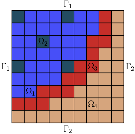
Our second example considers the construction of a surrogate model for a parametric neutron diffusion-reaction problem with spatially-varying coefficients and an external source. The goal is to construct a surrogate that can predict the average neutron flux for a given set of parameters. To this aim, we generate a dataset of 3,0003,000 samples, which we split into 2,6002,600 samples for training and 400400 for testing. Following [43], the computational domain Ω=(0,170)2\Omega=(0,170)^{2} is heterogeneous and consists of four different material regions, denoted by Ω1,…,Ω4\Omega_{1},\ldots,\Omega_{4} (see the left panel of Figure 2).

Refer to caption
Refer to caption
Refer to caption
Refer to caption
Refer to caption
Figure 2: Left: Computational domain used for the creation of the NDR dataset. Each subdomain is illustrated by a different color. Middle-Right: Example of samples contained in the NDR dataset.

The strong form of the problem is given as

∇⋅[D(x)∇ψ(x)]+α(x)∇ψ(x)\displaystyle\nabla\cdot[D(x)\nabla\psi(x)]+\alpha(x)\nabla\psi(x) =q⁡(x),\displaystyle=q(x),\qquad in​Ω,\displaystyle\text{in}\ \Omega,
ψ⁡(x)\displaystyle\psi(x) =0,\displaystyle=0, on​Γ1:=[0,170]×{1}∪{0}×[0,170],\displaystyle\text{on}\ \Gamma_{1}:=[0,170]\times\{1\}\cup\{0\}\times[0,170], (67)
D(x)∇ψ(x)⋅n(x)\displaystyle D(x)\nabla\psi(x)\cdot n(x) =0,\displaystyle=0, on​Γ2:=[0,170]×{0}∪{1}×[0,170],\displaystyle\text{on}\ \Gamma_{2}:=[0,170]\times\{0\}\cup\{1\}\times[0,170],

where xx denotes the spatial coordinates and ψ\psi is the neutron flux from Ω\Omega to IR. Functions D,α,qD,\alpha,q are defined as D⁡(x)=∑i=14𝟙Ωi​(x)​Di{D(x)=\sum_{i=1}^{4}\mathbbm{1}_{\Omega_{i}}(x)D_{i}}, q⁡(x)=∑i=13𝟙Ωi​(x)​qi{q(x)=\sum_{i=1}^{3}\mathbbm{1}_{\Omega_{i}}(x)q_{i}}, and α⁡(x)=∑i=14𝟙Ωi​(x)​αi{\alpha(x)=\sum_{i=1}^{4}\mathbbm{1}_{\Omega_{i}}(x)\alpha_{i}}, respectively (𝟙Ωi\mathbbm{1}_{\Omega_{i}} denotes the indicator function of the domain Ω\Omega). Problem (67) is then parametrized using 1111 parameters, which we sample from a uniform distribution U⁡(a,b)\pazocal{U}(a,b), specified by lower (a) and upper (b) bounds. More precisely, diffusion coefficients {Di}i=13\{D_{i}\}_{i=1}^{3} are sampled from U⁡(0.15,0.6)\pazocal{U}(0.15,0.6), while D4D_{4} is sampled from U⁡(0.2,0.8)\pazocal{U}(0.2,0.8). Reaction coefficients α1,…,α4\alpha_{1},\ldots,\alpha_{4} take on values from U⁡(0.0425,0.17)\pazocal{U}(0.0425,0.17), U⁡(0.065,0.26)\pazocal{U}(0.065,0.26), U⁡(0.04,0.16)\pazocal{U}(0.04,0.16), U⁡(0.005,0.02)\pazocal{U}(0.005,0.02), respectively. The values of sources {qi}i=13\{q_{i}\}_{i=1}^{3} are sampled from U⁡(5,20)\pazocal{U}(5,20), while the value value of q4q_{4} is set to 00. For each set of parameters/input features, we create a target cs=∫Ωψ⁡(x)​𝑑x/∫Ω𝑑xc_{s}=\int_{\Omega}\psi(x)\ dx/\int_{\Omega}dx by solving (67) numerically using the finite element method with a quadrilateral mesh (500500 elements in both spatial dimensions).

To build the desired surrogate, we train ResNet with dense residual blocks of width 1010, tanh activation function σ\sigma and parameters T=K=3T=K=3 and β1=β2=10−4\beta_{1}=\beta_{2}=10^{-4}. The identity hypothesis function and mean square loss functional are defined as 𝒽⁡(c^s,cs):=‖cs−c^s‖22{\mathcal{h}(\hat{c}_{s},c_{s}):=\|c_{s}-\hat{c}_{s}\|_{2}^{2}}.

As common for regression problems, we train ResNet using variants of the MOFFTR, ASTR1, SGD and ADAM methods with momentum. The details of how to handle the momentum in the multilevel framework can be found in [35, Appendix A]. The training is performed for a fixed computational budget, i.e., all solution strategies terminate as soon as C>Cmax{C>C_{\text{max}}}, where we set CmaxC_{\text{max}} to 2,0002,000.

Method Batch-size (batch-size/|D||\pazocal{D}|)
256 (25%) 1,024 (100%)
ftrain(×103){f_{\text{{train}}}(\times 10^{3})} fval(×103){f_{\text{{val}}}(\times 10^{3})} ftrain(×103){f_{\text{{train}}}(\times 10^{3})} fval(×103){f_{\text{{val}}}(\times 10^{3})}
SGD 0.61±0.300.61\pm 0.30 3.57±1.443.57\pm 1.44 1.87±1.321.87\pm 1.32 6.87±1.096.87\pm 1.09
ADAM 0.39±0.230.39\pm 0.23 5.77±0.795.77\pm 0.79 0.47±0.500.47\pm 0.50 5.35±0.235.35\pm 0.23
ASTR1 AdaGrad(μ=0.1\mu=0.1) 0.56±0.130.56\pm 0.13 5.41±0.725.41\pm 0.72 1.01±0.371.01\pm 0.37 5.72±1.185.72\pm 1.18
AdaGrad(μ=0.5\mu=0.5) 0.47±0.320.47\pm 0.32 4.62±2.714.62\pm 2.71 0.79±0.120.79\pm 0.12 7.04±4.937.04\pm 4.93
AdaGrad(μ=0.9\mu=0.9) 0.54±0.170.54\pm 0.17 7.43±2.487.43\pm 2.48 0.86±0.100.86\pm 0.10 4.93±2.564.93\pm 2.56
MAXGI 0.53±0.350.53\pm 0.35 5.67±1.235.67\pm 1.23 1.04±0.291.04\pm 0.29 4.98±1.284.98\pm 1.28
MOFFTR AdaGrad(μ=0.1\mu=0.1) 0.48±0.290.48\pm 0.29 0.89±0.310.89\pm 0.31 0.48±0.730.48\pm 0.73 1.02±0.421.02\pm 0.42
AdaGrad(μ=0.5\mu=0.5) 0.39±0.310.39\pm 0.31 0.95±0.290.95\pm 0.29 0.63±0.450.63\pm 0.45 1.29±0.531.29\pm 0.53
AdaGrad(μ=0.9\mu=0.9) 0.45±0.250.45\pm 0.25 1.06±0.361.06\pm 0.36 0.62±0.410.62\pm 0.41 1.36±0.491.36\pm 0.49
MAXGI 0.51±0.140.51\pm 0.14 0.91±0.300.91\pm 0.30 0.73±0.470.73\pm 0.47 1.38±0.451.38\pm 0.45
Table 2: NDR example: The mean and standard deviation of the value of train (ftrainf_{\text{train}}) and validation (fvalf_{\text{val}}) loss function achieved by training ResNet for 2,0002,000 epochs. The statistics is obtained from 1010 independent runs.
Figure 3: NDR example: The history of train (ftrainf_{\text{train}}) and validation (fvalf_{\text{val}}) loss function obtained while training ResNet for 2,0002,000 epochs with batch size 1,0241,024 (full dataset). The result with lowest fvalf_{\text{val}} among 1010 independent runs is reported.

We observe in Table 2 that all solution strategies, except SGD, achieve comparable values of the training loss (ftrainf_{\text{train}}). Interestingly, we also notice that all variants of the MOFFTR algorithm generalize better, i.e., reach a lower value of the validation loss (fvalf_{\text{val}}) than all single-level methods. This phenomenon can be also observed in Figure 3. The results presented in Table 2 suggest that the MOFFTR methods preserve good generalization properties in the presence of noise, a property of particular interest in surrogate modeling and other scientific applications that require reliable solutions.

5.2.3 Image classification using the SVNH dataset

Our last numerical example is associated with an image classification using SVNH dataset [42]. Each image is represented by 32×32{32\times 32} pixels and contains overlapping digits from 00 to 99. This dataset consists of 99,28999,289 samples, from which 73,25773,257 are used for training and 26,03226,032 for testing purposes. We pre-process all samples by standardizing the images, so that pixel values lie in the range [0,1][0,1], and by subtracting the mean from each pixel. In addition, we use standard data augmentation techniques, in particular image rotation, horizontal and vertical shift, and horizontal flip. The image classification is performed using ResNet with convolutional residual blocks (32 filters), ReLu activation function and parameters T=3T=3, K=5K=5, β1=10−3{\beta_{1}=10^{-3}}, β2=0.005{\beta_{2}=0.005}. Moreover, we use the softmax hypothesis function with the cross-entropy loss function.

The training of ResNets is performed using a batch size of 512512 and the same stopping criterion as that used for the Indian Pines example in Section 5.2.1. For this experiment, we consider the MOFFTR, ASTR1 and SGD methods without momentum. Table 3 reports the computational cost and validation accuracy achieved by all methods. The study is performed with respect to an increasing number of refinement levels**** ** The number of levels utilized by the MOFFTR algorithms increases linearly with refinement level..

Figure 4: SVNH example: The validation accuracy as a function of total computational cost obtained while training ResNet with 1717 residual block (three refinement levels). The run with the highest validation accuracy is selected among 1010 independent runs.
Method Levels (residual blocks)
2 (9) 3 (17) 4 (33)
C{C} accval\text{{acc}}_{\text{{val}}} C{C} accval\text{{acc}}_{\text{{val}}} C{C} accval\text{{acc}}_{\text{{val}}}
SGD 280 92.4% 313 92.7% 336 92.9%
ASTR1 AdaGrad(μ=0.1\mu=0.1) 325 92.4% 361361 92.6% 341 92.8%
AdaGrad(μ=0.5\mu=0.5) 334 92.3% 333333 92.4% 328 92.7%
AdaGrad(μ=0.9\mu=0.9) 351 92.1% 358358 92.4% 369 92.6%
MAXGI 313 92.3% 317317 92.7% 325 92.8%
MOFFTR AdaGrad(μ=0.1\mu=0.1) 134 92.3% 105105 92.7% 139 92.9%
AdaGrad(μ=0.5\mu=0.5) 148 92.2% 135135 92.6% 144 92.8%
AdaGrad(μ=0.9\mu=0.9) 169 92.1% 171171 92.6% 151 92.8%
MAXGI 158 92.5% 146146 92.9% 143 93.1%
Table 3: SVNH example: The total computational cost CC and validation accuracy accval\text{acc}_{\text{val}}, which were required to train ResNet with increasing depth (refinement level). The best result in terms of validation accuracy is reported among 1010 independent runs.

These results suggest that increasing the network depth enhances its representation capacity, which in turn justifies a higher computational cost. We also notice that all variants of the MOFFTR method require lower computational cost than single-level solution strategies while achieving comparable accuracy. The obtained computational gains vary from the factor of 1.71.7 to 3.43.4. This can be observed independently of the refinement level, which indicates that the MOFFTR algorithm has a clear potential to speed up the training of large-scale networks, such as the ones used in real-life applications. We also note that, among all variants of the MOFFTR framework, the choice of the MAXGI weights yields higher validation accuracy than that obtained with the AdaGrad-like variants. We finally observe that, among all AdaGrad-like variants, the configuration with μ=0.1\mu=0.1 achieves the highest validation accuracy as well as the lowest computational cost. The fact that a similar observation can be made also for the corresponding single-level ASTR1 methods suggests that exploring values of μ\mu other than the traditional μ=0.5\mu=0.5 might be beneficial in practice.

6 Conclusion

We have presented a class of multilevel algorithms for unconstrained minimization which do not require the computation of the objective function’s value. We have also shown that the performance of algorithms of the class is competitive in the presence of noise-induced by subsampling in the context of deep neural network training. The convergence theory of two interesting subclasses has been analyzed and shown to match the state of the art. Our experiments also indicate that, although currently not covered by our theory, the benefits of the multilevel approach are preserved when momentum is added to the framework. The authors are well aware that only continued experimentation will reveal the true practical value of the present proposal, but they note that the first numerical tests are encouraging.

Acknowledgements

A. Kopaničáková gratefully acknowledges support of the Swiss National Science Foundation through the project ”Multilevel training of DeepONets — multiscale and multiphysics applications” (grant no. 206745), and partial support of Platform for Advanced Scientific Computing (PASC) under the project EXATRAIN. Ph. L. Toint acknowledges the continued and friendly partial support of ANITI.

References

  • [1] N. M. Alexandrov and R. L. Lewis. An overview of first-order model management for engineering optimization. Optimization and Engineering, 2:413–430, 2001.
  • [2] M. F. Baumgardner, L. L. Biehl, and D. A. Landgrebe. 220 band AVIRIS Hyperspectral Image Data Set: June 12, 1992 Indian Pine TeSite 3. Purdue University Research Repository, 10(7):991, 2015.
  • [3] A. Beck and N. Hallak. Optimization problems involving group sparsity terms. Mathematical Programming, 2018. online.
  • [4] A. Borzi and K. Kunisch. A globalisation strategy for the multigrid solution of elliptic optimal control problems. Optimization Methods and Software, 21(3):445–459, 2006.
  • [5] A. Bouaricha and R. B. Schnabel. Tensor methods for large sparse systems of nonlinear equations. Mathematical Programming, 82(3):377–412, 1998.
  • [6] W. L. Briggs, V. E. Henson, and S. F. McCormick. A Multigrid Tutorial. SIAM, Philadelphia, USA, 2nd edition, 2000.
  • [7] C. Cartis, N. I. M. Gould, and Ph. L. Toint. Evaluation complexity of algorithms for nonconvex optimization. Number 30 in MOS-SIAM Series on Optimization. SIAM, Philadelphia, USA, June 2022.
  • [8] B. Chang, L. Meng, E. Haber, F. Tung, and D. Begert. Multi-level residual networks from dynamical systems view. arXiv:1710.10348, 2017.
  • [9] I. Chatzigeorgiou. Bounds on the Lambert function and their application to the outage analysis of user cooperation. IEEE Communications Letters, 17(8):1505–1508, 2013.
  • [10] A. R. Conn, N. I. M. Gould, and Ph. L. Toint. LANCELOT: a Fortran package for large-scale nonlinear optimization (Release A). Number 17 in Springer Series in Computational Mathematics. Springer Verlag, Heidelberg, Berlin, New York, 1992.
  • [11] A. R. Conn, N. I. M. Gould, and Ph. L. Toint. Trust-Region Methods. Number 1 in MOS-SIAM Optimization Series. SIAM, Philadelphia, USA, 2000.
  • [12] R. M. Corless, G. H. Gonnet, D. E. Hare, D. J. Jeffrey, and D. E. Knuth. On the Lambert W function. Advances in Computational Mathematics, 5:329––359, 1996.
  • [13] E. C. Cyr, S. Günther, and J. B. Schroder. Multilevel initialization for layer-parallel deep neural network training. International Journal of Computing and Visualization in Science and Engineering, 2021.
  • [14] J. Duchi, E. Hazan, and Y. Singer. Adaptive subgradient methods for online learning and stochastic optimization. Journal of Machine Learning Research, 12, July 2011.
  • [15] F. Chollet et al. Keras, 2015. https://keras.io.
  • [16] M. Fisher. Minimization algorithms for variational data assimilation. In Recent Developments in Numerical Methods for Atmospheric Modelling, pages 364–385, Reading, UK, 1998. European Center for Medium-Range Weather Forecasts.
  • [17] K. Fujisawa, M. Kojima, and K. Nakata. Exploiting sparsity in primal-dual interior-point methods for semidefinite programming. Mathematical Programming, Series B, 79(1–3):235–253, 1997.
  • [18] L. Gaedke-Merzhäuser, A. Kopaničáková, and R. Krause. Multilevel minimization for deep residual networks. In ESAIM. Proceedings and Surveys. 71:131-144, 2021.
  • [19] D. M. Gay. Automatically finding and exploiting partially separable structure in nonlinear programming problems. Technical report, Bell Laboratories, Murray Hill, New Jersey, USA, 1996.
  • [20] E. Gelman and J. Mandel. On multilevel iterative methods for optimization problems. Mathematical Programming, 48(1):1–17, 1990.
  • [21] D. Goldfarb and S. Wang. Partial-update Newton methods for unary, factorable and partially separable optimization. SIAM Journal on Optimization, 3(2):383–397, 1993.
  • [22] S. Gratton, S. Jerad, and Ph. L. Toint. Convergence properties of an objective-function-free optimization regularization algorithm, including an 𝒪(ϵ−3/2)\mathcal{O}(\epsilon^{-3/2}) complexity bound. arXiv:2203.09947, 2022.
  • [23] S. Gratton, S. Jerad, and Ph. L. Toint. First-order objective-function-free optimization algorithms and their complexity. arXiv:2203.01757, 2022.
  • [24] S. Gratton, S. Jerad, and Ph. L. Toint. Parametric complexity analysis for a class of first-order Adagrad-like algorithms. arXiv:2203.01647, 2022.
  • [25] S. Gratton, M. Mouffe, A. Sartenaer, Ph. L. Toint, and D. Tomanos. Numerical experience with a recursive trust-region method for multilevel nonlinear bound-constrained optimization. Optimization Methods and Software, 25(3):359 – 386, 2010.
  • [26] S. Gratton, A. Sartenaer, and Ph. L. Toint. Recursive trust-region methods for multiscale nonlinear optimization. SIAM Journal on Optimization, 19(1):414–444, 2008.
  • [27] S. Gratton and Ph. L. Toint. Approximate invariant subspaces and quasi-Newton optimization methods. Optimization Methods and Software, 25(4):507–529, 2010.
  • [28] A. Griewank and Ph. L. Toint. On the unconstrained optimization of partially separable functions. In M. J. D. Powell, editor, Nonlinear Optimization 1981, pages 301–312, London, 1982. Academic Press.
  • [29] E. Haber and L. Ruthotto. Stable architectures for deep neural networks. Inverse Problems, 34(1):014004, 2017.
  • [30] E. Haber, L. Ruthotto, E. Holtham, and S.-H. Jun. Learning across scales—multiscale methods for convolution neural networks. In Thirty-Second AAAI Conference on Artificial Intelligence, 2018.
  • [31] K. He, X. Zhang, S. Ren, and J. Sun. Identity mappings in deep residual networks. In European conference on computer vision, pages 630–645, Heidelberg, Berlin, New York, 2016. Springer Verlag.
  • [32] S. Ioffe and Ch. Szegedy. Batch normalization: Accelerating deep network training by reducing internal covariate shift. arXiv:1502.03167, 2015.
  • [33] D. Kingma and J. Ba. Adam: A method for stochastic optimization. In Proceedings in the International Conference on Learning Representations (ICLR), 2015.
  • [34] A. Kopaničáková. On the use of hybrid coarse-level models in multilevel minimization methods. arXiv:2211.15078, 2022.
  • [35] A. Kopaničáková and R. Krause. Globally convergent multilevel training of deep residual networks. SIAM Journal on Scientific Computing, 0:S254–S280, 2022.
  • [36] R. Kornhuber. Adaptive monotone multigrid methods for some non-smooth optimization problems. In R. Glowinski, J. Périaux, Z. Shi, and O. Widlund, editors, Domain Decomposition Methods in Sciences and Engineering, pages 177–191. J. Wiley and Sons, Chichester, England, 1997.
  • [37] J. B. Lasserre. Convergent semidefinite relaxation in polynomial optimization with sparsity. Technical report, LAAS-CNRS, 7, avenue du Colonel Roche, 31077 Toulouse, France, November 2005.
  • [38] M. Lewis and S. G. Nash. Practical aspects of multiscale optimization methods for VLSICAD. In Jason Cong and Joseph R. Shinnerl, editors, Multiscale Optimization and VLSI/CAD, pages 265–291, Dordrecht, The Netherlands, 2002. Kluwer Academic Publishers.
  • [39] M. Lewis and S. G. Nash. Model problems for the multigrid optimization of systems governed by differential equations. SIAM Journal on Scientific Computing, 26(6):1811–1837, 2005.
  • [40] J. Mareček, P. Richtárik, and M. Takáč. Distributed block coordinate descent for minimizing partially separable functions. Technical report, Department of Mathematics and Statistics, University of Edinburgh, Edinburgh, Scotland, 2014.
  • [41] S. G. Nash. A multigrid approach to discretized optimization problems. Optimization Methods and Software, 14:99–116, 2000.
  • [42] Y. Netzer, T. Wang, A. Coates, A. Bissacco, B. Wu, and A.Y. Ng. Reading digits in natural images with unsupervised feature learning, 2011.
  • [43] Z. M. Prince and J. C. Ragusa. Parametric uncertainty quantification using proper generalized decomposition applied to neutron diffusion. International Journal for Numerical Methods in Engineering, 119(9):899–921, 2019.
  • [44] A. F. Queiruga, N. B. Erichson, D. Taylor, and M. W. Mahoney. Continuous-in-depth neural networks. arXiv:2008.02389, 2020.
  • [45] S. Reddi, S. Kale, and S. Kumar. On the convergence of Adam and beyond. In Proceedings in the International Conference on Learning Representations (ICLR), 2018.
  • [46] H. Robbins and S. Monro. A stochastic approximation method. The Annals of Mathematical Statistics, 22(3):400––407, 1951.
  • [47] T. Tieleman and G. Hinton. Lecture 6.5-RMSPROP. COURSERA: Neural Networks for Machine Learning, 2012.
  • [48] Ph. L. Toint. A note on sparsity exploiting quasi-Newton methods. Mathematical Programming, 21(2):172–181, 1981.
  • [49] Ph. L. Toint. Towards an efficient sparsity exploiting Newton method for minimization. In I. S. Duff, editor, Sparse Matrices and Their Uses, pages 57–88, London, 1981. Academic Press.
  • [50] E. Weinan. A proposal on machine learning via dynamical systems. Communications in Mathematics and Statistics, 5(1):1–11, 2017.
  • [51] Y. Yuan. Recent advances in trust region algorithms. Mathematical Programming, Series A, 151(1):249–281, 2015.
  • [52] D. Zhou, J. Chen, Y. Tang, Z. Yang, Y. Cao, and Q. Gu. On the convergence of adaptive gradient methods for nonconvex optimization. arXiv:2080.05671, 2020.

Appendix A Proof of Theorem 3.8

We first recall a useful technical result.

Lemma A.1
[23, Lemma 3.5] Consider and arbitrary i∈{1,…,n}i\in\{1,\ldots,n\} and suppose that there exists a jςj_{\varsigma} such that min⁡[gi,j2ςi,gi,j2vi,j]≤ςi​ for ​j≥jς.\min\left[\frac{g_{i,j}^{2}}{\varsigma_{i}},\frac{g_{i,j}^{2}}{v_{i,j}}\right]\leq\varsigma_{i}\;\;\mbox{ for }\;\;j\geq j_{\varsigma}. (68) Then min⁡[gi,j2ςi,gi,j2vi,j]≥gi,j22​ςi​ for ​j≥jς.\min\left[\frac{g_{i,j}^{2}}{\varsigma_{i}},\frac{g_{i,j}^{2}}{v_{i,j}}\right]\geq\frac{g_{i,j}^{2}}{2\varsigma_{i}}\;\;\mbox{ for }\;\;j\geq j_{\varsigma}. (69)

Proof of Theorem 3.8

We obtain from (43) and (6) that, for i≥iϑi\geq i_{\vartheta},

f⁡(xr,iϑ)−f⁡(xr,i+1)≥12​∑k=iϑ+1i∑j=1ngr,k,j2wr,k,j​[β1,r−β2,r+12​α2​Lwℓ,k,j].f(x_{r,i_{\vartheta}})-f(x_{r,i+1})\geq\frac{1}{2}\sum_{k=i_{\vartheta}+1}^{i}\sum_{j=1}^{n}\frac{g_{r,k,j}^{2}}{w_{r,k,j}}\left[\beta_{1,r}-\frac{\beta_{2,r}+{\scriptstyle\frac{1}{2}}\alpha^{2}L}{w_{\ell,k,j}}\right].

Moreover, (45) and (52) also ensure that, since i≥iϑi\geq i_{\vartheta},

β1,r−β2,r+12​α2​Lwℓ,k,j≥ϑ\beta_{1,r}-\frac{\beta_{2,r}+{\scriptstyle\frac{1}{2}}\alpha^{2}L}{w_{\ell,k,j}}\geq\vartheta

for all j∈{1,…,n}j\in\{1,\ldots,n\}, so that

f⁡(xr,iϑ+1)−f⁡(xr,i+1)\displaystyle f(x_{r,i_{\vartheta}}+1)-f(x_{r,i+1}) ≥ϑ2​∑k=iϑ+1i∑j=1ngr,k,j2wr,k,j\displaystyle\geq\frac{\vartheta}{2}\sum_{k=i_{\vartheta}+1}^{i}\sum_{j=1}^{n}\frac{g_{r,k,j}^{2}}{w_{r,k,j}}
≥ϑ2​∑k=iϑ+1i∑j=1ngr,k,j2max⁡[ςj,vr,k]​(k+1)μ\displaystyle\geq\frac{\vartheta}{2}\sum_{k=i_{\vartheta}+1}^{i}\sum_{j=1}^{n}\frac{g_{r,k,j}^{2}}{\max[\varsigma_{j},v_{r,k}](k+1)^{\mu}}
≥ϑ2​(i+1)μ​∑k=iϑ+1i∑j=1nmin⁡[gr,k,j2ςj,gr,k,j2vr,k]\displaystyle\geq\frac{\vartheta}{2(i+1)^{\mu}}\sum_{k=i_{\vartheta}+1}^{i}\sum_{j=1}^{n}\min\left[\frac{g_{r,k,j}^{2}}{\varsigma_{j}},\frac{g_{r,k,j}^{2}}{v_{r,k}}\right]
≥ϑ⁡(i−iϑ)2​(i+1)μ​mink∈{iϑ,…,i}⁡(∑j=1nmin⁡[gr,k,j2ςj,gr,k,j2vr,k]).\displaystyle\geq\frac{\vartheta(i-i_{\vartheta})}{2(i+1)^{\mu}}\min_{k\in\{i_{\vartheta},\ldots,i\}}\left(\sum_{j=1}^{n}\min\left[\frac{g_{r,k,j}^{2}}{\varsigma_{j}},\frac{g_{r,k,j}^{2}}{v_{r,k}}\right]\right).

But, using (50) in Lemma 3.7,

f(x0)−f(xiϑ+1)=f(xr,0)−f(xiϑ+1)≥−n(β2,r+12α2L)∑k=0iϑa(k)2.f(x_{0})-f(x_{i_{\vartheta}+1})=f(x_{r,0})-f(x_{i_{\vartheta}+1})\geq-n(\beta_{2,r}+{\scriptstyle\frac{1}{2}}\alpha^{2}L)\sum_{k=0}^{i_{\vartheta}}a(k)^{2}. (70)

Combining these two last inequalities with AS.3 then gives that

mink∈{iϑ,…,i}⁡(∑j=1nmin⁡[gr,k,j2ςj,gr,k,j2vr,k])\displaystyle\min_{k\in\{i_{\vartheta},\ldots,i\}}\left(\sum_{j=1}^{n}\min\left[\frac{g_{r,k,j}^{2}}{\varsigma_{j}},\frac{g_{r,k,j}^{2}}{v_{r,k}}\right]\right) ≤2​(i+1)μϑ⁡(i−iϑ)​(f⁡(xiϑ+1)−f⁡(xi+1))\displaystyle\leq\frac{2(i+1)^{\mu}}{\vartheta(i-i_{\vartheta})}\Big(f(x_{i_{\vartheta}+1})-f(x_{i+1})\Big)
=2​(i+1)μϑ⁡(i−iϑ)​(f⁡(x0)−f⁡(xi+1)+f⁡(xiϑ+1)−f⁡(x0))\displaystyle=\frac{2(i+1)^{\mu}}{\vartheta(i-i_{\vartheta})}\Big(f(x_{0})-f(x_{i+1})+f(x_{i_{\vartheta}+1})-f(x_{0})\Big)
≤2​(i+1)μϑ⁡(i−iϑ)​(Γ0+n⁡(β2,r+12​α2​L)​∑k=0iϑa​(k)2)\displaystyle\leq\frac{2(i+1)^{\mu}}{\vartheta(i-i_{\vartheta})}\Big(\Gamma_{0}+n(\beta_{2,r}+{\scriptstyle\frac{1}{2}}\alpha^{2}L)\sum_{k=0}^{i_{\vartheta}}a(k)^{2}\Big)

from which we obtain that there exists a subsequence {it}⊆{i}iϑ∞\{i_{t}\}\subseteq\{i\}_{i_{\vartheta}}^{\infty} such that

∑j=1nmin⁡[gr,it,j2ςj,gr,it,j2vr,it]≤2​(it+1)μϑ⁡(it−iϑ)​[Γ0+n⁡(β2,r+12​α2​L)​∑k=0iϑa​(k)2].\sum_{j=1}^{n}\min\left[\frac{g_{r,i_{t},j}^{2}}{\varsigma_{j}},\frac{g_{r,i_{t},j}^{2}}{v_{r,i_{t}}}\right]\leq\frac{2(i_{t}+1)^{\mu}}{\vartheta(i_{t}-i_{\vartheta})}\left[\Gamma_{0}+n(\beta_{2,r}+{\scriptstyle\frac{1}{2}}\alpha^{2}L)\sum_{k=0}^{i_{\vartheta}}a(k)^{2}\right]. (71)

Now,

(it+1)μit−iϑ<2μ​itμit−iϑ<2​itμit−iϑ=2​itμ​it(it−iϑ)​it=itit−iϑ⋅2it1−μ≤2​(iϑ+1)it1−μ,\frac{(i_{t}+1)^{\mu}}{i_{t}-i_{\vartheta}}<\frac{2^{\mu}i_{t}^{\mu}}{i_{t}-i_{\vartheta}}<\frac{2i_{t}^{\mu}}{i_{t}-i_{\vartheta}}=\frac{2i_{t}^{\mu}i_{t}}{(i_{t}-i_{\vartheta})i_{t}}=\frac{i_{t}}{i_{t}-i_{\vartheta}}\cdot\frac{2}{i_{t}^{1-\mu}}\leq\frac{2(i_{\vartheta}+1)}{i_{t}^{1-\mu}}, (72)

where we used the facts that μ<1\mu<1 and that itit−iϑ\frac{i_{t}}{i_{t}-i_{\vartheta}} is a decreasing function for it≥iϑ+1i_{t}\geq i_{\vartheta}+1. As a consequence, we obtain from (71) that

∑j=1nmin⁡[gr,it,j2ςj,gr,it,j2vr,it]≤4​(iϑ+1)ϑ​it1−μ​[Γ0+n⁡(β2,r+12​α2​L)​∑k=0iϑa​(k)2].\sum_{j=1}^{n}\min\left[\frac{g_{r,i_{t},j}^{2}}{\varsigma_{j}},\frac{g_{r,i_{t},j}^{2}}{v_{r,i_{t}}}\right]\leq\frac{4(i_{\vartheta}+1)}{\vartheta i_{t}^{1-\mu}}\left[\Gamma_{0}+n(\beta_{2,r}+{\scriptstyle\frac{1}{2}}\alpha^{2}L)\sum_{k=0}^{i_{\vartheta}}a(k)^{2}\right].

If we now define

iς=def(4​(iϑ+1)​[Γ0+12​n​(β2,r+12​α2​L)​∑k=0iϑa​(k)2]ϑ​ςmin)11−μ,i_{\varsigma}\stackrel{{\scriptstyle\rm def}}{{=}}\left(\frac{4(i_{\vartheta}+1)\left[\Gamma_{0}+{\scriptstyle\frac{1}{2}}n(\beta_{2,r}+{\scriptstyle\frac{1}{2}}\alpha^{2}L)\sum_{k=0}^{i_{\vartheta}}a(k)^{2}\right]}{\vartheta\varsigma_{\min}}\right)^{\frac{1}{1-\mu}},

we see that, for all it≥iςi_{t}\geq i_{\varsigma},

min⁡[gr,it,j2ςj,gr,it,j2vr,it]≤ςmin.\min\left[\frac{g_{r,i_{t},j}^{2}}{\varsigma_{j}},\frac{g_{r,i_{t},j}^{2}}{v_{r,i_{t}}}\right]\leq\varsigma_{\min}.

We then apply Lemma A.1 to deduce from (71) that, for all it≥iςi_{t}\geq i_{\varsigma},

∑j=1ngr,it,j22​ςj≤2​(it+1)μϑ⁡(it−iϑ)​[Γ0+n⁡(β2,r+12​α2​L)​∑k=0iϑa​(k)2]\sum_{j=1}^{n}\frac{g_{r,i_{t},j}^{2}}{2\varsigma_{j}}\leq\frac{2(i_{t}+1)^{\mu}}{\vartheta(i_{t}-i_{\vartheta})}\left[\Gamma_{0}+n(\beta_{2,r}+{\scriptstyle\frac{1}{2}}\alpha^{2}L)\sum_{k=0}^{i_{\vartheta}}a(k)^{2}\right]

and therefore, because ςj≤1\varsigma_{j}\leq 1, that

‖gr,it‖2≤(it+1)μit−iϑ​(2ϑ)​[Γ0+n⁡(β2,r+12​α2​L)​∑k=0iϑa​(k)2]\|g_{r,i_{t}}\|^{2}\ \leq\frac{(i_{t}+1)^{\mu}}{i_{t}-i_{\vartheta}}\left(\frac{2}{\vartheta}\right)\left[\Gamma_{0}+n(\beta_{2,r}+{\scriptstyle\frac{1}{2}}\alpha^{2}L)\sum_{k=0}^{i_{\vartheta}}a(k)^{2}\right]

for all it≥iςi_{t}\geq i_{\varsigma}. This then gives (51), the last inequality following from (72) and (6). □\Box

Appendix B Proof of Theorem 3.9

Again, we first recall a useful technical lemma.

Lemma B.1
[23, Lemma 3.1] Let {ak}k≥0\{a_{k}\}_{k\geq 0} be a non-negative sequence, α>0\alpha>0, ξ>0\xi>0 and define, for each k≥0k\geq 0, bk=∑t=0katb_{k}=\sum_{t=0}^{k}a_{t}. Then ∑k=0iak(ξ+bk)α≤{1(1−α)​((ξ+bi)1−α−ξ1−α)if ​α≠1,log⁡(ξ+biξ)if ​α=1.\sum_{k=0}^{i}\frac{a_{k}}{(\xi+b_{k})^{\alpha}}\leq\left\{\begin{array}[]{ll}\frac{\displaystyle 1}{\displaystyle(1-\alpha)}((\xi+b_{i})^{1-\alpha}-\xi^{1-\alpha})&\;\;\mbox{if }\;\;\alpha\neq 1,\\[8.61108pt] \log\left(\frac{\displaystyle\xi+b_{i}}{\displaystyle\xi}\right)&\;\;\mbox{if }\;\;\alpha=1.\end{array}\right. (73)

Proof of Theorem 3.9

We first note that (54) implies that

ςμ≤maxj∈{1,…,n}⁡wr,i,j≤(ς+∑k=0i‖gr,k‖2)μ\varsigma^{\mu}\leq\max_{j\in\{1,\ldots,n\}}w_{r,i,j}\leq\left(\varsigma+\sum_{k=0}^{i}\|g_{r,k}\|^{2}\right)^{\mu} (74)

for all i≥0i\geq 0. We also deduce from (6) and (43) in Lemma 3.6 with ℓ=r\ell=r that, for i≥0i\geq 0,

f⁡(xi+1)≤f⁡(x0)−β1,r​∑k=0i‖gr,k‖2maxj∈{1,…,n}⁡wr,k,j+(β2,r+12​L)​∑j=1n∑k=0igr,k,j2wr,k,j2.f(x_{i+1})\leq f(x_{0})-\beta_{1,r}\sum_{k=0}^{i}\frac{\displaystyle\|g_{r,k}\|^{2}}{\displaystyle\max_{j\in\{1,\ldots,n\}}w_{r,k,j}}+\left(\beta_{2,r}+{\scriptstyle\frac{1}{2}}L\right)\displaystyle\sum_{j=1}^{n}\displaystyle\sum_{k=0}^{i}\frac{g_{r,k,j}^{2}}{w_{r,k,j}^{2}}. (75)
Case (i).

Suppose first that μ∈(0,12)\mu\in(0,{\scriptstyle\frac{1}{2}}). For each j∈{1,…,n}j\in\{1,\ldots,n\}, we then apply (73) in Lemma B.1 with ak=gr,k,j2a_{k}=g_{r,k,j}^{2}, ξ=ς\xi=\varsigma and α=2​μ<1\alpha=2\mu<1, and obtain from (13) and (54) that,

∑k=0igr,k,j2wr,k,j2≤11−2​μ​[(ς+∑k=0igr,k,j2)1−2​μ−ς1−2​μ]≤11−2​μ​(ς+∑k=0igr,k,j2)1−2​μ.\displaystyle\sum_{k=0}^{i}\frac{g_{r,k,j}^{2}}{w_{r,k,j}^{2}}\leq\frac{\displaystyle 1}{\displaystyle 1-2\mu}\left[\left(\varsigma+\displaystyle\sum_{k=0}^{i}g_{r,k,j}^{2}\right)^{1-2\mu}-\varsigma^{1-2\mu}\right]\leq\frac{\displaystyle 1}{\displaystyle 1-2\mu}\left(\varsigma+\displaystyle\sum_{k=0}^{i}g_{r,k,j}^{2}\right)^{1-2\mu}. (76)

Now substituting this bound in (75) and using AS.3 gives that

β1,r​∑k=0i‖gr,k‖2maxj∈{1,…,n}⁡wr,k,j≤Γ0+n⁡(β2,r+12​L)1−2​μ​(ς+∑k=0i‖gr,k‖2)1−2​μ.\beta_{1,r}\sum_{k=0}^{i}\frac{\displaystyle\|g_{r,k}\|^{2}}{\displaystyle\max_{j\in\{1,\ldots,n\}}w_{r,k,j}}\leq\Gamma_{0}+\frac{n(\beta_{2,r}+{\scriptstyle\frac{1}{2}}L)}{1-2\mu}\left(\varsigma+\sum_{k=0}^{i}\|g_{r,k}\|^{2}\right)^{1-2\mu}. (77)

Suppose now that

∑k=0i‖gr,k‖2≥max⁡{ς,12​[(1−2​μ)​Γ0n⁡(β2,r+12​L)]11−2​μ},\sum_{k=0}^{i}\|g_{r,k}\|^{2}\geq\max\left\{\varsigma,\frac{1}{2}\left[\frac{(1-2\mu)\Gamma_{0}}{n(\beta_{2,r}+{\scriptstyle\frac{1}{2}}L)}\right]^{{\scriptstyle\frac{1}{1-2\mu}}}\right\}, (78)

implying

ς+∑k=0i‖gr,k‖2≤2​∑k=0i‖gr,k‖2​and​Γ0≤n⁡(β2,r+12​L)1−2​μ​(2​∑k=0i‖gr,k‖2)1−2​μ.\varsigma+\sum_{k=0}^{i}\|g_{r,k}\|^{2}\leq 2\sum_{k=0}^{i}\|g_{r,k}\|^{2}\;\;\mbox{and}\;\;\Gamma_{0}\leq\frac{n(\beta_{2,r}+{\scriptstyle\frac{1}{2}}L)}{1-2\mu}\left(2\sum_{k=0}^{i}\|g_{r,k}\|^{2}\right)^{1-2\mu}.

Then, using (77) and (74),

β1,r2μ​[∑k=0i‖gr,k‖2]μ​∑k=0i‖gr,k‖2≤22​(1−μ)​n​(β2,r+12​L)1−2​μ​(∑k=0i‖gr,k‖2)1−2​μ.\frac{\beta_{1,r}}{2^{\mu}\left[\sum_{k=0}^{i}\|g_{r,k}\|^{2}\right]^{\mu}}\sum_{k=0}^{i}\|g_{r,k}\|^{2}\leq\frac{2^{2(1-\mu)}n(\beta_{2,r}+{\scriptstyle\frac{1}{2}}L)}{1-2\mu}\left(\sum_{k=0}^{i}\|g_{r,k}\|^{2}\right)^{1-2\mu}.

Solving this inequality for ∑k=0i‖gr,k‖2\sum_{k=0}^{i}\|g_{r,k}\|^{2} and using the fact that 22​(1−μ)<42^{2(1-\mu)}<4 gives that

∑k=0i‖gr,k‖2<[4​n​(β2,r+12​L)β1,r​(1−2​μ)]1μ\sum_{k=0}^{i}\|g_{r,k}\|^{2}<\left[\frac{4n(\beta_{2,r}+{\scriptstyle\frac{1}{2}}L)}{\beta_{1,r}(1-2\mu)}\right]^{{\scriptstyle\frac{1}{\mu}}}

and therefore

averagek∈{0,…,i}‖gr,k‖2<[4​n​(β2,r+12​L)β1,r​(1−2​μ)]1μ⋅1i+1.\average_{k\in\{0,\ldots,i\}}\|g_{r,k}\|^{2}<\left[\frac{4n(\beta_{2,r}+{\scriptstyle\frac{1}{2}}L)}{\beta_{1,r}(1-2\mu)}\right]^{{\scriptstyle\frac{1}{\mu}}}\cdot\frac{1}{{i+1}}. (79)

Alternatively, if (78) fails, then

averagek∈{0,…,i}‖gr,k‖2<max⁡{ς,12​[(1−2​μ)​Γ0n⁡(β2,r+12​L)]11−2​μ}⋅1i+1.\average_{k\in\{0,\ldots,i\}}\|g_{r,k}\|^{2}<\max\left\{\varsigma,\frac{1}{2}\left[\frac{(1-2\mu)\Gamma_{0}}{n(\beta_{2,r}+{\scriptstyle\frac{1}{2}}L)}\right]^{{\scriptstyle\frac{1}{1-2\mu}}}\right\}\cdot\frac{1}{i+1}. (80)

Combining (79), (80) and (6) gives (57) for 0<μ<120<\mu<{\scriptstyle\frac{1}{2}}.

Case (ii).

Let us now consider the case where μ=12\mu={\scriptstyle\frac{1}{2}}. For each j∈{1,…,n}j\in\{1,\ldots,n\}, we apply (73) in Lemma B.1 with ak=gr,k,j2a_{k}=g_{r,k,j}^{2}, ξ=ς\xi=\varsigma and α=2​μ=1\alpha=2\mu=1 and obtain that,

∑j=1n∑k=0igr,k,j2wr,k,j2≤∑j=1nlog⁡(1ς​(ς+∑k=0igr,k,j2))≤n​log⁡(1+1ς​∑k=0i‖gr,k‖2)\displaystyle\sum_{j=1}^{n}\displaystyle\sum_{k=0}^{i}\frac{g_{r,k,j}^{2}}{w_{r,k,j}^{2}}\leq\displaystyle\sum_{j=1}^{n}\log\left(\frac{1}{\varsigma}\left(\varsigma+\displaystyle\sum_{k=0}^{i}g_{r,k,j}^{2}\right)\right)\leq n\log\left(1+\frac{1}{\varsigma}\displaystyle\sum_{k=0}^{i}\|g_{r,k}\|^{2}\right)

and substituting this bound in (75) then gives that

β1,r​∑k=0i‖gr,k‖2maxj∈{1,…,n}⁡wr,k,j≤Γ0+12​n​(β2,r+12​L)​log⁡(1+1ς​∑k=0i‖gr,k‖2).\beta_{1,r}\sum_{k=0}^{i}\frac{\displaystyle\|g_{r,k}\|^{2}}{\displaystyle\max_{j\in\{1,\ldots,n\}}w_{r,k,j}}\leq\Gamma_{0}+{\scriptstyle\frac{1}{2}}n(\beta_{2,r}+{\scriptstyle\frac{1}{2}}L)\log\left(1+\frac{1}{\varsigma}\displaystyle\sum_{k=0}^{i}\|g_{r,k}\|^{2}\right).

Suppose now that

∑k=0i‖gr,k‖2≥max⁡[ς,e2​Γ0n⁡(β2,r+12​L)],\sum_{k=0}^{i}\|g_{r,k}\|^{2}\geq\max\left[\varsigma,e^{\frac{2\Gamma_{0}}{n(\beta_{2,r}+{\scriptstyle\frac{1}{2}}L)}}\right], (81)

implying that

ς+∑k=0i‖gr,k‖2≤2​∑k=0i‖gr,k‖2​and​Γ0≤12​n​(βr,2+12​L)​log⁡(2ς​∑k=0i‖gr,k‖2).\varsigma+\sum_{k=0}^{i}\|g_{r,k}\|^{2}\leq 2\sum_{k=0}^{i}\|g_{r,k}\|^{2}\;\;\mbox{and}\;\;\Gamma_{0}\leq{\scriptstyle\frac{1}{2}}n(\beta_{r,2}+{\scriptstyle\frac{1}{2}}L)\log\left(\frac{2}{\varsigma}\displaystyle\sum_{k=0}^{i}\|g_{r,k}\|^{2}\right).

Using (74) for μ=12\mu={\scriptstyle\frac{1}{2}}, we obtain then that

β1,r2​∑k=0i‖gr,k‖2​∑k=0i‖gr,k‖2≤n⁡(βr,k+12​L)\frac{\displaystyle\beta_{1,r}}{\displaystyle\sqrt{2}\,\sqrt{\sum_{k=0}^{i}\|g_{r,k}\|^{2}}}\displaystyle\sum_{k=0}^{i}\|g_{r,k}\|^{2}\leq n(\beta_{r,k}+{\scriptstyle\frac{1}{2}}L)\vskip-5.69054pt

and thus that

βr,1​∑k=0i‖gr,k‖2≤2​2​max⁡[3​βr,1,n⁡(βr,2+12​L)]​log⁡(2ς​∑k=0i‖gr,k‖2).\beta_{r,1}\sqrt{\displaystyle\sum_{k=0}^{i}\|g_{r,k}\|^{2}}\leq 2\sqrt{2}\max[3\beta_{r,1},n(\beta_{r,2}+{\scriptstyle\frac{1}{2}}L)]\log\left(\sqrt{\frac{2}{\varsigma}\displaystyle\sum_{k=0}^{i}\|g_{r,k}\|^{2}}\right). (82)

Now define

γ1=defβr,1​ς2,γ2=def2​2​max⁡[32​βr,1,n⁡(βr,2+12​L)]​ and ​u=def2ς​∑k=0i‖gr,k‖2\gamma_{1}\stackrel{{\scriptstyle\rm def}}{{=}}\beta_{r,1}\sqrt{\frac{\varsigma}{2}},\;\;\;\;\gamma_{2}\stackrel{{\scriptstyle\rm def}}{{=}}2\sqrt{2}\max[{\scriptstyle\frac{3}{2}}\beta_{r,1},n(\beta_{r,2}+{\scriptstyle\frac{1}{2}}L)]\;\;\mbox{ and }\;\;u\stackrel{{\scriptstyle\rm def}}{{=}}\sqrt{\frac{2}{\varsigma}\displaystyle\sum_{k=0}^{i}\|g_{r,k}\|^{2}} (83)

and observe that γ2>3​γ1\gamma_{2}>3\gamma_{1} by construction, because ς≤1\varsigma\leq 1. The inequality (82) can then be rewritten as

γ1​u≤γ2​log⁡(u).\gamma_{1}u\leq\gamma_{2}\log(u). (84)

Let us denote by ψ⁡(u)=defγ1​u−γ2​log⁡(u)\psi(u)\stackrel{{\scriptstyle\rm def}}{{=}}\gamma_{1}u-\gamma_{2}\log(u). Since γ2>3​γ1\gamma_{2}>3\gamma_{1}, the equation ψ⁡(u)=0\psi(u)=0 admits two roots u1≤u2u_{1}\leq u_{2} and (84) holds for u∈[u1,u2]u\in[u_{1},u_{2}]. The definition of u2u_{2} then gives that

log⁡(u2)−γ1γ2​u2=0.\log(u_{2})-\frac{\gamma_{1}}{\gamma_{2}}u_{2}=0.

Setting z=−γ1γ2​u2z=-\frac{\gamma_{1}}{\gamma_{2}}u_{2}, we obtain that

z​ez=−γ1γ2.ze^{z}=-\frac{\gamma_{1}}{\gamma_{2}}.

Thus z=W−1​(−γ1γ2)<0z=W_{-1}(-\frac{\gamma_{1}}{\gamma_{2}})<0, where W−1W_{-1} is the second branch of the Lambert function defined over [−1e,0)[-\frac{1}{e},0). As −γ1γ2≥−13-\frac{\gamma_{1}}{\gamma_{2}}\geq-\frac{1}{3}, zz is well defined and thus

u2=−γ2γ1​z=−γ2γ1​W−1​(−γ1γ2)>0=−ψ​W−1​(−1ψ)>0,u_{2}=-\frac{\gamma_{2}}{\gamma_{1}}\,z=-\frac{\gamma_{2}}{\gamma_{1}}\,W_{-1}\left(-\frac{\gamma_{1}}{\gamma_{2}}\right)>0=-\psi\,W_{-1}\left(-\frac{1}{\psi}\right)>0,

where ψ=γ2γ1\psi=\frac{\gamma_{2}}{\gamma_{1}} is given by (59). As a consequence, we deduce from (84) and (83) that

∑k=0i‖gr,k‖2=ς2​u22=ς​ψ22​|W−1​(−1ψ)|2\displaystyle\sum_{k=0}^{i}\|g_{r,k}\|^{2}=\frac{\varsigma}{2}\,u_{2}^{2}=\frac{\varsigma\psi^{2}}{2}\,\left|W_{-1}\left(-\frac{1}{\psi}\right)\right|^{2}

and

averagek∈{0,…,i}‖gr,k‖2≤ς​ψ22​|W−1​(−1ψ)|2⋅1i+1.\average_{k\in\{0,\ldots,i\}}\|g_{r,k}\|^{2}\leq\frac{\varsigma\psi^{2}}{2}\,\left|W_{-1}\left(-\frac{1}{\psi}\right)\right|^{2}\cdot\frac{1}{i+1}. (85)

If (81) does not hold, we have that

averagek∈{0,…,i}‖gr,k‖2<max⁡[ς,e2​Γ0n⁡(β2,r+12​L)]⋅1i+1.\average_{k\in\{0,\ldots,i\}}\|g_{r,k}\|^{2}<\max\left[\varsigma,e^{\frac{2\Gamma_{0}}{n(\beta_{2,r}+{\scriptstyle\frac{1}{2}}L)}}\right]\cdot\frac{1}{i+1}. (86)

Combining (85), (86) and (6) gives (57) for μ=12\mu={\scriptstyle\frac{1}{2}}.

Case (iii).

Finally, suppose that 12<μ<1{\scriptstyle\frac{1}{2}}<\mu<1. Once more, we apply (73) in Lemma B.1 for each j∈{1,…,n}j\in\{1,\ldots,n\} with ak=gr,k,j2a_{k}=g_{r,k,j}^{2}, ξ=ς\xi=\varsigma and α=2​μ>1\alpha=2\mu>1 and obtain that, for j∈{1,…,n}j\in\{1,\ldots,n\},

∑k=0igr,k,j2wr,k,j2≤11−2​μ​((ς+∑k=0igr,k,j2)1−2​μ−ς1−2​μ)≤ς1−2​μ2​μ−1.\displaystyle\sum_{k=0}^{i}\frac{g_{r,k,j}^{2}}{w_{r,k,j}^{2}}\leq\frac{1}{1-2\mu}\left(\Big(\varsigma+\sum_{k=0}^{i}g_{r,k,j}^{2}\Big)^{1-2\mu}-\varsigma^{1-2\mu}\right)\leq\frac{\varsigma^{1-2\mu}}{2\mu-1}. (87)

Substituting the bound (87) in (75) and using (74) and AS.3 gives that

βr,1​∑k=0i1(ς+∑t=0i‖gr,t‖2)μ​‖gr,k‖2≤Γ0+n⁡(β2,r+12​L)​ς1−2​μ2​μ−1.\beta_{r,1}\sum_{k=0}^{i}\frac{1}{(\varsigma+\sum_{t=0}^{i}\|g_{r,t}\|^{2})^{\mu}}\|g_{r,k}\|^{2}\leq\Gamma_{0}+\frac{n(\beta_{2,r}+{\scriptstyle\frac{1}{2}}L)\varsigma^{1-2\mu}}{2\mu-1}.\\

If we now suppose that

∑k=0i‖gr,k‖2≥ς,\sum_{k=0}^{i}\|g_{r,k}\|^{2}\geq\varsigma, (88)

then

averagek∈{0,…,i}‖gr,k‖2≤[2μβr,1​(Γ0+n⁡(β2,r+12​L)​ς1−2​μ2​μ−1)]11−μ⋅1i+1.\average_{k\in\{0,\ldots,i\}}\|g_{r,k}\|^{2}\leq\left[\frac{2^{\mu}}{\beta_{r,1}}\left(\Gamma_{0}+\frac{n(\beta_{2,r}+{\scriptstyle\frac{1}{2}}L)\varsigma^{1-2\mu}}{2\mu-1}\right)\right]^{{\scriptstyle\frac{1}{1-\mu}}}\cdot\frac{1}{i+1}. (89)

If (88) does not hold, we derive that

averagek∈{0,…,i}‖gr,k‖2≤ς(i+1).\average_{k\in\{0,\ldots,i\}}\|g_{r,k}\|^{2}\leq\frac{\varsigma}{(i+1)}. (90)

Thus, (89), (90) and (6) finally imply (57) for 12<μ<1{\scriptstyle\frac{1}{2}}<\mu<1. □\Box