Spectroscopic study of the F outer well state in H2, HD and D2
Abstract
Two-photon UV-photolysis of hydrogen sulfide molecules is applied to produce hydrogen molecules in highly excited vibrational levels in the X electronic ground state, up to the dissociation energy and into the quasibound region. Photolysis precursors H2S, HDS and D2S are used to produce vibrationally hot H2, HD and D2. The wave function density at large internuclear separation is excited via two-photon transitions in the F - X system to probe ro-vibrational levels in the first excited F outer well state of gerade symmetry. Combining with accurate knowledge of the X() levels from advanced ab initio calculations, energies of rovibrational levels in the F state are determined. For the H2 isotopologue a three-laser scheme is employed yielding level energies at accuracies of cm-1 for F() up to and for some low values of F(). A two-laser scheme was applied to determine level energies in H2 for F() levels as well as for various F levels in HD and D2, also up to large rotational quantum numbers. The latter measurements in the two-laser scheme are performed at lower resolution and the accuracy is strongly limited to 0.5 cm-1 by ac-Stark effects. For H2 a new quasibound resonance (, ) is detected through the Q(23) and O(23) transitions in the F0-X6 band. The experimental results on F() level energies are compared with previously reported theoretical results from multi-channel quantum-defect calculations as well as with results from newly performed nonadiabatic quantum calculations.
I Introduction
The potential energy level structure of the hydrogen molecule, the smallest neutral molecule, is of a peculiar nature. Strong couplings occur between singly- and double-excited electronic states, with also the ion-pair configuration interacting at large internuclear separation. The small mass of the hydrogen atom allows for strong adiabatic and nonadiabatic interactions between these electronic manifolds resulting in double-well structures for the potential energy curves of the hydrogen molecule.
Based on the early spectroscopic studies by Dieke Dieke 1936; Dieke 1949 Davidson concluded that the first excited state of gerade symmetry is associated with a double-well potential energy curve Davidson 1961. Later this work was followed by more advanced quantum ab initio calculations of this lowest EF and higher-lying double-well potentials Yu and Dressler 1994. Precision laser spectroscopic studies focused mainly on rovibrational levels in the E inner well part Shiner et al. 1993; Zhang et al. 2004; Hannemann et al. 2006; Salumbides et al. 2011; Dickenson et al. 2012; Altmann et al. 2018.
The next higher double-well potential of gerade symmetry, denoted as II’, predicted by Mulliken Mulliken 1964 and later calculated by ab initio methods Dressler and Wolniewicz 1984; Yu and Dressler 1994, exhibits a shallow outer well some 200 cm-1 below the dissociation limit. Laser excitation to the large internuclear separation in the outer well was accomplished by multi-step excitation for both H2 and D2 Reinhold et al. 1998 as well as for HD de Lange et al. 2000.
Higher-lying double-well states of gerade symmetry are the GK state Sprecher et al. 2013; Hölsch et al. 2018 and the H state Reinhold et al. 1997, which were both investigated via multi-step laser excitation. Besides this progression of double-well states in the gerade manifold of hydrogen there is also a double-well structure in the ungerade manifold, the B” state, which was excited in a three-laser excitation scheme de Lange et al. 2001; Reinhold et al. 1999. Higher-lying double-well states in the ungerade manifold were predicted with outer wells at very large internuclear separation Detmer et al. 1998. Attempts to observe rovibrational levels in these higher lying states had limited success Koelemeij et al. 2003.
Levels in the F outer well were investigated via emission studies with optical decay from higher lying electronic states exhibiting wave function density at 4-5 . The initial studies by Dieke Dieke 1936; Dieke 1949 were superseded by high-resolution Fourier-transform emission studies both for H2 Bailly et al. 2010 and D2 Salumbides et al. 2014, but these were limited to rotational quantum numbers of . Direct two-photon laser excitation from the X() ground state in H2 was pursued to probe levels in the F outer well. Notwithstanding the small Franck-Condon factors this was successful although only levels with could be detected Marinero et al. 1983.
Steadman and Baer found an alternative route for the production of quantum states H2() at large internuclear separation, through the two-photon UV-photolysis of hydrogen sulfide (H2S) Steadman and Baer 1989. Detailed studies following this idea were carried out in two- and three-laser schemes disentangling the steps of photodissociation and spectroscopy of the FX system Niu et al. 2015; Trivikram et al. 2016; Trivikram et al. 2019. Use of a narrowband ultraviolet laser for the FX spectroscopy step under Doppler-free conditions led to a test of QED in the highest bound levels X() in H2, with and Lai et al. 2021a. Ultimately, these studies were extended to the region above the X dissociation threshold with the detection and precision study of quasibound resonances in H2 Lai et al. 2021b; Lai et al. 2022. Quinn et al. explored another photolysis route, choosing formaldehyde (H2CO) as a precursor to produce and study excitation from intermediate vibrational levels X() in H2, providing access to the F outer well for levels with , although in weak transitions Quinn et al. 2020.
In the present work the study of F - X two-photon transitions, involving hydrogen sulfide photolysis as a preparation step, was extended to the HD and D2 isotopologues. For the first time a comprehensive study of F outer well levels in the mixed HD isotopologue was carried out. Quadrelli et al. Quadrelli et al. 1990 had performed an ab initio calculation including non-adiabatic couplings for levels, which they had compared with early spectroscopic data for HD Dieke 1936; Dieke and Lewis 1937. Combining the spectroscopic results for F - X two-photon transitions with accurately computed level energies of X() Czachorowski et al. 2018; Pachucki and Komasa 2022 leads to the determination of F level energies, here collected for all three isotopologues.
II UV photolysis of hydrogen sulfide
The present study is an extension of previous studies on highly excited ro-vibrational quantum states in H2 Lai et al. 2021a; Lai et al. 2022, now also probing highly excited states in HD and D2. Such states are produced via two-photon UV-photolysis of hydrogen sulfide parent molecules. For two-photon phtolysis at a UV-laser wavelength of 281.8 nm, the A1 electronic state is excited in all three isotopologues of the hydrogen sulfide parent molecule. This follows the assignment of Ashfold et al. Ashfold et al. 1990, who had studied the 2+1 REMPI spectra of H2S and D2S in the range of 245-316 nm. The isotope shift of this electronic band is less than 100 cm-1 for D2S and to be expected smaller for HDS. In Fig. 1 a 2+1 REMPI spectrum for both H2S and D2S molecules is shown, indicating the frequency positions of the two-photon photolysis resonances in the parent molecules.
In the F-X spectroscopy experiment the wavelength of the photolysis laser was chosen to maximize H, D or HD+ ion signals from the targeted hydrogen sulfide isotopologues. In the first stage of the current project the A1 resonance in the parent molecule was used (at nm) for the photolysis step, providing access to the fragment states H2() Niu et al. 2015; Trivikram et al. 2016; Trivikram et al. 2019. The main body of the work employed nm Lai et al. 2021a; Lai et al. 2022. Also photolysis pathways were explored through the higher lying A1 electronic state with nm, as well as the A1 state with nm.

Following explorative studies by Steadman and Baer Steadman and Baer 1989, ultraviolet laser photolysis of hydrogen sulfide is employed to produce molecular hydrogen in its ground X electronic state via the pathway:
with X, Y being H or D. The two-photon energy provided for the photolysis, amounting about 70980 cm-1 (for nm), is sufficient to overcome the dissociation energy of individual hydrogen sulfide isotopologues Lai et al. 2021a; Lai et al. 2022. The dissociation energy of H2S in the S(1D2) limit has been experimentally determined to be 69935(25) cm-1 Zhou et al. 2020; Zhao et al. 2021. The 1000 cm-1 of excess energy above dissociation threshold was shown to allow for the formation of quasibound resonances of H2 at energies up to 500 cm-1 above threshold Lai et al. 2021b; Lai et al. 2022. Ro-vibrational level energies of hydrogen sulfide isotopologues have been calculated Tarczay et al. 2001; Kozin and Jensen 1994; Miller et al. 1990 and found in good agreement with experiment Ulenikov et al. 1998; Liu et al. 2006.
No experimental values are available for the dissociation energies of D2S and HDS. These values are estimated following the method of determining the bond dissociation energies of water isotopologues by Boyarkin et al. Boyarkin et al. 2013. The isotope effect on the dissociation energy can be expressed in terms of the zero-point energies () and the differences of finite-mass corrections of the dissociated atomic species. The dissociation energy () of D2S and HDS to the S(1D2) limit is estimated via:
where the finite-mass corrections are about 60 and 30 cm-1 for H and D atoms, respectively. Table 1 lists the for each isotopologue and the estimated for HDS and D2S. The increased zero-point vibrational energies lead to higher dissocation energies for the deuterated species, and hence to lower excess energies , which are evaluated from the difference between the two-photon energy at 70980 cm-1 and . These estimated values set the range of resonance energy for the observable quasibound resonances produced from photolysis.
| Species | |||
|---|---|---|---|
| H2S | 3287 | 69935a | 1045 |
| HDS | 2844 | 70408 | 572 |
| D2S | 2369 | 70883 | 97 |
- •
aExperimental value from Ref. Zhou et al. 2020.
III Experimental procedures
The experimental configurations for the production of highly excited states in molecular hydrogen and the spectroscopic study of the F - X transition in a two-laser scheme Niu et al. 2014 and a three-laser scheme Trivikram et al. 2016; Trivikram et al. 2019; Lai et al. 2021a; Lai et al. 2022 scheme were presented before. The measurements on HD and D2 levels were performed in the simplified two-laser scheme with a frequency-doubled grating-based dye laser (LIOPTEC) for the spectroscopy step. A Doppler-free configuration with counter-propagating beams is employed, while the laser bandwidth is about 0.1 cm-1 in the ultraviolet range. Highly excited rovibrational states of HD and D2 were produced from UV-photolysis and probed via a 2+1 REMPI scheme via the F-X transition, without using a dedicated ionization laser. The focused UV pulse is configured in a counter-propagating geometry and overlapped spatially with the molecular beam and photolysis laser. This spectroscopy laser scans over the range of 300 - 315 nm. By this means many transitions were probed exciting X with high to F () states, further denoted also as F0, F1 and F2.
Absolute frequency calibration for the spectroscopy step in this two-laser scheme is based on a direct comparison with reference spectra produced via linear absorption spectra of Doppler-broadened resonances in I2 Gerstenkorn and Luc 1977 using the visible output of the dye laser at its fundamental wavelength. The UV-pulse energy of the spectroscopy laser was 1.5 - 2 mJ per pulse. The pulses of the spectroscopy laser were temporally delayed from pulses from the photolysis laser by 5 ns to avoid ac-Stark contributions by the latter. While some of the measurements in H2 were performed via this simplfied two-laser scheme, part of the measurements of the F-X transitions in H2 were performed via a more sophisticated three-laser scheme, using a narrowband pulsed-dye-amplification (PDA) system yielding the highest precision Trivikram et al. 2019; Lai et al. 2021a; Lai et al. 2022.
Experiments were performed on pulsed beams of pure H2S and D2S at a stagnation pressure of 2-3 bar. The HDS sample was produced by pre-mixing H2S and D2S at a ratio of 3.6 : 1. For an equilibrium constant for the reaction
of 3.88 at room temperature Wolfsberg et al. 1970, a mixture of H2S : HDS : D2S of 3.6 : 1.0 : 0.28 is produced. This mixture is used for the studies of HD spectra.
Signals were recorded by ion detection upon multi-step laser photoionization, involving mass analysis in a time-of-flight (TOF) mass spectrometer, and detection by a multichannel plate with phosphor screen. For the measurements on H2, the ion optics were triggered at a 80 ns delay from the spectroscopy laser to provide a dc-field-free environment. Both (H+) or (H) ions are accelerated into the TOF-tube. For HD and D2, the background ions from the photolysis process outweigh the signal from F-X transitions. Therefore a dc-field of 1.3 kV/cm of opposite polarity was applied to remove prompt ions from the photolysis process. At the accuracy scale of the two-color scheme the induced dc-Stark shift is insignificant. For the HD spectra settings at (D+ or H) and (HD+) were employed, where molecular resonances appear in both channels.

The major uncertainty in the calibration of F-X two-photon transition frequencies in the tow-color scheme stems from the ac-Stark effect induced by the spectroscopy laser. A number of F-X transitions were investigated in the three laser scheme, using the narrowband PDA laser system and performing intensity-dependent measurements with extrapolation to zero intensity. The latter measurements led to an accuracy of cm-1 or 60 MHz for the field-free transition frequencies Trivikram et al. 2016; Trivikram et al. 2019; Lai et al. 2021a; Lai et al. 2022. Examples of such spectra for H2 are presented in the next section. For this subset of 16 high-resolution measurements on H2 an ac-Stark coefficient was determined from measurements performed at various intensities with extrapolation to zero intensities. The same set of F-X lines was remeasured in the lower resolution two-laser scheme at a laser energy of 2 mJ/pulse. The ac-Stark shifts between the measured frequencies under these conditions were determined with respect to the zero-intensity values , while also the expected ac-Stark shifts based on the measured ac-Stark slopes were determined. Results of a comparison between the observed and predicted values, plotted in Fig. 2, demonstrates their correspondence. Taking into account the uncertainties, the correspondence appears to follow a linear behavior; the slope deviating from unity may be ascribed to slightly different focusing conditions and beam geometry in the two- and three-laser schemes.
This result sets a standard for the ac-Stark effect in the F-X transitions, which will be used for estimating uncertainties in the simplified two-color scheme adopted for the HD and D2 spectroscopies. The root-mean-square of the difference is determined at 0.45 cm-1. Note that in all two-color measurements the laser energy of the UV spectroscopy laser was limited to ¡ 2 mJ/pulse. Including a smaller uncertainty related to wavelength calibration results in a value 0.5 cm-1, defining the experimental uncertainty for the measurements performed in the two-color scheme for all isotopologues.
IV Spectroscopy of F-X two-photon transitions

In this section we present the deduced two-photon transition frequencies in the F - X system of the hydrogen isotopologues. The lines in the two-photon spectra were assigned using several ingredients. Firstly, signal detection was accomplished via the REMPI-TOF method whereby either the molecular fragment ions (H, HD+, D) at masses 2, 3 and 4, or atomic fragments (H+ or D+) at masses 1 and 2, were probed.
Secondly, line intensities were compared to computed Franck-Condon (FC) factors for the various F-X() bands. For this purpose FC factors were computed for the relevant bands in the F-X system, for Q-branch transitions in the three isotopologues and as a function of rotational quantum number . Results for the vibrational progression of F-X() bands are presented in Fig. 3.
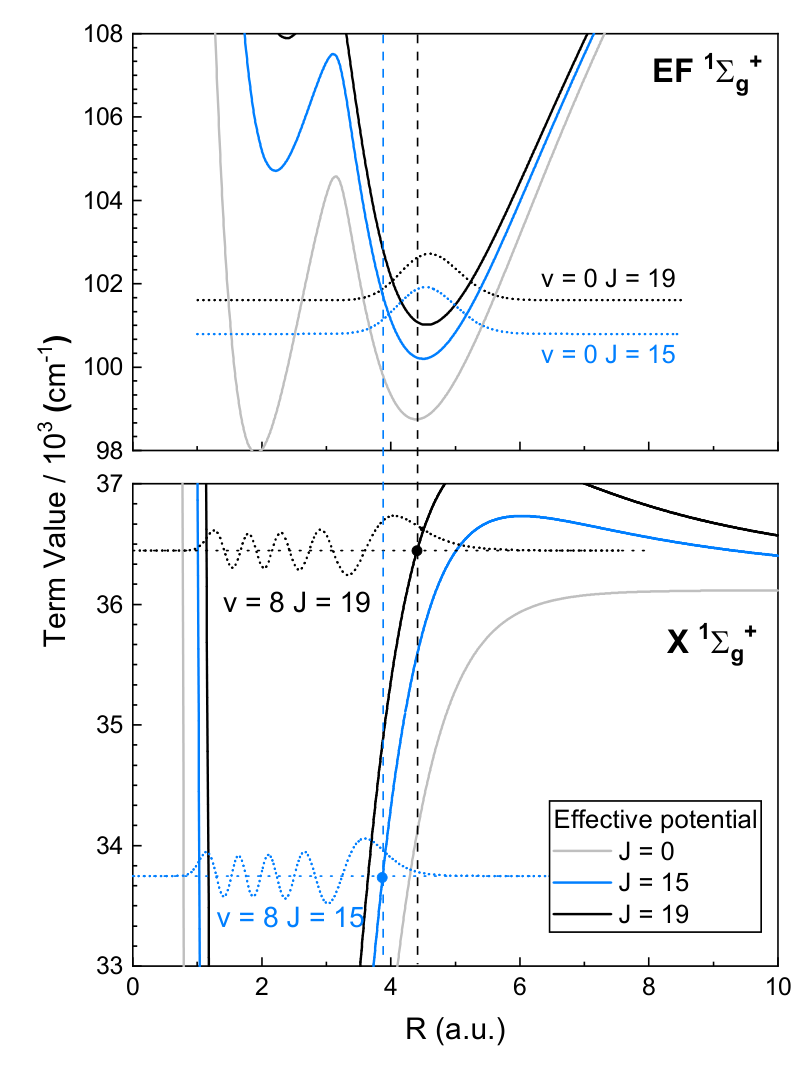
Figure 4 shows how the wave function density at the classical outer turning point of the X state potential provides the overlap with the density on the F well. Vibrational wave functions X() thus provide access to the F outer well, but the subtle overlap make the FC-factors strongly -dependent, since the classical outer turning point extends to larger internuclear distances. As a result, it yields an increasing trend in FC factor with increasing . For moderately high vibrational levels , the FC factors increase with the rotational quantum number for all three isotopologues in the F0-X progression. For lower , the wavefunctions of those moderate high in X states and F0 state are poorly overlapped and give FC factors less than . The Q-branch transitions with a Franck-Condon factor smaller than were discarded in the analysis, as they may be confused with the weaker S-/O-side-branch lines, which are known to be much weaker than the main Q-branch lines in the EF-X two-photon transition in molecular hydrogen Marinero et al. 1983.
Thirdly, combination differences occurring between lines in the spectra were employed. Combination differences exist between S-/Q-/O lines, as well as between vibrational splittings in the X-ground and F-excited states. In the analysis the level energies for the X() ground electronic state as obtained from H2SPECTRE SPE 2022, accurate to within cm-1, are considered to be exact for the purpose of assignment.
As for a fourth ingredient the level energies of F rovibrational states were computed via ab initio methods including non-adiabatic effects. These calculations use improved BO potential energy curves for excited states of molecular hydrogen that have recently become available Siłkowski et al. 2021. The computational methods and results will be presented in section VI. Alongside multi-channel quantum defect (MQDT) calculations Dickenson et al. 2012 were also used to compare with experimental results.
In a few examples, an independent photoionization laser was used for recording autoionization spectra aimed at assigning the rotational quantum numbers of the F-X two-photon transitions Some examples were presented previously Trivikram et al. 2016; Trivikram et al. 2019; Lai et al. 2021a; Lai et al. 2022. However, this additional method is limited to the use of the three-color scheme and too time-consuming to apply it to large numbers of spectral lines.
IV.1 H2

| ac-Stark | ||
|---|---|---|
| Transition | coefficient | |
| F0-X7 Q(21) | 65441.358 (1) | 0.12 |
| F0-X8 Q(19) | 65157.941 (2) | -0.06 |
| F0-X8 S(19) | 65619.860 (1) | 0.00 |
| F0-X8 O(19) | 64734.810 (1) | -0.23 |
| F0-X9 Q(17) | 64837.297 (2) | -0.20 |
| F0-X10 Q(15) | 64493.240 (1) | 0.20 |
| F0-X8 Q(17) | 66044.705 (1) | 0.00 |
| F0-X9 Q(15) | 65571.906 (2) | -0.49 |
| F0-X9 S(15) | 65954.451 (1) | -0.05 |
| F0-X13 Q(5) | 63771.984 (2) | -0.05 |
| F0-X13 Q(3) | 63905.931 (2) | -0.11 |
| F0-X13 Q(1) | 63993.792 (2) | -0.07 |
| F0-X12 Q(4) | 64781.678 (1) | -0.11 |
| F1-X13 Q(0) | 65207.533 (5) | -0.00 |
| F1-X13 Q(1) | 65188.589 (5) | 0.04 |
| F1-X13 Q(2) | 65151.813 (5) | -0.04 |
Several portions of the 2+1 REMPI spectra of the FX system in H2 were presented in previous publications Lai et al. 2021a; Lai et al. 2022. Most of the resonances observed were concentrated between 64 400 - 65 200 cm-1, covering the range of excitations from X12, X13 and X14 levels to F0 and F1 upper levels. Almost all the transitions observed in H ion spectra were also observed via H+ detection.
In Fig. 5 an overview spectrum of the F-X two-photon transitions, as measured via the two-laser scheme, is shown for the region 64 700 - 65 600 cm-1. Here, three lines are indicated that originate in the same X() ground level. The assignment yields direct information on the energy separations between rotational levels in the F0 level. In total 113 lines were observed and assigned in the F()-X() system of H2 through measurement of H+ ion spectra, while 44 lines were observed via H ion detection. In total 118 individual transitions were assigned, in excitation from X() levels to F(). Some 32 and 10 transitions were observed probing F1 and F2 excited vibrations. This coverage of quantum states was limited by the scanning range adopted for the spectroscopy laser.
In the lower panels of Fig. 5 two high-resolution spectra are displayed as recorded in the three-laser scheme exploiting the narrowband PDA system for the spectroscopy step. A list of results obtained via this high-resolution scheme is presented in Table 2. For the lines listed the ac-Stark shift was quantitatively analyzed by performing measurements at differing intensities leading to a determination of ac-Stark slope coefficients, as shown in the insets of Fig. 5. The values for the extracted coefficients are given in the Table as experimental parameters in units of cm-1/mJ. In principle these values could be converted to proper power densities in units of ac-Stark shifts in MHz per MW/cm2, but in view of the large uncertainties in the focal spot size no such conversion will be made and the ac-Stark slope coefficients will only be given in measured units of cm-1/mJ. The regularity of data points in Fig. 5 indicates that the relative values display a convincing degree of consistency.
The ac-Stark slope coefficients appear to exhibit positive and negative values for the different lines. The coefficients reflect the entire level structure of the hydrogen molecule since they involve field-induced couplings over all quantum levels in molecular hydrogen Trivikram et al. 2016. AS such the ac-Stark effect may be considered a high-order moment of the quantum level structure of a molecule. No quantitative theory for these ac-Stark shifts and slope coefficients has been developed. Development of such a theory, tested against experimental parameters would provide information on dynamical polarizabilities of the hydrogen molecule Trivikram et al. 2016. In the literature values have been presented for ac-Stark slope coefficients over several decades, in many cases focusing on the EF-X two-photon transition in H2 Srinivasan et al. 1983; Vrakking et al. 1993; Yiannopoulou et al. 2006; Dickenson et al. 2013; Niu et al. 2014; Trivikram et al. 2016. All resulting values are of order few MHz per MW/cm2, but they appear randomly distributed. The listing of the present large data set on slope coefficients may be useful for benchmarking future theories on the phenomenon.
In previous studies Lai et al. 2021b; Lai et al. 2022, five quasibound resonances on the X-ground state potential have been observed through F0-X transitions: () = (11,13), (10,15), (9,17), (8,19), (7,21). In the present two-color spectra, four of these quasibound resonances, except for (11,13), are again observed in both F0-X and F1-X Q-branch transitions. The absence of the (11,13) quasibound resonance in the two-color spectra may be due to its short 1.6 ns lifetime. In the present study an additional quasibound resonance (6,23) is found through the F0-X6 Q(23) transition at 65678.80 cm-1 as shown in Fig. 6. The calculated excess energy of the (6,23) resonance is 767.79 cm-1, while its lifetime is about 30 s Selg 2012. As discussed in Section II, (6,23) is energetically favourable to be produced upon photolysis of H2S at 281.8 nm. Through the combination difference with the F0-X7 S(21) transition, the ground state interval between (7,21) and (6,23) is 261.15 cm-1, while the calculated value is 261.86 cm-1.


The large set of data on the low-resolution FX two-photon transition frequencies in H2 are listed in Table 11 in the Appendix. For these data the major uncertainty derives from the estimated ac-Stark effect.
IV.2 HD

Spectra of HD were recorded using a premixture of H2S/HDS/D2S gases for the molecular beam. The (2+1) REMPI spectra of the F - X transitions were recorded through H+, D+ and HD+ signal detection. The H+ detected spectra were overwhelmed by the (2+1) REMPI signal from H2 produced from the gas mixture with over 70% of H2S. The signals are produced by H ions from H2 and D+ from HD or D2. Fortunately, these H signals from H2 are sparse in the current scanning range, while the D+ signals from D2 are of low intensity as only 5% of D2S is contained in the precursor mixture. For the analysis of F-X resonances in HD (2+1) REMPI spectra are recorded in separate scans with the ion-mass analyzed set at (probing D+ and H ions) and at (probing HD+). In contrast to the case of H2S large non-resonant background ion signals were detected from the photolysis process. In order to mitigate this and to increase the signal-to-background for the HD spectra, a 1.3 kV/cm dc-field was applied to remove prompt ions.
Fig. 7 shows the HD spectrum in the scan region 63 800 - 64 800 cm-1 for both and ion traces. Many transitions probed at can be assigned to H2 as indicated in the top panel, while a good fraction of the lines is assigned to HD resonances. For HD mostly lines in the F0-X13, F0-X14 and F1-X15 bands are identified. In total 97 lines and 108 lines were observed and assigned in the HD F-X transitions through D+ and HD+ ion spectra respectively. In total 129 individual transitions were labeled with X() levels to F() levels. Similar as in the case of H2, the majority of transitions were assigned as F0-X, amounting to 91 lines observed. Only 10 transitions to F() levels were assigned by the limited spectroscopic laser scanning range and the relatively small Franck-Condon factors, compared to F0-X and F1-X systems. A complete list of transition frequencies in HD is presented in Table 12 in the Appendix.
| Exp. | FT Bailly et al. 2010 | MQDT Dickenson et al. 2012 | NA | ||
| F0 | 0 | ||||
| 1 | |||||
| 2 | |||||
| 3 | |||||
| 4 | |||||
| 5 | |||||
| 6 | |||||
| 7 | |||||
| 9 | |||||
| 11 | |||||
| 13 | |||||
| 15 | |||||
| 17 | |||||
| 19 | |||||
| 21 | |||||
| F1 | 0 | ||||
| 1 | |||||
| 2 | |||||
| 4 |

IV.3 D2
The quality of D2 spectra is inferior to those of the other isotopologues, even though pure D2S was used as precursor in the photolysis. The photolysis of D2S was found to generate large amounts of prompt ions, which were partly removed by applying an opposite polarity dc-field, but still the remaining background lowers the sensitivity of the (2+1) REMPI signals for D2. The scanning range of the spectroscopy laser also covers several absorption bands of the D2S parent molecule, for example the 4 1A2 band at 315 nm and vibronic bands at 302 and 310 nm. Hence the spectroscopy lasers also cause photolysis and the production of various fragment ions. Reducing the pulse energy of the spectroscopy laser was not an option since the 2+1 REMPI signals of D2 would lower the signal-to-noise by too much.
In Fig. 8 spectra of F-X two-photon transitions in the D2 molecule are presented. Three different recordings were performed over the spectral range 64 650 - 65 750 cm-1. With the dissociation laser set at nm many resonances were observed for detection in the D+ signal channel (). This spectrum shows the progressions F0-X() for . For detection in the D channel () only a few marked resonances were observed in this energy range.
In total 93 lines were observed via D+ ion detection and 39 lines via D ion detection. In total 112 individual transitions were assigned to F-X two-photon transitions combining X() ground levels and F() excited levels. The spectra in the D2 measurement appear denser than those for H2 and HD due to its larger moment of inertia. This density limits the assignment of transitions in regions where unresolved bands are observed at poor signal-to-noise ratio. The fact that the lines observed via D detection are erratically distributed may point to a decisive influence of the ionization step, whereby signal is only enhanced for some random lines, where the ionization step matches a transition from the F-state to an autoionizing resonance in the two-color scheme.
In a third spectrum the photolysis laser was moved to nm, while the ion detection was kept at the D channel. Some strong transitions for photolysis at nm are reproduced, while some additional resonances probing lines in the F2-X20 band appear in the spectrum.
From Table 1, the estimated for photolysis of D2S at 281.8 nm is about 97 cm-1, which limits the number of quasibound resonances plausible to form. In the present studies, four quasibound resonances, (13,24), (15,20), (16,18) and (17,15), were observed with resonance energies at about 190, 164, 179 and 31 cm-1, respectively. (15,20) and (17,15) resonances were observed with Q-branch transitions via F0-X15 Q(20) at 64181.15 cm-1, F1-X17 Q(15) at 64624.84 cm-1 and F2-X17 Q(15) at 66507.91 cm-1. However, (13,24) and (16,18) were only observed through the S-/ O-branch transitions. Among the four quasibound resonances, only (17,15) have resonance energy below the of D2S photolysis. The estimated for D2S photolysis has 25 cm-1 uncertainty limited by the experimentally determinated dissociation energy of H2S. From the measurement of D2S photolysis at 259.9 nm with cm-1, F1-X17 Q(15) transition endured in the spectra. However, further proof is needed for the correct assignment of these transitions.
The observed two-photon transition frequencies in the F-X system of D2 are presented in Table 13 in the Appendix.
V F-level energies
The term values for the F outer well rovibrational levels, relative to the X() ground level, can be derived by adding the presently measured two-photon transition frequencies to the calculated term values of ro-vibrational X levels Czachorowski et al. 2018; Pachucki and Komasa 2022. In this procedure a statistical and weighted average is taken over all calibrated two-photon lines probing the same upper level in the F state. A similar approach was followed for the determination of level energies for high rotational states in the E0 - E3 inner well states with up to 19 Dickenson et al. 2012. The accuracy of the X() ground state levels is about cm-1, for some levels at low and even as accurate as cm-1 Hölsch et al. 2019; Puchalski et al. 2019. The accuracy for the highest X() levels was experimentally tested via measurement of combination differences for Lai et al. 2021a.
| State | Exp. | NA. Calc. | MQDT Dickenson et al. 2012 | |
|---|---|---|---|---|
| F0 | 8 | |||
| 10 | ||||
| 12 | ||||
| 14 | ||||
| 16 | ||||
| 18 | ||||
| 20 | ||||
| 23 | ||||
| F1 | 3 | |||
| 5 | ||||
| 611 1 Tentative assignment | ||||
| 7 | ||||
| 8 | ||||
| 9 | ||||
| 10 | ||||
| 12 | ||||
| 13 | ||||
| 14 | ||||
| 15 | ||||
| 16 | ||||
| 17 | ||||
| 19 | ||||
| 21 | ||||
| F2 | 0 | |||
| 1 | ||||
| 2 | ||||
| 3 | ||||
| 5 | ||||
| 6 | ||||
| 7 | ||||
| 9 | ||||
| 11 |
Table 3 lists the thus derived F state term values in H2 as obtained from the accurate three-laser experiments employing the narrow PDA system for the spectroscopy step, while also the ac-Stark effect was addressed quantitatively. Such high-accuracy values are determined for F0 and rotational quantum numbers , restricted to low and for higher- levels to the odd levels in ortho-H2. In addition four term values in F1 were determined for low- values. Table 3 also includes a comparison with experimentally determined energies of F0 and F1 levels form Fourier-transform emission studies Bailly et al. 2010 as well as with a multi-channel quantum-defect (MQDT) calculation for the same levels Dickenson et al. 2013 up to . The differences with the results from the FT-emission data Bailly et al. 2010 are all less than cm-1 and at the level of the combined accuracies, with the exception of the F0() level where the difference is much larger amounting to cm-1.
| State | Exp. | NA. Calc. | |
|---|---|---|---|
| F0 | 0 | ||
| 1 | |||
| 2 | |||
| 3 | |||
| 4 | |||
| 5 | |||
| 6 | |||
| 7 | |||
| 8 | |||
| 9 | |||
| 10 | |||
| 11 | |||
| 12 | |||
| 13 | |||
| 14 | |||
| 15 | |||
| 16 | |||
| 17 | |||
| 18 | |||
| 19 | |||
| 20 | |||
| 21 | |||
| 22 | |||
| 23 | |||
| 24 | |||
| 26 |
In addition to the high-accuracy data extracted from the three-color PDA-based measurements, level energies of some missing rovibrational levels in F0 and F1 states, as well as for F2 were derived from the lower resolution two-color laser measurements. Those results are presented in Table 4. The energies for the F-levels are obtained by averaging over results of measurements of multiple lines in the F-X system. For a subset of 16 levels results for F-level energies as obtained from the high-resolution three-color scheme are compared to results as obtained form the low-resolution two-color laser excitation scheme. The deviations, as plotted in Fig. 9, show that those fall again statistically within the uncertainty of 0.5 cm-1. This proves that the methods of the two-color laser scheme yield F-level energies at an accuracy of 0.5 cm-1. This sets the standard uncertainty for F-levels also in HD and D2 isotopologues.
Similar results for F level energies in HD are presented in Table 5 for the F0 manifold up to , in Table 6 for the F1 manifold up to , while in Table 7 some additional levels pertaining to F2 and F3 are listed.
Results for experimental F level energies in D2 are presented in Table 8 for the F0 manifold observed up to , in Table 9 for the F1 manifold also observed up to , while in Table 10 some levels pertaining to the F2, F3 and F4 manifolds are listed.
| State | Exp. | NA. Calc. | |
|---|---|---|---|
| F1 | 2 | ||
| 3 | |||
| 422 2 Tentative assignment | |||
| 5 | |||
| 6 | |||
| 7 | |||
| 8 | |||
| 9 | |||
| 12 | |||
| 13 | |||
| 14 | |||
| 15 | |||
| 16 | |||
| 17 | |||
| 18 | |||
| 19 | |||
| 22 |
| State | Exp. | NA. Calc. | |
|---|---|---|---|
| F2 | 4 | ||
| 5 | |||
| 7 | |||
| 8 | |||
| 10 | |||
| 14 | |||
| 16 | |||
| F3 | 0 | ||
| 1 |
| State | Exp. | NA. Calc. | Ref. Salumbides et al. 2014. | |
|---|---|---|---|---|
| F0 | 1 | |||
| 2 | ||||
| 4 | ||||
| 5 | ||||
| 6 | ||||
| 7 | ||||
| 8 | ||||
| 9 | ||||
| 10 | ||||
| 11 | ||||
| 12 | ||||
| 13 | ||||
| 14 | ||||
| 15 | ||||
| 16 | ||||
| 17 | ||||
| 18 | ||||
| 19 | ||||
| 20 | ||||
| 21 | ||||
| 22 | ||||
| 23 | ||||
| 2433 3 Tentative assignment | ||||
| 26 | ||||
| 27 | ||||
| 29 |
| State | Exp. | NA. Calc. | Ref. Salumbides et al. 2014. | |
|---|---|---|---|---|
| F1 | 0 | |||
| 2 | ||||
| 3 | ||||
| 4 | ||||
| 5 | ||||
| 6 | ||||
| 7 | ||||
| 8 | ||||
| 10 | ||||
| 11 | ||||
| 12 | ||||
| 13 | ||||
| 14 | ||||
| 15 | ||||
| 16 | ||||
| 17 | ||||
| 19 | ||||
| 20 | ||||
| 21 | ||||
| 22 | ||||
| 23 | ||||
| 24 | ||||
| 26 | ||||
| 29 |
| State | Exp. | NA. Calc. | Ref. Salumbides et al. 2014. | |
|---|---|---|---|---|
| F2 | 0 | |||
| 2 | ||||
| 3 | ||||
| 4 | ||||
| 5 | ||||
| 11 | ||||
| 12 | ||||
| 15 | ||||
| F3 | 8 | |||
| F4 | 7 |
VI Non-adiabatic calculations
To assist the assignment of the 2+1 REMPI spectra for the F-X system, theoretical evaluations for the level energies of F ro-vibrational levels are used, besides those of the highly accurate levels of the X ground state available from non-adiabatic perturbation theory (NAPT) from the H2SPECTRE program suite Czachorowski et al. 2018; SPE 2022. The latter are accurate to cm-1, and can be considered exact for the purpose of comparison with the present experimental data.
The accuracy of ab initio computation of excited state level energies has not reached the same level of accuracy as those for the ground state. However, an extremely accurate calculation was performed in a pre-Born-Oppenheimer framework including relativistic and high-order QED-corrections finding excellent agreement within 0.001 cm-1 for the levels in the E inner well state Ferenc and Mátyus 2019. The Dressler group had previously computed accurate values for the level energies in a non-adiabatic framework Quadrelli et al. 1990; Yu and Dressler 1994. These calculations had reached sub-cm-1 accuracy, and included levels in the F outer well, but the results were limited to low- values.
In an alternative scheme, following the methods of multi-channel quantum-defect theory (MQDT) an accuracy at the level of few cm-1 was achieved for reported levels in the E inner well of H2 Dickenson et al. 2012. Comparison with the present accurate determination of energies for F-levels shows that for F0-levels up to the MQDT-calculations yield values that are all higher by cm-1, and smoothly increasing to an excess of 1.6 cm-1 at . For the low- levels of F1 the MQDT-values are consistently higher by 4.3 cm-1. These comparisons with MQDT results for H2 are displayed in Fig. 10.

For the present assignments and analysis ab initio calculations are performed for ro-vibrational level energies the EF double-well state. We employ the coupled-channel approach described in Ref. Quadrelli et al. 1990 which includes the first five excited states. The term values of the EF() states could be reproduced using the original ab initio data obtained by Wolniewicz and coworkers for the BO potential energy curves, adiabatic corrections and homogeneous electronic coupling functions Yu and Dressler 1994. For the term values presented in this work, the more accurate BO potential energy curves calculated by Silkowski and coworkers Siłkowski et al. 2021 were used, which lowered the energies by about 1 cm-1. Heterogeneous couplings between the EF state and excited were neglected, due to a lack of ab inito data for . This seems justified in view of the 2s character of the EF state and taking into account that a pure precession model predicts only mixing between 3d-3d. For the outer-well F levels with low vibrational excitation, no appreciable 3d character is expected and test calculations including the GK-I heterogeneous coupling result in energy shifts below 0.1 cm-1 even for in H2. Relativistic and QED corrections for E() were found to be of the order of 0.1 cm-1 Ferenc and Mátyus 2019 and were therefore neglected in the current work.
Results of these calculations are included in the various Tables with experimental data on F-levels for H2 (Tables 3 and 4), for HD (Tables 5, 6, and 7) and D2 (Tables 8, 9, and 10).
The calculations of the level energies of the F outer well states can be compared to the level energies assigned from experiment. For this purpose in Fig. 10 a comparison is made between the experimental and theoretical values as obtained for two data sets pertaining to H2. The first panel shows for the high-resolution data in the rotational manifold for F0, a constant offset for the MQDT results, and a gradually increasing offset for the present nonadiabatic calculations as a function of . The smoothness of the curves indicates that there are no outliers that should be interpreted as misassignments.
The second panel of Fig. 10 shows the data for the F1 manifold as obtained from the low-resolution spectra. An outlier is found for the nonadiabatic calculations of the F1() level, which is off by some 2 cm-1, while all other deviations smoothly follow a decreasing trend from low up to a deviation of -3.6 cm-1 at . A similar offset is found in the comparison with MQDT data. In view of this rather strong deviation the assignment of the F1() level in Table 4 is marked as tentative. Indeed, this level was observed in only one transition.
A similar deviation is found for the F1() level in HD, displayed in Fig. 10(c), where the calculated value is higher by 2.8 cm-1, while all other deviations are below 1 cm-1. This assignment for the F0() level in D2, see Fig. 10(d), is also marked as tentative.
The -dependent deviation between experimental and non-adiabatic term values, especially for H2 and HD, indicates missing heterogeneous couplings with excited states, which would lower the theoretical F0 and F1 term values. To improve the coupled-channel calculations, ab inito data for coupling elements is needed. In contrast, MQDT treats homogeneous and heterogeneous nonadiabatic effects naturally on the same footing and the constant offset in Fig. 10 might be reduced drastically by repeating the MQDT calculation with quantum defects extracted from the new ab initio BO potential energy curves.
Recently, the four-body calculations of the inner well E states Ferenc and Mátyus 2019 were extended to the rotational ground state of the outer F well Saly et al. 2023, resulting in a term value of 99365(1) cm-1 for F(0,0). As can be seen from the first entry in Table 3, this deviates by -1.2 cm-1 from the experimental value, compared to a 0.3 cm-1 discrepancy resulting from a comparison with the coupled-channel approach. While four-body calculations allow ultimately to reach higher accuracies, they remain computationally challenging for large and high .
VII Conclusion
In the present study vibrationally and rotationally excited states in the X electronic ground states of H2, HD and D2 fragment species were produced via two-photon ultraviolet photolysis of H2S, HDS and D2S, respectively. These states, with wave function density at large internuclear separation, were subjected to laser spectroscopic investigations of the F - X system in the hydrogen isotopologues. Combined with known accurate theoretical values for the X() levels Czachorowski et al. 2018; Pachucki and Komasa 2022; SPE 2022, level energies of series of rotational states in the F outer well state were determined up to high angular momentum. In H2 results were obtained via a high-resolution three-color laser scheme for at typical uncertainties of cm-1. In addition, from a lower resolution two-color laser scheme additional levels as well as levels were determined at an accuracy of 0.5 cm-1. For HD and D2 energies of many F-levels were determined for the first time.
Full non-adiabatic term values for the F outer well levels were calculated, based on a coupled-channel approach including states. Good agreement, at the level of the experimental accuracy of 0.5 cm-1, is obtained from these calculations.
References
- Dieke (1936) G. H. Dieke, The bands of the hydrogen molecule, Phys. Rev. 50, 797 (1936).
- Dieke (1949) G. H. Dieke, Bands from doubly excited levels of the hydrogen molecule, Phys. Rev. 76, 50 (1949).
- Davidson (1961) E. Davidson, First excited state of the hydrogen molecules, J. Chem. Phys. 35, 1189 (1961).
- Yu and Dressler (1994) S. Yu and K. Dressler, Calculation of rovibronic structures in the lowest nine excited + + states of H2, D2, and T2, J. Chem. Phys. 101, 7692 (1994).
- Shiner et al. (1993) D. Shiner, J. M. Gilligan, B. M. Cook, and W. Lichten, H2, D2, and HD ionization potentials by accurate calibration of several iodine lines, Phys. Rev. A 47, 4042 (1993).
- Zhang et al. (2004) Y. P. Zhang, C. H. Cheng, J. T. Kim, J. Stanojevic, and E. E. Eyler, Dissociation energies of molecular hydrogen and the hydrogen molecular ion, Phys. Rev. Lett. 92, 203003 (2004).
- Hannemann et al. (2006) S. Hannemann, E. J. Salumbides, S. Witte, R. T. Zinkstok, E. J. van Duijn, K. S. E. Eikema, and W. Ubachs, Frequency metrology on the (0,0) transition in H2, HD, and D2, Phys. Rev. A 74, 062514 (2006).
- Salumbides et al. (2011) E. J. Salumbides, G. D. Dickenson, T. I. Ivanov, and W. Ubachs, QED effects in molecules: Test on rotational quantum states of H2, Phys. Rev. Lett. 107, 043005 (2011).
- Dickenson et al. (2012) G. D. Dickenson, E. J. Salumbides, M. Niu, C. Jungen, S. C. Ross, and W. Ubachs, Precision spectroscopy of high rotational states in H2 investigated by Doppler-free two-photon laser spectroscopy in the EF-X system, Phys. Rev. A 86, 032502 (2012).
- Altmann et al. (2018) R. K. Altmann, L. S. Dreissen, E. J. Salumbides, W. Ubachs, and K. S. E. Eikema, Deep-ultraviolet frequency metrology of H2 for tests of molecular quantum theory, Phys. Rev. Lett. 120, 043204 (2018).
- Mulliken (1964) R. S. Mulliken, Rare-gas and hydrogen molecule electronic states, noncrossing rule, and recombination of electrons with rare-gas and hydrogen ions, Phys. Rev. 136, A962 (1964).
- Dressler and Wolniewicz (1984) K. Dressler and L. Wolniewicz, The I state of hydrogen: adiabatic corrections, energy levels, L-uncoupling, and electronic transition moments, Can. J. Phys. 62, 1706 (1984).
- Reinhold et al. (1998) E. Reinhold, A. de Lange, W. Hogervorst, and W. Ubachs, Observation of the I’ outer well state in H2 and D2, J. Chem. Phys. 109, 9772 (1998).
- de Lange et al. (2000) A. de Lange, E. Reinhold, W. Hogervorst, and W. Ubachs, Gerade/ungerade symmetry-breaking in HD at the n = 2 dissociation limit, Can. J. Phys. 78, 567 (2000).
- Sprecher et al. (2013) D. Sprecher, M. Beyer, and F. Merkt, Precision measurement of the ionisation energy of the GK state of H2, Mol. Phys. 111, 2100 (2013).
- Hölsch et al. (2018) N. Hölsch, M. Beyer, and F. Merkt, Nonadiabatic effects on the positions and lifetimes of the low-lying rovibrational levels of the GK and H states of H2, Phys. Chem. Chem. Phys. 20, 26837 (2018).
- Reinhold et al. (1997) E. Reinhold, W. Hogervorst, and W. Ubachs, Observation of a highly excited long-lived valence state in H2, Phys. Rev. Lett. 78, 2543 (1997).
- de Lange et al. (2001) A. de Lange, W. Hogervorst, and W. Ubachs, Double-well states of ungerade symmetry in H2: First observation and comparison with ab initio calculations, Phys. Rev. Lett. 86, 2988 (2001).
- Reinhold et al. (1999) E. Reinhold, W. Hogervorst, W. Ubachs, and L. Wolniewicz, Experimental and theoretical investigation of the state in H2, D2, and HD, and the state in HD, Phys. Rev. A 60, 1258 (1999).
- Detmer et al. (1998) T. Detmer, P. Schmelcher, and L. S. Cederbaum, Ab initio calculations with a nonspherical Gaussian basis set: Excited states of the hydrogen molecule, J. Chem. Phys. 109, 9694 (1998).
- Koelemeij et al. (2003) J. C. J. Koelemeij, A. de Lange, and W. Ubachs, Search for outer-well states above the ionization potential in H2, Chem. Phys. 287, 349 (2003).
- Bailly et al. (2010) D. Bailly, E. Salumbides, M. Vervloet, and W. Ubachs, Accurate level energies in the EF, GK, H, B, C, B’, D, I, J states of H2, Mol. Phys. 108, 827 (2010).
- Salumbides et al. (2014) E. J. Salumbides, D. Bailly, M. Vervloet, and W. Ubachs, B and EF level energies of D2, J. Mol. Spectr. 305, 34 (2014).
- Marinero et al. (1983) E. E. Marinero, R. Vasudev, and R. N. Zare, The E,F double-minimum state of hydrogen: Two-photon excitation of inner and outer wells, J. Chem. Phys. 78, 692 (1983).
- Steadman and Baer (1989) J. Steadman and T. Baer, The production and characterization by resonance enhanced multiphoton ionization of H2 () from photodissociation of H2S, J. Chem. Phys. 91, 6113 (1989).
- Niu et al. (2015) M. L. Niu, E. J. Salumbides, and W. Ubachs, Communication: Test of quantum chemistry in vibrationally hot hydrogen molecules, J. Chem. Phys. 143, 081102 (2015).
- Trivikram et al. (2016) T. M. Trivikram, M. L. Niu, P. Wcisło, W. Ubachs, and E. J. Salumbides, Precision measurements and test of molecular theory in highly excited vibrational states of H2 (), Appl. Phys. B 122, 294 (2016).
- Trivikram et al. (2019) T. M. Trivikram, E. J. Salumbides, C. Jungen, and W. Ubachs, Excitation of H2 at large internuclear separation: outer well states and continuum resonances, Mol. Phys. 117, 2961 (2019).
- Lai et al. (2021a) K.-F. Lai, M. Beyer, E. J. Salumbides, and W. Ubachs, Photolysis production and spectroscopic investigation of the highest vibrational states in H2 (X), J. Phys. Chem. A 125, 1221 (2021a).
- Lai et al. (2021b) K.-F. Lai, , E. J. Salumbides, W. Ubachs, and M. Beyer, Shape resonances in H2 as photolysis reaction intermediates, Phys. Rev. Lett. 127, 183001 (2021b).
- Lai et al. (2022) K.-F. Lai, E. J. Salumbides, M. Beyer, and W. Ubachs, Precision measurement of quasi-bound resonances in H2 and the H + H scattering length, Mol. Phys. 120, e2018063 (2022).
- Quinn et al. (2020) M. S. Quinn, K. Nauta, and S. H. Kable, Disentangling the H2 EF() () - X () () (2+1) REMPI spectrum via 2D velocity-mapped imaging, Mol. Phys. 119, e1836412 (2020).
- Quadrelli et al. (1990) P. Quadrelli, K. Dressler, and L. Wolniewicz, Nonadiabatic coupling between the EF + GK + H, I, and J states of the hydrogen molecule. Calculation of rovibronic structures in H2, HD, and D2, J. Chem. Phys. 92, 7461 (1990).
- Dieke and Lewis (1937) G. H. Dieke and M. N. Lewis, Bands of HD and D2 ending on the state, Phys. Rev. 52, 100 (1937).
- Czachorowski et al. (2018) P. Czachorowski, M. Puchalski, J. Komasa, and K. Pachucki, Nonadiabatic relativistic correction in H2, D2, and HD, Phys. Rev. A 98, 052506 (2018).
- Pachucki and Komasa (2022) K. Pachucki and J. Komasa, Nonrelativistic energy of tritium-containing hydrogen molecule isotopologues, Mol. Phys. 0, e2040627 (2022).
- Ashfold et al. (1990) M. N. R. Ashfold, W. S. Hartree, A. V. Salvato, B. Tutcher, and A. Walker, A reinvestigation of the Rydberg states of H2S and D2S by two-photon resonant multiphoton ionisation spectroscopy, J. Chem. Soc., Faraday Trans. 86, 2027 (1990).
- Zhou et al. (2020) J. Zhou, Y. Zhao, C. S. Hansen, J. Yang, Y. Chang, Y. Yu, G. Cheng, Z. Chen, Z. He, S. Yu, H. Ding, W. Zhang, G. Wu, D. Dai, C. M. Western, M. N. Ashfold, K. Yuan, and X. Yang, Ultraviolet photolysis of H2S and its implications for SH radical production in the interstellar medium, Nat. Comm. 11, 1547 (2020).
- Zhao et al. (2021) Y. Zhao, Z. Luo, Y. Chang, Y. Wu, S. Zhang, Z. Li, H. Ding, G. Wu, J. S. Campbell, C. S. Hansen, S. W. Crane, C. M. Western, M. N. R. Ashfold, K. Yuan, and X. Yang, Rotational and nuclear-spin level dependent photodissociation dynamics of H2S, Nat. Comm. 12, 4459 (2021).
- Tarczay et al. (2001) G. Tarczay, A. G. Császár, O. L. Polyansky, and J. Tennyson, Ab initio rovibrational spectroscopy of hydrogen sulfide, J. Chem. Phys. 115, 1229 (2001).
- Kozin and Jensen (1994) I. Kozin and P. Jensen, Fourfold clusters of rovibrational energy levels for H2S studied with a potential energy surface derived from experiment, J. Mol. Spectr. 163, 483 (1994).
- Miller et al. (1990) S. Miller, J. Tennyson, P. Rosmus, J. Senekowitsch, and I. M. Mills, Calculated rotational and rovibrational spectra of D2S and HDS, J. Mol. Spectr. 143, 61 (1990).
- Ulenikov et al. (1998) O. Ulenikov, G. Onopenko, I. Olekhnovitch, S. Alanko, V.-M. Horneman, M. Koivusaari, and R. Anttila, High-resolution Fourier Transform spectra of HDS in the regions of the bands and , J. Mol. Spectr. 189, 74 (1998).
- Liu et al. (2006) A.-W. Liu, O. Ulenikov, G. Onopenko, O. Gromova, E. Bekhtereva, L. Wan, L.-Y. Hao, S.-M. Hu, and J.-M. Flaud, Global fit of the high-resolution infrared spectrum of D2S, J. Mol. Spectr. 238, 11 (2006).
- Boyarkin et al. (2013) O. V. Boyarkin, M. A. Koshelev, O. Aseev, P. Maksyutenko, T. R. Rizzo, N. F. Zobov, L. Lodi, J. Tennyson, and O. L. Polyansky, Accurate bond dissociation energy of water determined by triple-resonance vibrational spectroscopy and ab initio calculations, Chem. Phys. Lett. 568-569, 14 (2013).
- Niu et al. (2014) M. L. Niu, E. J. Salumbides, G. D. Dickenson, K. S. E. Eikema, and W. Ubachs, Precision spectroscopy of the ) rovibrational splittings in H2, HD and D2, J. Mol. Spectr. 300, 44 (2014).
- Gerstenkorn and Luc (1977) S. Gerstenkorn and P. Luc, Atlas du Spectre d’Absorption de la Molecule d’Iode – cm-1 (Laboratoire Aimé Cotton, CNRS II, 91405 Orsay, France, 1977).
- Wolfsberg et al. (1970) M. Wolfsberg, A. A. Massa, and J. W. Pyper, Effect of vibrational anharmonicity on the isotopic self‐exchange equilibria H2X + D2X = 2 HDX, J. Chem. Phys. 53, 3138 (1970).
- SPE (2022) H2SPECTRE ver 7.4 Fortran source code, University of Warsaw, Poland (2022).
- Siłkowski et al. (2021) M. Siłkowski, M. Zientkiewicz, and K. Pachucki, Accurate Born-Oppenheimer potentials for excited states of the hydrogen molecule, Adv. Quant. Chem. 83, 255 (2021).
- Srinivasan et al. (1983) T. Srinivasan, H. Egger, T. Luk, H. Pummer, and C. Rhodes, The influence of the optical stark shift on the two-photon excitation of the molecular hydrogen EF state, IEEE J. Quant. Electr. 19, 1874 (1983).
- Vrakking et al. (1993) M. Vrakking, A. Bracker, T. Suzuki, and Y. Lee, Ultrasensitive detection of hydrogen molecules by (2+1) resonance-enhanced multiphoton ionization, \rsi 64, 3 (1993).
- Yiannopoulou et al. (2006) A. Yiannopoulou, N. Melikechi, S. Gangopadhyay, J. C. Meiners, C. H. Cheng, and E. E. Eyler, Determinations of EF - X transition frequencies in H2, D2, and HD, Phys. Rev. A 73, 022506 (2006).
- Dickenson et al. (2013) G. D. Dickenson, M. L. Niu, E. J. Salumbides, J. Komasa, K. S. E. Eikema, K. Pachucki, and W. Ubachs, Fundamental vibration of molecular hydrogen, Phys. Rev. Lett. 110, 193601 (2013).
- Selg (2012) M. Selg, Observable quasi-bound states of the H2 molecule, J. Chem. Phys, 136, 114113 (2012).
- Hölsch et al. (2019) N. Hölsch, M. Beyer, E. J. Salumbides, K. S. E. Eikema, W. Ubachs, C. Jungen, and F. Merkt, Benchmarking theory with an improved measurement of the ionization and dissociation energies of H2, Phys. Rev. Lett. 122, 103002 (2019).
- Puchalski et al. (2019) M. Puchalski, J. Komasa, P. Czachorowski, and K. Pachucki, Nonadiabatic QED correction to the dissociation energy of the hydrogen molecule, Phys. Rev. Lett. 122, 103003 (2019).
- Ferenc and Mátyus (2019) D. Ferenc and E. Mátyus, Computation of rovibronic resonances of molecular hydrogen: EF inner-well rotational states, Phys. Rev. A 100, 020501 (2019).
- Saly et al. (2023) E. Saly, D. Ferenc, and E. Mátyus, Pre-Born–Oppenheimer energies, leading-order relativistic and QED corrections for electronically excited states of molecular hydrogen, Mol. Phys. 0, e2163714 (2023).
VIII Appendix
In this Appendix line lists will be provided on the measured frequencies of the F - X two-photon transitions in all three isotopologues, Table 11 for H2, Table 12 for HD, and Table 13 for D2. The listed data are acquired via the low-resolution two-color scheme for which an uncertainty of 0.5 cm-1 is determined.
| Line | Freq. | Line | Freq. | ||||
|---|---|---|---|---|---|---|---|
| 0 | 6 | O(23) | 65178.27 | 0 | 6 | Q(23) | 65678.80 |
| 0 | 7 | Q(19) | 66470.39 | 0 | 7 | Q(20) | 65933.05 |
| 0 | 7 | O(21) | 64978.92 | 0 | 7 | Q(21) | 65441.88 |
| 0 | 7 | S(21) | 65939.95 | 0 | 8 | O(17) | 65662.00 |
| 0 | 8 | Q(17) | 66044.80 | 0 | 8 | Q(18) | 65579.83 |
| 0 | 8 | O(19) | 64734.17 | 0 | 8 | Q(19) | 65157.61 |
| 0 | 8 | S(19) | 65619.98 | 0 | 9 | Q(13) | 66409.96 |
| 0 | 9 | Q(14) | 65983.54 | 0 | 9 | O(15) | 65231.64 |
| 0 | 9 | Q(15) | 65571.25 | 0 | 9 | S(15) | 65954.46 |
| 0 | 9 | Q(16) | 65185.48 | 0 | 9 | S(16) | 65587.59 |
| 0 | 9 | O(17) | 64456.20 | 0 | 9 | Q(17) | 64836.51 |
| 0 | 9 | S(17) | 65260.54 | 0 | 10 | Q(9) | 66400.53 |
| 0 | 10 | Q(10) | 66067.28 | 0 | 10 | O(11) | 65476.88 |
| 0 | 10 | Q(11) | 65728.25 | 0 | 10 | S(11) | 66024.40 |
| 0 | 10 | O(12) | 65116.96 | 0 | 10 | Q(12) | 65392.15 |
| 0 | 10 | O(13) | 64768.88 | 0 | 10 | Q(13) | 65065.84 |
| 0 | 10 | S(13) | 65406.04 | 0 | 10 | O(14) | 64443.43 |
| 0 | 10 | Q(14) | 64761.93 | 0 | 10 | S(14) | 65123.36 |
| 0 | 10 | O(15) | 64152.75 | 0 | 10 | Q(15) | 64493.97 |
| 0 | 10 | S(15) | 64872.86 | 0 | 11 | Q(5) | 65931.85 |
| 0 | 11 | Q(7) | 65510.35 | 0 | 11 | O(8) | 65093.42 |
| 0 | 11 | Q(8) | 65274.82 | 0 | 11 | S(9) | 65281.71 |
| 0 | 11 | Q(10) | 64786.26 | 0 | 11 | S(10) | 65059.98 |
| 0 | 11 | O(11) | 64297.61 | 0 | 11 | Q(11) | 64548.96 |
| 0 | 11 | S(11) | 64845.70 | 0 | 11 | Q(12) | 64331.06 |
| 0 | 12 | Q(3) | 64889.86 | 0 | 12 | S(3) | 64998.96 |
| 0 | 12 | Q(4) | 64781.77 | 0 | 12 | Q(5) | 64654.02 |
| 0 | 12 | S(5) | 64811.24 | 0 | 12 | O(6) | 64376.07 |
| 0 | 12 | Q(6) | 64511.40 | 0 | 12 | O(7) | 64199.67 |
| 0 | 12 | Q(7) | 64357.58 | 0 | 12 | S(7) | 64562.72 |
| 0 | 12 | O(8) | 64024.42 | 0 | 12 | O(9) | 63849.55 |
| 0 | 12 | Q(9) | 64055.69 | 0 | 12 | S(9) | 64305.57 |
| 0 | 12 | O(10) | 63696.70 | 0 | 12 | Q(10) | 63924.40 |
| 0 | 13 | Q(3) | 63905.42 | 0 | 13 | Q(4) | 63841.87 |
| 0 | 13 | O(5) | 63661.97 | 0 | 13 | Q(5) | 63771.65 |
| 0 | 12 | Q(0) | 65060.68 | 0 | 12 | Q(1) | 65032.35 |
| 0 | 12 | O(4) | 64696.16 | 0 | 13 | Q(0) | 64011.54 |
| 0 | 13 | S(0) | 64051.74 | 0 | 13 | Q(1) | 63993.60 |
| 1 | 6 | O(23) | 66308.66 | 1 | 7 | O(21) | 66120.98 |
| 1 | 7 | Q(21) | 66570.35 | 1 | 8 | O(19) | 65887.53 |
| 1 | 8 | Q(19) | 66299.74 | 1 | 9 | Q(16) | 66343.24 |
| 1 | 9 | Q(17) | 65990.07 | 1 | 10 | Q(12) | 66566.23 |
| 1 | 10 | Q(13) | 66236.87 | 1 | 10 | Q(14) | 65928.48 |
| 1 | 10 | Q(15) | 65655.57 | 1 | 11 | Q(8) | 66460.64 |
| 1 | 11 | Q(9) | 66214.56 | 1 | 11 | Q(12) | 65504.24 |
| 1 | 12 | Q(9) | 65238.30 | 1 | 12 | O(10) | 64881.97 |
| 1 | 12 | Q(10) | 65105.98 | 1 | 13 | S(7) | 65027.54 |
| 1 | 12 | Q(7) | 65545.67 | 1 | 13 | Q(0) | 65207.25 |
| 1 | 13 | Q(1) | 65188.76 | 1 | 13 | S(1) | 65247.84 |
| 1 | 13 | Q(2) | 65151.55 | 1 | 13 | O(3) | 65038.08 |
| 1 | 13 | Q(3) | 65099.52 | 1 | 13 | O(5) | 64853.59 |
| 1 | 13 | Q(5) | 64963.13 | 1 | 13 | S(5) | 65116.96 |
| 1 | 13 | Q(6) | 64892.62 | 1 | 13 | O(7) | 64670.11 |
| 1 | 13 | Q(7) | 64825.66 | 1 | 14 | O(4) | 64477.19 |
| 2 | 12 | Q(9) | 66370.16 | 2 | 12 | S(9) | 66610.39 |
| 2 | 13 | S(4) | 66299.74 | 2 | 13 | O(7) | 65807.52 |
| 2 | 13 | Q(7) | 65959.96 | 2 | 14 | Q(1) | 65720.46 |
| 2 | 14 | O(2) | 65675.34 | 2 | 14 | Q(2) | 65711.49 |
| 2 | 14 | S(1) | 65777.95 | 2 | 14 | Q(3) | 65700.67 |
| Line | Freq. | Line | Freq. | ||||
|---|---|---|---|---|---|---|---|
| 0 | 7 | Q(26) | 65910.49 | 0 | 8 | O(24) | 65278.27 |
| 0 | 8 | Q(23) | 66131.28 | 0 | 8 | Q(24) | 65677.54 |
| 0 | 9 | Q(20) | 66237.79 | 0 | 9 | Q(21) | 65808.52 |
| 0 | 9 | Q(22) | 65405.57 | 0 | 9 | Q(23) | 65040.85 |
| 0 | 10 | O(18) | 65512.86 | 0 | 10 | Q(17) | 66208.30 |
| 0 | 10 | O(19) | 65126.52 | 0 | 10 | Q(18) | 65820.40 |
| 0 | 10 | Q(19) | 65449.31 | 0 | 10 | Q(20) | 65101.79 |
| 0 | 10 | Q(21) | 64791.43 | 0 | 10 | S(20) | 65472.05 |
| 0 | 10 | S(21) | 65177.87 | 0 | 11 | O(14) | 65790.64 |
| 0 | 11 | Q(13) | 66369.71 | 0 | 11 | O(15) | 65440.48 |
| 0 | 11 | Q(14) | 66032.76 | 0 | 11 | O(16) | 65097.61 |
| 0 | 11 | O(17) | 64770.99 | 0 | 11 | S(14) | 66307.97 |
| 0 | 11 | Q(16) | 65372.29 | 0 | 11 | O(18) | 64466.84 |
| 0 | 11 | Q(17) | 65063.71 | 0 | 11 | S(17) | 65385.50 |
| 0 | 11 | Q(19) | 64520.56 | 0 | 11 | S(18) | 65113.32 |
| 0 | 12 | O(9) | 66058.38 | 0 | 12 | Q(9) | 66212.27 |
| 0 | 12 | Q(10) | 65960.18 | 0 | 12 | O(12) | 65224.01 |
| 0 | 12 | Q(11) | 65698.30 | 0 | 12 | O(13) | 64942.15 |
| 0 | 12 | Q(12) | 65431.69 | 0 | 12 | O(14) | 64664.34 |
| 0 | 12 | Q(13) | 65165.40 | 0 | 12 | O(15) | 64400.09 |
| 0 | 12 | S(12) | 65673.24 | 0 | 12 | Q(14) | 64905.45 |
| 0 | 12 | O(16) | 64157.36 | 0 | 12 | S(13) | 65423.51 |
| 0 | 12 | Q(15) | 64658.65 | 0 | 12 | Q(16) | 64433.57 |
| 0 | 12 | S(15) | 64951.92 | 0 | 13 | Q(0) | 66102.10 |
| 0 | 13 | Q(2) | 66019.09 | 0 | 13 | Q(3) | 65939.12 |
| 0 | 13 | Q(4) | 65833.49 | 0 | 13 | Q(5) | 65705.22 |
| 0 | 13 | Q(6) | 65557.70 | 0 | 13 | O(8) | 65074.39 |
| 0 | 13 | Q(7) | 65391.40 | 0 | 13 | O(9) | 64867.03 |
| 0 | 13 | Q(8) | 65212.15 | 0 | 13 | O(10) | 64655.98 |
| 0 | 13 | S(7) | 65546.36 | 0 | 13 | Q(9) | 65023.09 |
| 0 | 13 | Q(10) | 64825.92 | 0 | 13 | O(12) | 64229.23 |
| 0 | 13 | Q(11) | 64629.52 | 0 | 13 | O(13) | 64030.79 |
| 0 | 13 | S(10) | 65034.18 | 0 | 13 | Q(12) | 64437.44 |
| 0 | 13 | S(11) | 64855.29 | 0 | 13 | Q(13) | 64255.76 |
| 0 | 13 | S(12) | 64678.28 | 0 | 13 | Q(14) | 64094.35 |
| 0 | 13 | S(13) | 64514.57 | 0 | 14 | O(3) | 64740.57 |
| 0 | 14 | Q(2) | 64848.77 | 0 | 14 | Q(3) | 64785.54 |
| 0 | 14 | Q(4) | 64704.94 | 0 | 14 | Q(5) | 64607.02 |
| 0 | 14 | Q(6) | 64496.31 | 0 | 14 | S(5) | 64725.84 |
| 0 | 14 | Q(7) | 64374.74 | 0 | 14 | Q(8) | 64248.71 |
| 0 | 14 | Q(9) | 64116.85 | 0 | 14 | Q(10) | 63991.87 |
| 0 | 14 | S(9) | 64307.14 | 0 | 14 | Q(11) | 63876.61 |
| 0 | 14 | S(11) | 64101.46 | 0 | 15 | Q(1) | 63986.80 |
| 0 | 15 | Q(2) | 63957.38 | 0 | 15 | Q(3) | 63916.32 |
| 0 | 15 | Q(4) | 63863.43 | 0 | 15 | Q(5) | 63801.30 |
| 0 | 15 | Q(6) | 63736.63 | 1 | 8 | O(24) | 66276.52 |
| 1 | 10 | O(20) | 65776.08 | 1 | 10 | Q(19) | 66456.76 |
| 1 | 11 | Q(16) | 66390.80 | 1 | 11 | Q(17) | 66076.65 |
| 1 | 12 | Q(13) | 66191.40 | 1 | 12 | Q(14) | 65929.67 |
| 1 | 12 | Q(17) | 65255.86 | 1 | 12 | S(17) | 65572.00 |
| 1 | 13 | Q(8) | 66248.12 | 1 | 13 | Q(12) | 65465.48 |
| 1 | 13 | Q(13) | 65282.80 | 1 | 13 | Q(14) | 65121.73 |
| 1 | 13 | S(13) | 65534.97 | 1 | 14 | Q(7) | 65413.09 |
| 1 | 14 | Q(8) | 65284.36 | 1 | 14 | Q(9) | 65152.16 |
| 1 | 14 | O(11) | 64721.76 | 1 | 14 | Q(12) | 64812.33 |
| 1 | 15 | Q(2) | 64999.29 | 1 | 15 | Q(3) | 64958.24 |
| 1 | 15 | O(5) | 64761.69 | 1 | 15 | S(2) | 65059.50 |
| 1 | 15 | Q(5) | 64842.24 | 1 | 15 | Q(6) | 64774.71 |
| 1 | 15 | Q(7) | 64707.07 | 1 | 15 | Q(8) | 64643.85 |
| 1 | 15 | Q(9) | 64591.99 | 1 | 16 | Q(3) | 64413.41 |
| 2 | 12 | Q(16) | 66430.36 | 2 | 13 | Q(14) | 66102.40 |
| 2 | 14 | O(7) | 66294.74 | 2 | 14 | Q(7) | 66410.03 |
| 2 | 15 | Q(8) | 65639.21 | 2 | 15 | S(8) | 65804.57 |
| 2 | 16 | Q(4) | 65396.35 | 3 | 16 | Q(1) | 66400.68 |
| 3 | 17 | Q(0) | 66177.53 |
| Line | Freq. | Line | Freq. | ||||
|---|---|---|---|---|---|---|---|
| 0 | 10 | Q(29) | 65682.19 | 0 | 11 | Q(24) | 66509.52 |
| 0 | 11 | Q(26) | 65787.37 | 0 | 11 | Q(27) | 65449.94 |
| 0 | 12 | Q(20) | 66826.12 | 0 | 12 | Q(21) | 66481.00 |
| 0 | 12 | Q(23) | 65812.66 | 0 | 12 | Q(24) | 65494.50 |
| 0 | 13 | Q(17) | 66647.29 | 0 | 13 | Q(18) | 66345.49 |
| 0 | 13 | Q(19) | 66044.44 | 0 | 13 | Q(20) | 65748.88 |
| 0 | 13 | Q(21) | 65460.65 | 0 | 13 | Q(22) | 65184.22 |
| 0 | 13 | S(24) | 64978.40 | 0 | 14 | Q(17) | 65588.82 |
| 0 | 14 | Q(18) | 65336.29 | 0 | 14 | Q(19) | 65091.05 |
| 0 | 14 | S(17) | 65807.90 | 0 | 14 | S(18) | 65567.20 |
| 0 | 15 | Q(6) | 66766.96 | 0 | 15 | Q(7) | 66627.87 |
| 0 | 15 | Q(8) | 66476.58 | 0 | 15 | Q(9) | 66308.67 |
| 0 | 15 | Q(11) | 65938.80 | 0 | 15 | Q(12) | 65742.01 |
| 0 | 15 | Q(13) | 65537.97 | 0 | 15 | O(16) | 64728.82 |
| 0 | 15 | Q(14) | 65327.24 | 0 | 15 | Q(15) | 65122.32 |
| 0 | 15 | Q(16) | 64914.63 | 0 | 15 | S(14) | 65515.41 |
| 0 | 15 | S(17) | 64933.43 | 0 | 15 | Q(20) | 64181.15 |
| 0 | 16 | Q(5) | 65771.20 | 0 | 16 | O(8) | 65331.49 |
| 0 | 16 | Q(6) | 65668.79 | 0 | 16 | Q(7) | 65551.35 |
| 0 | 16 | Q(8) | 65421.55 | 0 | 16 | Q(9) | 65281.49 |
| 0 | 16 | S(7) | 65655.20 | 0 | 16 | O(12) | 64678.32 |
| 0 | 16 | Q(10) | 65131.89 | 0 | 16 | Q(11) | 64977.58 |
| 0 | 16 | Q(12) | 64816.94 | 0 | 16 | S(10) | 65272.84 |
| 0 | 16 | Q(13) | 64655.44 | 0 | 16 | S(18) | 64166.23 |
| 0 | 16 | Q(4) | 65859.20 | 0 | 17 | Q(5) | 64825.02 |
| 0 | 17 | Q(6) | 64740.84 | 0 | 17 | S(7) | 64749.95 |
| 0 | 17 | O(12) | 63947.24 | 0 | 17 | Q(11) | 64203.54 |
| 0 | 17 | Q(12) | 64088.77 | 0 | 17 | Q(2) | 65000.13 |
| 0 | 17 | Q(4) | 64897.35 | 0 | 18 | S(4) | 64185.23 |
| 0 | 18 | Q(1) | 64219.44 | 0 | 18 | Q(2) | 64195.02 |
| 0 | 18 | S(2) | 64238.44 | 0 | 20 | S(3) | 63267.84 |
| 1 | 10 | Q(29) | 66494.72 | 1 | 11 | Q(26) | 66608.29 |
| 1 | 12 | Q(23) | 66641.46 | 1 | 12 | Q(24) | 66322.34 |
| 1 | 13 | Q(20) | 66584.83 | 1 | 13 | Q(21) | 66294.44 |
| 1 | 13 | Q(22) | 66015.62 | 1 | 14 | Q(16) | 66688.32 |
| 1 | 14 | Q(17) | 66431.15 | 1 | 14 | Q(19) | 65928.48 |
| 1 | 14 | Q(20) | 65691.85 | 1 | 15 | Q(11) | 66789.99 |
| 1 | 15 | Q(12) | 66591.64 | 1 | 15 | Q(13) | 66385.98 |
| 1 | 15 | Q(15) | 65967.18 | 1 | 15 | Q(19) | 65179.15 |
| 1 | 16 | Q(11) | 65828.38 | 1 | 16 | Q(14) | 65339.16 |
| 1 | 16 | Q(17) | 64895.09 | 1 | 16 | Q(4) | 66717.04 |
| 1 | 16 | Q(6) | 66523.54 | 1 | 16 | Q(7) | 66406.87 |
| 1 | 16 | S(6) | 66614.36 | 1 | 17 | O(12) | 64800.23 |
| 1 | 17 | Q(10) | 65171.10 | 1 | 17 | Q(11) | 65052.64 |
| 1 | 17 | Q(12) | 64937.89 | 1 | 17 | Q(15) | 64624.84 |
| 1 | 18 | S(8) | 64831.26 | 1 | 18 | S(9) | 64769.49 |
| 1 | 18 | Q(2) | 65052.23 | 1 | 18 | Q(3) | 65017.30 |
| 1 | 18 | Q(4) | 64973.60 | 1 | 18 | Q(5) | 64920.35 |
| 1 | 18 | Q(6) | 64858.44 | 1 | 18 | Q(7) | 64790.97 |
| 1 | 18 | Q(8) | 64717.59 | 1 | 19 | O(8) | 64170.87 |
| 1 | 20 | Q(0) | 64082.43 | 2 | 17 | Q(5) | 66507.91 |
| 2 | 17 | Q(11) | 65879.61 | 2 | 17 | Q(12) | 65760.99 |
| 2 | 17 | Q(15) | 65446.28 | 2 | 18 | Q(2) | 65883.04 |
| 2 | 18 | Q(3) | 65845.22 | 2 | 18 | Q(4) | 65802.74 |
| 2 | 19 | Q(4) | 65229.39 | 2 | 20 | Q(0) | 64910.20 |
| 3 | 19 | Q(8) | 65889.37 | 4 | 19 | S(5) | 66846.32 |