The fermion-boson map for large $d$ and its connection to lattice transformations

Three-dimensional bosonization physics [1] via statistical transmutation [2, 3] is a very interesting and recurrent subject in field theory and condensed matter physics, and it has been connected (see e.g. [4, 5, 6, 7, 8]) to particle-vortex duality e.g. [9]. The extension of fermion-boson duality to finite temperature thermal field theory has also been considered (see for example [10, 11] and references therein), in the context of various models that describe matter coupled to non-abelian Chern-Simons fields but also the more recent works about exploring the symmetry-breaking of conformal theories in the large-charge limit like [20]. Those works present a remarkable progress in our understanding of three-dimensional physics, and its possible holographic higher-spin duals.

Since fermion-boson duality is a fundamental property of three-dimensional quantum physics one may think that it is not necessary to invoke non-abelian gauge fields to make it manifest. Having this idea in mind we revisited in [12, 13] the finite temperature phase structure of two 3$d$ and odd $d$ systems in general; the fermionic $U(N)$ Gross-Neveu model and the bosonic CP^N-1 model. We have studied those systems in the canonical formalism by introducing an imaginary chemical potential as a $U(1)$ charge. In such a setup the large-$N$ canonical partition functions are intimately related to the partition functions of the same systems coupled to an abelian Chern-Simons gauge field expanded around a monopole background in a suitable mean field approximation [15]. Also, the imaginary $U(1)$ charge density is related to the Chern-Simons level. The generalization of $3d$ theories to arbitrary $odd$ dimensions at finite temperature and imaginary chemical potential is hard due to the non renormalizability of the corresponding models, nevertheless a precise map of their gap equations, free energies and partition functions was demonstrated for a certain region of their phase space [12, 13]. The non renormalizability of our models can be tamed by introducing a lattice field-like theory based on Bloch-Wigner-Ramakrishnan functions $D_{d}(z)$ [16, 19]. Our calculations have unveiled the relevance of these functions to the physics of the fermion-boson map and we have argued that there is a non-trivial large $d$ limit of the fermion-boson map which at the level of partition functions is expressed by a general formula with a special characteristic which is the basis for this work.

I begin with a generalization of the Bragg Law of diffraction in Section 2 and I continue with a brief introduction to generic notes about statistical transmutations and the phase transitions of a fermionic theory at imaginary chemical potential in section 3. I continue with a brief review of the three-dimensional and general $odd$ dimensions results of [12, 13] in Section 4. In particular, I discuss that when I introduce an imaginary chemical potential the phase structures of the Gross-Neveu and CP^N-1 models are characterised by the presence of thermal windows inside which the systems do not have definite fermionic or bosonic properties. The edges of the thermal windows are inflection points of the free energies, while in the middle points of the above windows the systems appear to have completely switched statistics i.e. the fermionic becomes bosonic and vice versa. Encouraged by the odd $d$ analysis I found a remarkable result at the $d\rightarrow\infty$ that points towards particles that travel inside a lattice [14]. Nevertheless, the edges of the higher-dimensional thermal windows are also inflection points of the free energy and they correspond to zeros and extrema of the $D_{d}(z)$ functions with $odd$ and even $d$ respectively. This pattern continues for all odd $d$. In previous work we were able to give an analytic formula for the approximate positions of those saddle points in the form of a sequence of rational multiples of $\pi$ that lie between $\pi/3$ and $\pi/2$. As $d\rightarrow\infty$ those points accumulate near $\pi/2$ and the relevant $D_{d}(e^{i\theta})$ function becomes simply $\sin(\theta)$. This observation allowed us to ask whether the fermion-boson map has a well defined large $d$ limit, and indeed we argued that for models with supersymmetric matter content the partition function duality formula (51) goes to the simpler one (52).

In Section 5 I discuss the main idea of this work where I make the connection of the $U(1)$ charge to a lattice transfer momentum and insert the idea of the hexagons and quadrilaterals conjectures in order to find a correspondence between the generalized thermal windows and the lattice points of specific lattices. In section 6 I examine in detail the setup of the higher dimensional thermal windows for fermions and bosons and the correspondence of the lattices constructions of the conjectures that are the basic idea of the paper. In Section 7 I present a new idea of considering the fermion and boson partition functions as Bloch waves and at Section 8 I discuss the relevance of the strong coupling regime with hexagons and quadrilaterals conjectures which is a new method of lattice regularization. I summarise and offer a few ideas for future work in Section 9. An Appendix contain some technical details and useful formulae for Bloch-Wigner function.

In physics, Bragg’s Law of diffraction is a special case of Laue diffraction, which gives the angles of the scattering from a crystal lattice. When a beam of particles with a wavelength comparable to atomic space between the atoms of a crystal is scattered by a lattice plane, the incidental and the reflected waves remain in phase since the difference between their path lengths is equal to an integer multiple of their wavelength. This path difference between the two waves undergoing interpolation is given by $2d\sin\theta$, where $\theta$ is the scattering angle and $d$ is the interplanar distance.

So, this integer multiple of the wavelength is giving the Bragg’s Law as

My analysis will focus on the transfer momentum of the scattering on a hexagonal and regular triangle surface of a crystal and its transformations to a square lattice [38, 39]. If we accept that the atoms of the crystal remain fixed, then the change in the incident particle’s momentum will be equal to $p_{i}-p_{f}$ where $p_{i},p_{f}$ the initial and final momentum respectively. A wave has a momentum $p=\hbar k$ and is a vectorial quantity. The wave number $k$ is the absolute of the wave vector $k=p/\hbar$ and is related to the wavelength $k=2\pi/\lambda$. Frequently, momentum transfer is given in wavenumber units in reciprocal length $Q=k_{f}-k_{i}$. The momentum transfer plays an important role in the evaluation of neutron, X-ray and electron diffraction for the investigation of condensed matter. Bragg diffraction refers to the atomic crystal lattice, conserves the wave energy and thus is called elastic scattering, where the wave numbers of the final and incident particles, $k_{f}$ and $k_{i}$, respectively, are equal and since only the direction changes, we calculate a reciprocal lattice vector $G=Q=k_{f}-k_{i}$ with the relation to the lattice spacing $G=2\pi/d$. When momentum is conserved, the transfer of momentum corresponds to crystal momentum.

The presentation in $Q$-space is generic and does not depend on the type of the beam and wavelength used but only on the sample system, which allows to compare the results we obtained from different scattering methods. Then the overall transfer momentum from N particles will be (Figure 1)

It is obvious that the maximum transfer momentum happens when the angle between the direction of the velocity of the particles and the direction that connects two neighbor atoms horizontally is $\pi/2$. We may write $sin\theta$ like:

the lattice space as $d$ and the wavelength as $\lambda$. The above sum goes to zero at the limit where $n\rightarrow\infty$.

Suppose now that we define a new function $\Omega$ where

for arbitrary even $m=2,4,...,\infty$. This $\Omega$ function is Clausen function $Cl_{m}(\theta)$. So the Bragg Law of diffraction of a perturbed lattice with lattice space $d^{{}^{\prime}}$ may have a generalised version in arbitrary dimensions:

where $dsin\theta=d^{{}^{\prime}}\Omega(\theta)$. The sum in the parenthesis is the Clausen function so:

The transferred momentum is

where $G$ is the reciprocal lattice vector with $G=2\pi/d^{{}^{\prime}}$. For $n=1$, $\lambda=1$ and $N$ beam particles we have:

Since I have argued before that the charge density $Q$ may represent the lattice momentum difference between two wave-functions or the lattice operator that "drives" the incident beam condition to the reflected one, my attention will focus on an equation from our previous work [13].

I briefly review the relationship of the imaginary chemical potential to statistical transmutation [33, 34] considering for example the fermionic theory. It is easy to see that the presence of the imaginary chemical potential can be cancelled by an abelian gauge transformation for the fermions like:

However, at finite temperature the fermions are anti-periodic on the thermal circle

We then see that the gauge transformed fields would satisfy

Hence, the anti-periodic boundary conditions are preserved only if $\theta=2\pi n$, $n\in\mathbb{Z}$. Other values of $\theta$ would "twist" the boundary conditions and change the statistics of the underlying system. A similar argument goes through for bosonic systems where the complex scalars satisfy periodic boundary conditions on the thermal circle. The twisting of the thermal boundary conditions is the main underlying mechanics behind the possible statistical transmutation in systems whose grand canonical potential is extremized at non trivial values of the imaginary chemical potential.

The calculation of the canonical partition function in systems with global $U(1)$ charges appears to be agnostic to their underlying microscopic structure e.g. whether the elementary degrees of freedom carrying charge are bosonic or fermionic. Indeed, it looks like that the only useful piece of information one has is the kind of periodicity of the partition function, something that could just give a hint regarding the presence of a confinement/deconfinement transition.

The situation resembles studies of quantum mechanical systems in a periodic potential like a periodic crystal. If we think of $\theta$ as a periodic coordinate, then is equivalent to the calculation of the overlap between two Bloch wavefunctions that differ by lattice momentum $Q$ [24]. Such systems usually generate a band structure which can be studied by restricting the lattice momentum to the first Brillouin zone. Although one generally cannot go very far without using a particular microscopic model at hand, there are certain topological properties of a single band such the eigenvalues of the Zak phase [25], which hold physically relevant information of the system i.e. polarization. I will pursue further this line of ideas later and if there is a lesson to be learned is that there may be some universal features of generic quantum systems in periodic potentials which are independent of their fermionic or bosonic microstructure. Hence, a fermion-boson map appears to be generic. This will be reviewed below by considering two explicit odd dimensional models: the $U(N)$ fermionic Gross-Neveu and the bosonic CP^N-1 model and the transformations of two lattices, the hexagonal and the triangular.

It is well known that in the absence of a chemical potential $U(N)$ fermionic Gross-Neveu and CP^N-1 models exhibit very different patterns of symmetry breaking at finite temperature $T$. The Gross-Neveu model has a parity broken phase at low temperatures, which disappears for a critical temperature. On the other hand, while the CP^N-1 model exhibits the usual continuous symmetry breaking pattern at zero temperature, the broken phase ceases to exist for $T>0$ in accordance to the Mermin-Wagner-Colleman theorem that forbids continuous symmetry breaking at finite $T$ for two-dimensional systems. What instead happens is that when the coupling is tuned to its critical value at $T=0$, then a finite temperature scaling regime with a non-zero thermal mass for the scalars emerges. I nevertheless have shown in [12] that the situation changes in the presence of the imaginary chemical potential, and the corresponding phase structures of the two models can be mapped into each other. I have further observed in [12] the relevance of the celebrated Bloch-Wigner function [16] in our calculations of the gap equations and free energies which for $d$-odd can be expressed as finite sums of Nielsen’s generalized polylogarithms [12, 31, 32], while for $d$-even the corresponding expressions are much more complicated. Moreover, I have already noted the relevance of the 1$d$ theories to the physics of the the 3$d$ models. For these reasons, I will concentrate on studying the generalizations of our 3$d$ models to odd $d>3$. This mathematical curiosity, together with the aim to shed more light into the physics of bosonisation, prompted me to study the fermion-boson map in higher dimensions in[13] and to extend my thinking to the correlation of the phase transformations of our continuum models with the transformations of specific lattices where they show remarkable similarities and correspondences, with the help of the zeros and maximizations of Bloch-Wigner functions introduced by Zagier. The two models in arbitrary odd dimensions are:

As we have seen before in [13]

where $Z^{(3)}_{f}$ ($Z^{(3)}_{b}$) denote the $3d$ fermionic (bosonic) canonical partition function. I have kept the ${\rm Tr}{\mathbb{I}}_{2}$ explicitly in order to compare with the corresponding formula for general $d$ that will be given later. The total partition function plays the role of the generating function of all correlation functions. The above equation may be interpreted as giving the difference between the momentum of an incoming and outgoing beam when it scatters from a lattice point and the only change that happens is in the direction. Since the exponential is imaginary (I take the imaginary part of the charge) the above gives us a scattering-like procedure of a Bloch-wave kind beam on a lattice point. When $\beta\alpha_{*}=0,\pi$, then $Q_{3}=q_{3}=0$ and the above is the well-known statement of fermion/boson duality i.e. the twisted fermionic (namely, imposing period boundary conditions) and the bosonic partition functions are inverse one of the other. However, for $Q_{3},q_{3}\neq 0$ the corresponding partition functions are weighted duals due to the presence of the real exponential in the r.h.s. of the above equation. We can give an interpretation of that latter weight factor recalling that the gap equations of charge for the Gross-Neveu and the $CP^{N-1}$ models tie $Q_{3}$ and $q_{3}$ to the Bloch-Wigner function $D_{2}(z)$, and hence to the volume of hyperbolic manifolds. Then the above could be understood as giving the leading "classical" term in a perturbative expansion of a complex Chern-Simons action in inverse powers of the level. Support for such an interpretation also comes from the fact that the extremal values that we have found for the fermionic and bosonic imaginary charges, coincide with the results reported in the study of the partition function of the $SL(2,\mathbb{C})$ CS theory [26, 27, 17, 18] where a complex hyperbolic volume is a combination of a gravity hyperbolic volume together with the Chern-Simons invariant

where from my point of view we are dealing with the hypervolume-gravity part when we calculate odd index $D(z)$ functions and a Chern-Simons part when we calculate the even index $D(z)$ functions like the charge $Q$, which is similar with the Chern-Simons part of past works in which theoretically fermionic or bosonic matter was coupled to a Chern-Simons gauge field. On the other hand, it is also tempting to interpret the above as a "generalized Wilson line" i.e. an overlap between Bloch states at different quasimomenta. The Wilson line operator describes the transport of a Bloch state from quasimomentum $Q$ to $q$. In such a case, the partition functions would correspond to complex conjugate Bloch wave functionals, and the charges $Q_{3}$ or $q_{3}$ would play the role of quasimomenta. This hypothesis will be enhanced by the analysis of the next section. Finally, in previous work we have also suggested a geometric interpretation for this result. Namely, that the bosonic and fermionic free energies at imaginary chemical potential correspond to partial volumes of an ideal tetrahedron. Their sum gives the entire volume.

Based on the hypothesis I had previously, I can, in line with the generalization of the thermodynamic study of Gross-Neveu and CP^N-1 theories, give a more general hypothesis on the total particles (that scattered from a lattice) value of the transfer momentum. I have seen that the exponent of the total partition function of a supersymmetric model from charged fermions and bosons gives us the total transfer momentum that occurs when these particles are scattered by a crystal with a hexagonal unit lattice. This is based on the fact that the inner angles of a regular hexagon are exactly $2\pi/3$ so the maximization of the transfer momentum coincides with the maximization of the Clausen function which is equal to the imaginary part of $Li_{2}(-z)$ on the unit circle. If we look for the corresponding maximization for the charge/momentum at $5,7,9$ .. dimensions we observe that this occurs for specific angles of incidence $7\pi/13$,$26\pi/51$,$103\pi/205$ and so on. These values come from an analytic formula for the approximate positions of the zeros of all $D_{2n-1}(z)$, $n=1,2,..$ functions on the unit circle. We obtain:

where

for $n=1,2,3,..$. There is an interesting approximation of these zeros in [21].

The particles see specific surfaces on Euclidean space with the first Brillouin zones of them including irregular hexagons. At a large $d$ limit the conjecture ends up to the square lattice construction. Somehow as dimension increases the 6th and 5th sides disappear. The conjecture turns to be as follows:

Let’s see a way to construct these hexagons by using the golden ratio generalized polynomial.

• •

  Figure 2

$AF=AW=\alpha,WL=WO=\sqrt{2}\alpha$, $\frac{AW}{sin\omega}=\frac{AL}{sin\theta}=\frac{WL}{sin2\pi/3}\rightarrow\frac{\alpha}{sin\omega}=\frac{AL}{sin\theta}=\frac{WL}{sin2\pi/3}=\frac{2\sqrt{6}\alpha}{3}$, so $sin\omega=\frac{\sqrt{6}}{4}$, where $\omega$ is the angle between AL and WL and $\theta$ is the angle between AW and WL. Also, $sin^{2}\omega+cos^{2}\omega=1\rightarrow cos\omega=\frac{\sqrt{1}0}{4}$. But $\theta+\omega=\frac{\pi}{3}\rightarrow$

$sin\theta=sin(\frac{\pi}{3}-\omega)\rightarrow sin\theta=sin\frac{\pi}{3}\cdot cos\omega-cos\frac{\pi}{3}\cdot sin\omega=\frac{\sqrt{6}}{8}(\sqrt{5}-1).$

So, $AL=sin\theta\cdot\frac{2\sqrt{6}\alpha}{3}=\frac{(\sqrt{5}-1)\alpha}{2}=\frac{\alpha}{\phi}$. At the end we find that

with the corresponding hexagonal lattice (Figure 2).

• •

  Figure 3

$AF=AW=\alpha,WL=WO=\sqrt{2}\alpha$

$\frac{AW}{sin\omega}=\frac{AL}{sin\theta}=\frac{WL}{sin7\pi/13}\rightarrow\frac{\alpha}{sin\omega}=\frac{AL}{sin\theta}=\frac{WL}{sin7\pi/13}=1.4246\alpha$, so $sin\omega=0.70195$. Also, $sin^{2}\omega+cos^{2}\omega=1\rightarrow cos\omega=0.712225$. But $\theta+\omega=\frac{6\pi}{13}\rightarrow$

$sin\theta=sin(\frac{6\pi}{13}-\omega)\rightarrow sin\theta=sin\frac{6\pi}{13}\cdot cos\omega-cos\frac{6\pi}{13}\cdot sin\omega=0.622415.$

So, $AL=sin\theta\cdot 1.4246\alpha=0.8866925\alpha$. At the end we find that

where we have an approximation of $93.41\%$.

• •

  Figure 4

$AF=AW=\alpha,WL=WO=\sqrt{2}\alpha$

$\frac{AW}{sin\omega}=\frac{AL}{sin\theta}=\frac{WL}{sin26\pi/51}\rightarrow\frac{\alpha}{sin\omega}=\frac{AL}{sin\theta}=\frac{WL}{sin26\pi/51}=1.414885\alpha$, so $sin\omega=0.7067712$. Also, $sin^{2}\omega+cos^{2}\omega=1\rightarrow cos\omega=0.7074418$. But $\theta+\omega=\frac{25\pi}{51}\rightarrow$

$sin\theta=sin(\frac{25\pi}{51}-\omega)\rightarrow sin\theta=sin\frac{25\pi}{51}\cdot cos\omega-cos\frac{25\pi}{51}\cdot sin\omega=0.6853407.$

So, $AL=sin\theta\cdot 1.414885\alpha=0.9696782\alpha$. At the end we find that

where now we have a better approximation of $99.45\%$.

The next candidate Brillouin zone of the hexagons’ conjecture gives a ratio

where the approximation is $99.93\%$. Finally we have the first Brillouin zone of the square lattice with the ratio

It is very interesting that the value of the golden ratio and Riemann $\zeta$ functions are connected to each other from the generalized golden ratio formula like:

with $n=1,2,3\dots$, creating a "family" of first Brillouin zones whose construction is based on $\zeta$ functions and the golden ration $\phi$.

For example if $n=1$ then the golden ratio equation becomes: $x-2=0\rightarrow x=2$ and $x-1=1$ (square lattice). If $n=2$ then the generalized golden ratio equation becomes: $x^{2}-x-1=0\rightarrow x=\frac{1+\sqrt{5}}{2}\rightarrow x-1=\frac{1}{\phi}$ (honeycomb lattice). This motive continues like for $n=3$ and $x-1=\frac{1}{\zeta(3)}$, for $n=5$ we have $x-1=\frac{1}{\zeta(5)}$, etc. These are the values of the ratios

$n=3,5,7,\dots$ for all the pertubed lattices coming from the regular hexagonal lattice.

There is also a similar construction of the first Brillouin zones of the triangular dual lattices that correspond to the $CP^{N-1}$ bosonic model at imaginary chemical potential. The first Brillouin zone of the triangular lattice corresponding to Figure 2 is the one of Figure 5. We see now that there is another thermal window of the fermionization of the model.

• •

  Figure 5

$AF=AW=\alpha,WL=WO=\sqrt{2}\alpha$, $\frac{AW}{sin\omega}=\frac{AL}{sin\theta}=\frac{WL}{sin\pi/3}\rightarrow\frac{\alpha}{sin\omega}=\frac{AL}{sin\theta}=\frac{WL}{sin\pi/3}=\frac{2\sqrt{6}\alpha}{3}$, so $sin\omega=\frac{\sqrt{6}}{4}$, where $\omega$ is the angle between AL and WL and $\theta$ is the angle between AW and WL. Also, $sin^{2}\omega+cos^{2}\omega=1\rightarrow cos\omega=\frac{\sqrt{1}0}{4}$. But $\theta+\omega=\frac{2\pi}{3}\rightarrow$

$sin\theta=sin(\frac{2\pi}{3}-\omega)\rightarrow sin\theta=sin\frac{2\pi}{3}\cdot cos\omega-cos\frac{2\pi}{3}\cdot sin\omega=\frac{\sqrt{6}}{8}(\sqrt{5}+1).$

So, $AL=sin\theta\cdot\frac{2\sqrt{6}\alpha}{3}=\frac{(\sqrt{5}+1)\alpha}{2}=\alpha\phi$. At the end we find that

with the corresponding triangular lattice (Figure 5).

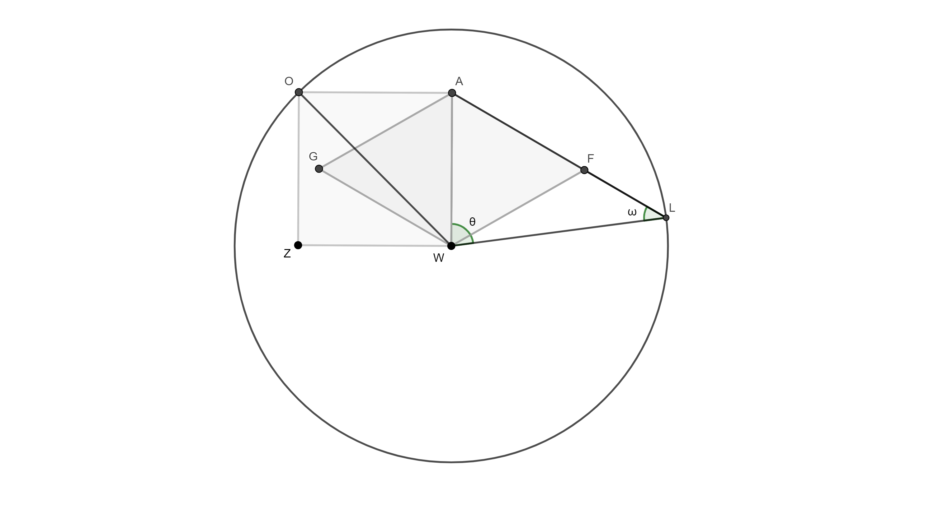
The next lattice (Figure 6) is:

$AF=AW=\alpha,WL=WO=\sqrt{2}\alpha$, $\frac{AW}{sin\omega}=\frac{AL}{sin\theta}=\frac{WL}{sin6\pi/13}\rightarrow\frac{\alpha}{sin\omega}=\frac{AL}{sin\theta}=\frac{WL}{sin6\pi/13}=1.4246\alpha$, so $sin\omega=0.70195$, where $\omega$ is the angle between AL and WL and $\theta$ is the angle between AW and WL. Also, $sin^{2}\omega+cos^{2}\omega=1\rightarrow cos\omega=0.712225$. But $\theta+\omega=\frac{7\pi}{13}\rightarrow$

$sin\theta=sin(\frac{7\pi}{13}-\omega)\rightarrow sin\theta=sin\frac{7\pi}{13}\cdot cos\omega-cos\frac{7\pi}{13}\cdot sin\omega=0.791651474.$

So, $AL=sin\theta\cdot 1.4246\alpha=1.12778669\alpha$. At the end we find that

which is exactly the inverse of the result of the corresponding transformed hexagonal lattice (Figure 3).

This motive continuous but now we are inetrested in $\frac{1}{x-1}$ solutions of equation $x^{n}-x^{n-1}-x^{n-2}-\dots-1=0$. These are $\phi,\zeta(3),\zeta(5),\dots,\zeta(\infty)$.

Since I show that the $Gross-Neveu$ and $CP^{N-1}$ models at imaginary chemical potentials are duals for a specific shift of the chemical potential we may say that fermions and bosons "see" the dual lattices as they move on the surfaces of them.

Tables 1 and 2 seems to be clearly in agreement with equation (8), where at infinite dimensions the total transfer momentum of the fundamental particles is equal to the overall transfer momentum of the modified Bragg Law, apart from a factor arising from the compact dimension on the thermal circle that disappears at infinite dimensions. Although I go physically to higher dimensions, it can be reverted to a study of 2 + 1 dimensions by scattering into hypothetical crystals, which (with very good approximation) give us the changes of the momentum of the scattered particles. We also have to mention that we will have the same results if we use the angles $6\pi/13$, $25\pi/51$, $102\pi/205$.. with the corresponding quadrilaterals of our conjecture where the first Brillouin zone of the family is the one of the triangular lattice (dual lattice) and the construction is made of tetrahedra instead of hexagons. Like before the "infinite dimensional theory" construction turns to a square/rectangle tiling of the original Bragg Law.

It is also interesting that there are two kind of functions that become from the ratio $\frac{AL}{AF}$ and take values

where $K=1,\phi,\zeta(3),\zeta(5)\dots$. The product of these functions

is a normalization value that equals to $1$ for the $3d$ case and also for the other cases. The ratios are almost $\zeta(n)$ or $\frac{1}{\zeta(n)}$ and this may come from the fact that theories in higher dimensions are non-renormalizable and the lattices that arise from the conjectures do not have normal polygons. I conjugate that this product gives the duality picture of the hexagonal and triangular lattices. It is like the duality image of a fermionic and bosonic theory where their partition functions are inverse one of the other.

One may see the transformation of a triangular lattice to a hexagonal one and compare with the phase transitions of the Gross-Neveu model at imaginary chemical potential. The picture is like the one that follows:

”Studying the correspondence of thermal windows with the transformation of a hexagonal to triangular lattice we have fermions at a high temperature and freeze them until we reach a critical temperature where we go to boson condensates. The thermal window closes at a lower temperature and we have fermions again. Respectively in some hexagonal materials we have phase transitions with a broken symmetry where triangular materials are arising (like the FCC to BCC transformations).”

Let’s see in detail Figure 2. We have a circle with radius $\sqrt{2}a$ that intersects segment $AF$ at $L$ point. Interestingly there is an equivalent picture of the thermal windows in the Gross-Neveu model at finite T and imaginary chemical potential. In the Gross-Neveu model and its change in the statistics we have temperature (the chemical potential) that "creates" the thermal windows, where inside them we have a chiral symmetry breaking in order to make some fermion condensates. In our conjecture the thermal windows have the equivalent picture of the region inside the hexagon. As we will see later the borders of the thermal windows coincides with the positions of the lattice points of the hexagon. At these points, $D_{2}(-z*)$ has its maximum value. The lattice point D is the equivalent point of the full bosonization in the Gross-Neveu model. The points L and F are coming closer and at $d\rightarrow\infty$ they coincide. One may say it seems that at infinite dimensions symmetry is always unbroken and we return to a fermionic theory.

The generalised thermal windows are:

References

- [1] E. H. Fradkin and F. A. Schaposnik, The Fermion - boson mapping in three-dimensional quantum field theory, Phys. Lett. B338 (1994) 253–258, [http://arxiv.org/abs/hep-th/9407182].
- [2] F. Wilczek, Magnetic Flux, Angular Momentum, and Statistics, Phys. Rev. Lett. 48 (1982) 1144–1146.
- [3] A. M. Polyakov, Fermi-Bose Transmutations Induced by Gauge Fields, Mod. Phys. Lett. A3 (1988) 325.
- [4] A. Karch and D. Tong, Particle-Vortex Duality from 3d Bosonization, Phys. Rev. X6 (2016), no. 3 031043, [http://arxiv.org/abs/1606.01893].
- [5] J. Murugan and H. Nastase, Particle-vortex duality in topological insulators and superconductors, JHEP 05 (2017) 159, [http://arxiv.org/abs/1606.01912].
- [6] N. Seiberg, T. Senthil, C. Wang, and E. Witten, A Duality Web in 2+1 Dimensions and Condensed Matter Physics, Annals Phys. 374 (2016) 395–433, [http://arxiv.org/abs/1606.01989].
- [7] S. Kachru, M. Mulligan, G. Torroba, and H. Wang, Bosonization and Mirror Symmetry, Phys. Rev. D94 (2016), no. 8 085009, [http://arxiv.org/abs/1608.05077].
- [8] O. Türker, J. Van den Brink, T. Meng, FS. Nogueira, Bosonization in dimensions via Chern-Simons bosonic particle-vortex duality, Phys. Rev. D102 (2020), 034506, [https://arxiv.org/abs/2004.10789].
- [9] M. E. Peskin, Mandelstam ’t Hooft Duality in Abelian Lattice Models, Annals Phys. 113 (1978) 122.
- [10] S. Giombi, S. Minwalla, S. Prakash, S. P. Trivedi, S. R. Wadia, and X. Yin, Chern-Simons Theory with Vector Fermion Matter, Eur. Phys. J. C72 (2012) 2112, [http://arxiv.org/abs/1110.4386].
- [11] O. Aharony, S. Giombi, G. Gur-Ari, J. Maldacena, and R. Yacoby, The Thermal Free Energy in Large N Chern-Simons-Matter Theories, JHEP 03 (2013) 121, [http://arxiv.org/abs/1211.4843].
- [12] E. G. Filothodoros, A. C. Petkou, and N. D. Vlachos, fermion-boson map with imaginary chemical potential, Phys. Rev. D95 (2017), no. 6 065029, [http://arxiv.org/abs/1608.07795].
- [13] E. G. Filothodoros, Anastasios C. Petkou, Nicholas D. Vlachos, The fermion–boson map for large d, Nuclear Physics B 941 (2019) Pages 195-224,[http://arxiv.org/abs/1803.05950].
- [14] E.G.Filothodoros, The fermion-boson map at imaginary chemical potential in odd dimensions,[http://ikee.lib.auth.gr/record/303052/files/GRI-2019-23684.pdf].
- [15] M. Barkeshli and J. McGreevy, Continuous transition between fractional quantum Hall and superfluid states, Phys. Rev. B89 (2014), no. 23 235116.
- [16] D. Zagier, The dilogarithm function, In Frontiers in Number Theory, Physics and Geometry II, (2006, P. Cartier, B. Julia, P. Moussa, P. Vanhove (eds.), Springer-Verlag, Berlin-Heidelberg-New York) 3–65.
- [17] S. Gukov, M. Marino, and P. Putrov, Resurgence in complex Chern-Simons theory,[http://arxiv.org/abs/1605.07615].
- [18] D. Gang and Y. Hatsuda, S-duality resurgence in SL(2) Chern-Simons theory, [http://arxiv.org/abs/1710.09994].
- [19] D. Zagier, The Bloch-Wigner-Ramakrishnan polylogarithm function, Math. Ann. 286 (1990) (1990), no. 1-3 613–624.
- [20] L. Alvarez-Gaume and D. Orlando and S. Reffert, Large charge at large N, Journal of High Energy Physics 12 (2019), [https://doi.org/10.1007/JHEP12(2019)142].
- [21] R. J. Etienne, On the Zeros and Extrema of Generalised Clausen Functions , Lecture Notes of TICMI vol. 22 (2021), 91-113 , [http://www.viam.science.tsu.ge/others/ticmi/lnt/vol22/6-R. J. Etienne].
- [22] A. C. Petkou and M. B. Silva Neto, On the free energy of three-dimensional CFTs and polylogarithms, Phys. Lett. B456 (1999) 147–154, [http://arxiv.org/abs/hep-th/9812166].
- [23] H. R. Christiansen, A. C. Petkou, M. B. Silva Neto, and N. D. Vlachos, On the thermodynamics of the (2+1)-dimensional Gross-Neveu model with complex chemical potential, Phys. Rev. D62 (2000) 025018, [http://arxiv.org/abs/hep-th/9911177].
- [24] T. Li, L. Duca, M. Reitter, F. Grusdt, E. Demler, M. Endres, M. Schleier-Smith, I. Bloch, and U. Schneider, Bloch state tomography using wilson lines, Science 352 (2016) 1094.
- [25] J. Zak, Berry’s phase for energy bands in solids, Phys. Rev. Lett. 62 (1989) 2747.
- [26] E. Witten, Quantization of Chern-Simons Gauge Theory With Complex Gauge Group, Commun. Math. Phys. 137 (1991) 29–66.
- [27] S. Gukov, Three-dimensional quantum gravity, Chern-Simons theory, and the A polynomial, Commun. Math. Phys. 255 (2005) 577–627, [http://arxiv.org/abs/hep-th/0306165].
- [28] S. Sachdev, Polylogarithm identities in a conformal field theory in three-dimensions, Phys. Lett. B309 (1993) 285–288, [http://arxiv.org/abs/hep-th/9305131].
- [29] I. Ya. Arefeva and S. I. Azakov, Renormalization and phase transition in the quantum CP**(n-1) (d = 2, 3), Nucl. Phys. B162 (1980) 298–310.
- [30] A. D’Adda, M. Luscher, and P. D. Vecchia, A 1/n expandable series of nonlinear sigma models with instantons, Nucl. Phys. B146 (1978) 63–76.
- [31] J. M. Borwein and A. Straub, Relations for Nielsen polylogarithms, J. Approx. Theor. 193 (2015) 74–88.
- [32] S. K. Kolbig, Nielsen’s generalized polylogarithms, SIAM J. Math. Anal. 17 (1986) 1232–1258.
- [33] J. Zinn-Justin, Quantum field theory and critical phenomena, Int. Ser. Monogr. Phys. 113 (2002).
- [34] F. Nogueira, M. Silva-Neto, and N. F. Svaiter, Non trivial critical exponents for finite temperature chiral transitions at fixed total fermion number, Phys. Lett. B B441 (1998) 339.
- [35] C. Hickey, P. Rath, and A. Paramekanti Competing chiral orders in the topological Haldane-Hubbard model of spin- fermions and bosons, Phys. Rev. B 91 (2015) [https://journals.aps.org/prb/abstract/10.1103/PhysRevB.91.134414]
- [36] Shengjie Jin, Wenjun Zhang, Xinxin Guo, Xuzong Chen, Xiaoji Zhou, and Xiaopeng Li, Evidence of Potts-Nematic Superfluidity in a Hexagonal Optical Lattice, Phys. Rev. Lett. 126 (2021).
- [37] Jin-Yu Liu, Guang-Quan Luo, Xiao-Qiong Wang, Andreas Hemmerich, Zhi-Fang Xu, Experimental realization of a high precision tunable hexagonal optical lattice, [https://arxiv.org/abs/2207.04670]
- [38] S P Brown D, Charalambous E, C Jones, E M Forgan, P G Kealey, Andreas Erb, J Kohlbrecher, Observation of a Triangular to Square Flux Lattice Phase Transition in , Physical Review Letters 92
- [39] Xiamin Hao et al. Topological band transition between hexagonal and triangular lattices with ( , ) orbitals . Phys.: Condens. Matter 34 (2022)
- [40] Fluder, M., Uhlemann,C.FEvidence for a 5d F-theoremJ. High Energ. Phys. 192 (2021)[https://doi.org/10.1007/JHEP02(2021)192]
- [41] An earlier, straightly related, version of the manuscript with title "The fermion-boson map for large " was presented in MAFIADOC. This new work extends the ideas of the old paper.