Data pruning and neural scaling laws: fundamental limitations of score-based algorithms
Abstract
Data pruning algorithms are commonly used to reduce the memory and computational cost of the optimization process. Recent empirical results (Guo et al., 2022) reveal that random data pruning remains a strong baseline and outperforms most existing data pruning methods in the high compression regime, i.e. where a fraction of or less of the data is kept. This regime has recently attracted a lot of interest as a result of the role of data pruning in improving the so-called neural scaling laws; see (Sorscher et al., 2022), where the authors showed the need for high-quality data pruning algorithms in order to beat the sample power law. In this work, we focus on score-based data pruning algorithms and show theoretically and empirically why such algorithms fail in the high compression regime. We demonstrate “No Free Lunch" theorems for data pruning and discuss potential solutions to these limitations.
1 Introduction
Coreset selection, also known as data pruning, refers to a collection of algorithms that aim to efficiently select a subset from a given dataset. The goal of data pruning is to identify a small yet representative sample of the data that accurately reflects the characteristics of the entire dataset. Coreset selection is often used in cases where the original dataset is too large or complex to be processed efficiently by the available computational resources. By selecting a coreset, practitioners can reduce the computational cost of their analyses and gain valuable insights more efficiently. Data pruning has many interesting applications, notably neural architecture search (NAS), where models trained with a small fraction of the data serve as a proxy to quickly estimate the performance of a given choice of hyper-parameters (Coleman et al., 2019). Another application is continual (or incremental) learning in the context of online learning; To avoid the forgetting problem, one keeps track of the most representative examples of past observations (Aljundi et al., 2019).
Coreset selection is typically performed once during training, and the selected coreset remains fixed until the end of training. This topic has been extensively studied in classical machine learning and statistics (Welling, 2009; Chen et al., 2012; Feldman et al., 2011; Huggins et al., 2016; Campbell and Broderick, 2019). Recently, many approaches have been proposed to adapt to the challenges of the deep learning context. Examples include removing the redundant examples from the feature space perspective (see Sener and Savarese, 2017), finding the hard examples, defined as the ones for which the model is the least confident (Coleman et al., 2019), or the ones that contribute the most to the error (Toneva et al., 2018). We refer the reader to Section 6 for a more comprehensive literature review. Most of these methods use a score function that ranks examples based on their “importance". Given a desired compression level (the fraction of data kept after pruning), the coreset is created by retaining only the most important examples based on the scores to meet the required compression level. We refer to this type of algorithms as score-based pruning algorithms (SBPA). A formal definition is provided in Section 2.


1.1 Connection to Neural Scaling Laws
Recently, a stream of empirical works have observed the emergence of power law scaling in different machine learning applications (see e.g. Hestness et al., 2017; Kaplan et al., 2020; Rosenfeld et al., 2020; Hernandez et al., 2021; Zhai et al., 2022; Hoffmann et al., 2022). More precisely, these empirical results show that the performance of the model (e.g. the test error) scales as a power law with either the model size, training dataset size, or compute (FLOPs). In Sorscher et al., 2022, the authors showed that data pruning can improve the power law scaling of the dataset size. The high compression regime (small ) is of major interest in this case since it exhibits super-polynomial scaling laws on different tasks. However, as the authors concluded, improving the power law scaling requires high-quality data pruning algorithms, and it is still unclear what properties such algorithms should satisfy. Besides scaling laws, small values of are of particular interest for tasks such as hyper-parameters selection, where the practitioner wants to select a hyper-parameter from a grid rapidly. In this case, the smaller the value of , the better.
In this work, we argue that score-based data pruning is generally not suited for the high compression regime (starting from ) and, therefore, cannot be used to beat the power law scaling. In this regime, it has been observed (see e.g. Guo et al., 2022) that most SBPA algorithms underperform random pruning (randomly selected subset). To understand why this occurs, we analyze the asymptotic behavior of SBPA algorithms and identify some of their properties, particularly in the high compression level regime. To the best of our knowledge, no rigorous explanation for this phenomenon has been reported in the literature. Our work provides the first theoretical explanation for this behavior and offers insights on how to address it in practice.
Intuitively, SBPA algorithms induce a distribution shift that affects the training objective. This can, for example, lead to the emergence of new local minima where performance deteriorates significantly. To give a sense of this intuition, we use a toy example in Fig. 1 to illustrate the change in data distribution as the compression level decreases, where we have used GraNd (Paul et al., 2021) to prune the dataset.
We also report the change in the loss landscape in Fig. 2 as the compression level decreases and the resulting scaling laws. The results show that such a pruning algorithm cannot be used to improve the scaling laws since the performance drops significantly in the high compression regime and does not tend to significantly decrease with sample size.
Motivated by these empirical observations, we aim to understand the behaviour of SBPA algorithms in the high compression regime. In Section 3, we analyze the impact of pruning of SBPA algorithms on the loss function in detail and link this distribution shift to a notion of consistency. We prove several results showing the limitations of SBPA algorithms in the high compression regime, which explains some of the empirical results reported in Fig. 2. We also propose calibration protocols, that build on random exploration to address this deterioration in the high compression regime (Fig. 2).


1.2 Contributions
Our contributions are as follows:
- •
We propose a novel formalism to characterize the asymptotic properties of data pruning algorithms in the abundant data regime.
- •
We introduce Score-Based Pruning Algorithms (SBPA), a class of algorithms that encompasses a wide range of popular approaches. By employing our formalism, we analyze SBPA algorithms and identify a phenomenon of distribution shift, which provably impacts generalization error.
- •
We demonstrate No-Free-Lunch results that characterize when and why score-based pruning algorithms perform worse than random pruning. Specifically, we prove that SBPA are unsuitable for high compression scenarios due to a significant drop in performance. Consequently, SBPA cannot improve scaling laws without appropriate adaptation.
- •
Leveraging our theoretical insights, solutions can be designed to address these limitations. As an illustration, we introduce a simple calibration protocol to correct the distribution shift by adding noise to the pruning process. Theoretical and empirical results support the effectiveness of this method on toy datasets and show promising results on image classification tasks.11 1 It is important to note that the calibration protocol serves as an example to stimulate further research. We do not claim that this method systematically allows to outperform random pruning nor to beat the neural scaling laws.
2 Learning with data pruning
2.1 Setup
Consider a supervised learning task where the inputs and outputs are respectively in and , both assumed to be compact22 2 We further require that the set has no isolated points. This technical assumption is required to avoid dealing with unnecessary complications in the proofs.. We denote by the data space. We assume that there exists , an atomless probability distribution on from which input/output pairs are drawn independently at random. We call such a data generating process. We will assume that is continuous while can be either continuous (regression) or discrete (classification). We are given a family of models
| (1) |
parameterised by the parameter space , a compact subspace of , where is a fixed hyper-parameter. For instance, could be a family of neural networks of a given architecture, with weights , and where the architecture is given by . We will assume that is continuous on 33 3 This is generally satisfied for a large class of models, including neural networks.. For a given continuous loss function , the aim of the learning procedure is to find a model that minimizes the generalization error, defined by
| (2) |
We are given a dataset composed of input/output pairs , sampled from the data generating process . To obtain an approximate minimizer of the generalization error (Eq. 2), we perform an empirical risk minimization, solving the problem
| (3) |
The minimization problem (3) is typically solved using a numerical approach, often gradient-based, such as Stochastic Gradient Descent (Robbins and Monro, 1951), Adam (Kingma and Ba, 2014), etc. We refer to this procedure as the training algorithm. We assume that the training algorithm is exact, i.e. it will indeed return a minimizing parameter The numerical complexity of the training algorithms grows with the sample size , typically linearly or worse. When is large, it is appealing to extract a representative subset of and perform the training with this subset, which would reduce the computational cost of training. This process is referred to as data pruning. However, in order to preserve the performance, the subset should retain essential information from the original (full) dataset. This is the primary objective of data pruning algorithms. We begin by formally defining such algorithms.
Notation.
If is a finite set, we denote by its cardinal number, i.e. the number of elements in . We denote the largest integer smaller than or equal to for . For some Euclidean space , we denote by the Euclidean distance and for some set and , we define the distance Finally, for two integers , refers to the set . We denote the set of all finite subsets of by , i.e. . We call the finite power set of .
Definition 1 (Data Pruning Algorithm)
We say that a function is a data pruning algorithm if for all , such that is an integer 44 4 We make this assumption to simplify the notations. One can take the integer part of instead., we have the following
- •
- •
where refers to the cardinal number. The number is called the compression level and refers to the fraction of the data kept after pruning.
Among the simplest pruning algorithms, we will pay special attention to Random pruning, which selects uniformly at random a fraction of the elements of to meet some desired compression level .
2.2 Valid and Consistent pruning algorithms
Given a pruning algorithm and a compression level , a subset of the training set is selected and the model is trained by minimizing the empirical loss on the subset. More precisely, the training algorithm finds a parameter where
This usually requires only a fraction of the original energy/time55 5 Here the original cost refers to the training cost of the model with the full dataset. cost or better, given the linear complexity of the training algorithm with respect to the data size. In this work, we evaluate the quality of a pruning algorithm by considering the performance gap it induces, i.e. the excess risk of the selected model
| (4) |
In particular, we are interested in the abundant data regime: we aim to understand the asymptotic behavior of the performance gap as the sample size grows to infinity. We define the notion of valid pruning algorithms as follows.
Definition 2 (Valid pruning algorithm)
For a parameter space , a pruning algorithm is valid at a compression level if almost surely. The algorithm is said to be valid if it is valid at any compression level .
We argue that a valid data pruning algorithm for a given generating process and a family of models should see its performance gap converge to zero almost surely. Otherwise, it would mean that with positive probability, the pruning algorithm induces a deterioration of the out-of-sample performance that does not vanish even when an arbitrarily large amount of data is available. This deterioration would not exist without pruning or if random pruning was used instead (Corollary 1). This means that with positive probability, a non-valid pruning algorithm will underperform random pruning in the abundant data regime. In the next result, we show that a sufficient and necessary condition for a pruning algorithm to be valid at compression level is that should approach the set of minimizers of the original generalization loss function as increases.
Proposition 1 (Characterization of valid pruning algorithms)
A pruning algorithm is valid at a compression level if and only if
where and denotes the euclidean distance from the point to the set .
With this characterization in mind, the following proposition provides a key tool to analyze the performance of pruning algorithms. Under some conditions, it allows us to describe the asymptotic performance of any pruning algorithm via some properties of a probability measure.
Proposition 2
Let be a pruning algorithm and a compression level. Assume that there exists a probability measure on such that
| (5) |
Then, denoting , we have that
Condition Eq. 5 assumes the existence of a limiting probability measure that represents the distribution of the pruned dataset in the limit of infinite sample size. In Section 3, for a large family of pruning algorithms called score-based pruning algorithms (a formal definition will be introduced later), we will demonstrate the existence of such limiting probability measure and derive its exact expression.
Let us now derive two important corollaries; the first gives a sufficient condition for an algorithm to be valid, and the second a necessary condition. From 1 and 2, we can deduce that a sufficient condition for an algorithm to be valid is that satisfies equation (5). We say that such a pruning algorithm is consistent.
Definition 3 (Consistent Pruning Algorithms)
We say that a pruning algorithm is consistent at compression level if and only if it satisfies
| (6) |
We say that is consistent if it is consistent at any compression level
Corollary 1
A consistent pruning algorithm at a compression level is also valid at compression level .
A simple application of the law of large numbers implies that Random pruning is consistent and hence valid for any generating process and learning task satisfying our general assumptions.
We bring to the reader’s attention that consistency is itself a property of practical interest. Indeed, it not only ensures that the generalization gap of the learned model vanishes, but it also allows the practitioner to accurately estimate the generalization error of their trained model from the selected subset. For instance, consider the case where the practitioner is interested in hyper-parameter values ; these can be different neural network architectures (depth, width, etc.). Using a pruning algorithm , they obtain a trained model for each hyper-parameter , with corresponding estimated generalization error Hence, the consistency property would allow the practitioner to select the best hyper-parameter value based on the empirical loss computed with the set of retained points (or a random subset of which used for validation).
Corollary 2
Let be any pruning algorithm and , and assume that (5) holds for a given probability measure on . If is valid, then ; or, equivalently,
Corollary 2 will be a key ingredient in the proofs on the non-validity of a given pruning algorithm. Specifically, for all the non-validity results stated in this paper, we prove that . In other words, none of the minimizers of the original problem is a minimizer of the pruned one, and vice-versa.
3 Score-Based Pruning Algorithms and their limitations
3.1 Score-based Pruning algorithms
A standard approach to define a pruning algorithm is to assign to each sample a score according to some score function , where is a mapping from to . is also called the pruning criterion. The score function captures the practitioner’s prior knowledge of the relative importance of each sample. This function can be defined using a teacher model that has already been trained, for example. In this work, we use the convention that the lower the score, the more relevant the example. One could of course adopt the opposite convention by considering instead of in the following. We now formally define this category of pruning algorithms, which we call score-based pruning algorithms.
Definition 4 (Score-based Pruning Algorithm (SBPA))
Let be a data pruning algorithm. We say that is a score-based pruning algorithm (SBPA) if there exists a function such that for all , we have that where is order statistic of the sequence (first order statistic being the smallest value). The function is called the score function.
A significant number of existing data pruning algorithms are score-based (for example Paul et al., 2021; Coleman et al., 2020; Ducoffe and Precioso, 2018; Sorscher et al., 2022), among which the recent approaches for modern machine learning. One of the key benefits of these methods is that the scores are computed independently; these methods are hence parallelizable, and their complexity scales linearly with the data size (up to log terms). These methods are tailored for the abundant data regime, which explains their recent gain in popularity.
Naturally, the result of such a procedure highly depends on the choice of the score function , and different choices of might yield completely different subsets. The choice of the score function in Definition 4 is not restricted, and there are many scenarios in which the selection of the score function may be problematic. For example, if has discontinuity points, this can lead to instability in the pruning procedure, as close data points may have very different scores. Another problematic scenario is when assigns the same score to a large number of data points. To avoid such unnecessary complications, we define adapted pruning criteria as follows:
Definition 5 (Adapted score function)
Let be a score function corresponding to some pruning algorithm . We say that is an adapted score function if is continuous and for any , we have , where is the Lebesgue measure on .
In the rest of the section, we will examine the properties of SBPA algorithms with an adapted score function.
3.2 Asymptotic behavior of SBPA
Asymptotically, SBPA algorithms have a simple behavior that mimics rejection algorithms. We describe this in the following result.
Proposition 3 (Asymptotic behavior of SBPA)
Let be a SBPA algorithm and let be its corresponding adapted score function. Consider a compression level . Denote by the quantile of the random variable where . Denote . Almost surely, the empirical measure of the retained data samples converges weakly to , where is the restriction of to the set . In particular, we have that
The result of 3 implies that in the abundant data regime, a SBPA algorithm acts similarly to a deterministic rejection algorithm, where the samples are retained if they fall in , and removed otherwise. The first consequence is that a SBPA algorithm is consistent at compression level if and only if
| (7) |
The second consequence is that SBPA algorithms ignore entire regions of the data space, even when we have access to unlimited data, i.e. . Moreover, the ignored region can be made arbitrarily large for small enough compression levels. Therefore, we expect that the generalization performance will be affected and that the drop in performance will be amplified with smaller compression levels, regardless of the sample size . This hypothesis is empirically validated (see Guo et al., 2022 and Section 5).
In the rest of the section, we investigate the fundamental limitations of SBPA in terms of consistency and validity; we will show that under mild assumptions, for any SBPA algorithm with an adapted score function, there exist compression levels for which the algorithm is neither consistent nor valid. Due to the prevalence of classification problems in modern machine learning, we focus on the binary classification setting and give specialized results in Section 3.3. In Section 3.4, we provide a different type of non-validity results for more general problems.
3.3 Binary classification problems
In this section, we focus our attention on binary classification problems. The predictions and labels are in . Denote the set of probability distributions on , such that the marginal distribution on the input space is continuous (absolutely continuous with respect to the Lebesgue measure on ) and for which
is upper semi-continuous for any . We further assume that:
- (i)
the loss is non-negative and that if and only if .
- (ii)
For , has a unique minimizer, denoted , that is increasing with .
These two assumptions are generally satisfied in practice for the usual loss functions, such as the , , Exponential or Cross-Entropy losses, with the notable exception of the Hinge loss for which (ii) does not hold.
Under mild conditions that are generally satisfied in practice, we show that no SBPA algorithm is consistent. We first define a notion of universal approximation.
Definition 6 (Universal approximation)
A family of continuous functions has the universal approximation property if for any continuous function and , there exists such that
The next proposition shows that if the set of all models considered has the universal approximation property, then no SBPA algorithm is consistent.
Theorem 1
Consider any generating process for binary classification . Let be any SBPA algorithm with an adapted score function. If has the universal approximation property and the loss satisfies assumption (i), then there exist hyper-parameters for which the algorithm is not consistent.
Even though consistency is an important property, a pruning algorithm can still be valid without being consistent. In this classification setting, we can further show that SBPA algorithms also have strong limitations in terms of validity.
Theorem 2
Consider any generating process for binary classification . Let be a SBPA with an adapted score function that depends on the labels66 6 The score function depends on the labels if there exists an input in the support of the distribution of the input and for which and (both labels can happen at input ). If has the universal approximation property and the loss satisfies assumptions (i) and (ii), then there exist hyper-parameters and such that the algorithm is not valid for for any hyper-parameter such that .
This theorem sheds light on a strong limitation of SBPA algorithms for which the score function depends on the labels: it states that any solution of the pruned program will induce a generalization error strictly larger than with random pruning in the abundant data regime. The proof builds on Corollary 2; we show that for such hyper-parameters , the minimizers of the pruned problem and the ones of the original (full data) problem do not intersect, i.e.
SBPA algorithms usually depend on the labels (Paul et al., 2021; Coleman et al., 2020; Ducoffe and Precioso, 2018) and 2 applies. In Sorscher et al., 2022, the authors also propose to use a SBPA that does not depend on the labels. For such algorithms, the acceptance region is characterized by a corresponding input acceptance region . SBPA independent of the labels have a key benefit; the conditional distribution of the output is not altered given that the input is in . Contrary to the algorithms depending on the labels, the performance will not necessarily be degraded for any generating distribution given that the family of models is rich enough. It remains that the pruned data give no information outside of , and can take any value in without impacting the pruned loss. Hence, these algorithms can create new local/global minima with poor generalization performance. Besides, the non-consistency results of this section and the No-Free-Lunch result presented in Section 3.4 do apply for SBPA independent of the labels. For these reasons, we believe that calibration methods (see Section 4) should also be employed for SBPA independent of the labels, especially with small compression ratios.
Applications: neural networks
To exemplify the utility of 1 and 2, we leverage the existing literature on the universal approximation properties of neural networks to derive the important corollaries stated below
Definition 7
For an activation function , a real number , and integers , we denote by the set of fully-connected feed-forward neural networks with hidden layers, each with neurons with all weights and biases in .
Corollary 3 (Wide neural networks)
Let be any continuous non-polynomial function that is continuously differentiable at (at least) one point, with a nonzero derivative at that point. Consider any generating process . For any SBPA with adapted score function and , there exists a radius and a width such that the algorithm is not consistent on for any and . Besides, if the score function depends on the labels, then it is also not valid on for any and .
Corollary 4 (Deep neural networks)
Consider a width . Let be any continuous non-polynomial function that is continuously differentiable at (at least) one point, with a nonzero derivative at that point. Consider any generating process . For any SBPA with an adapted score function, there exists a radius and a number of hidden layers such that the algorithm is not consistent on for any and . Besides, if the score function depends on the labels, then it is also not valid on for any and
A similar result for convolutional architectures is provided in Appendix C. To summarize, these corollaries show that for large enough neural network architectures, any SBPA is non-consistent. Besides, for large enough neural network architectures, any SBPA that depends on the label is non-valid, and hence a performance gap should be expected even in the abundant data regime.
3.4 General problems
In the previous section, we leveraged the universal approximation property and proved non-validity and non-consistency results that hold for any data-generating process. In this section, we show a different No-free-Lunch result in the general setting presented in Section 2. This result does not require the universal approximation property. More precisely, we show that under mild assumptions, given any SBPA algorithm, we can always find a data distribution such that the algorithm is not valid (Definition 2). Since random pruning is valid for any generating process, this means that there exist data distributions for which the SBPA algorithm provably underperforms random pruning in the abundant data regime.
For , let denote the set of generating processes for -classes classification problems, for which the input is a continuous random variable77 7 In the sense that the marginal of the input is dominated by the Lebesgue measure, and the output can take one of values in (the same set of values for all ). Similarly, denote , the set of generating processes for regression problems for which both the input and output distributions are continuous. Let be any set of generating processes introduced previously for regression or classification (either for some , or ). In the next theorem, we show that under minimal conditions, there exists a data generating process for which the algorithms is not valid.
Theorem 3
Let be a SBPA with an adapted score function. For any hyper-parameter , if there exist such that
| (H1) |
then there exists and a generating process for which the algorithm is not valid for .
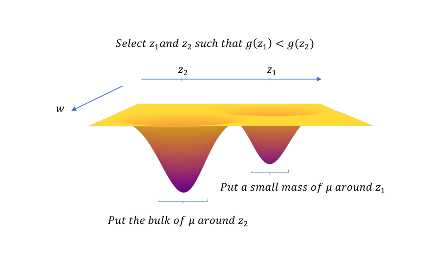
The rigorous proof of 3 requires careful manipulations of different quantities, but the intuition is rather simple. Fig. 3 illustrates the main idea of the proof. We construct a distribution with the majority of the probability mass concentrated around a point where the value of is not minimal. Consequently, for sufficiently small , the distribution of the retained samples will significantly differ from the original distribution. This shift in data distributions causes the algorithm to be non-valid. We see in the next section how we can solve this issue via randomization. Finally, notice that Eq. H1 is generally satisfied in practice since usually for two different examples and in the datasets, the global minimizers of and are different.
4 Solving non-consistency via randomization
We have seen in Section 3 that SBPA algorithms inherently transform the data distribution by asymptotically rejecting all samples in . These algorithms are prone to inconsistency; the transformation of the data distribution translates to a distortion of the loss landscape, potentially leading to a deterioration of the generalization error. This effect is exacerbated for smaller compression ratios as the acceptance region becomes arbitrarily small and concentrated.
With this in mind, one can design practical solutions to mitigate the problem. For illustration, we propose to resort to a Calibration Protocol to retain information from the previously discarded region The calibration protocols can be thought of as wrapper modules that can be applied on top of any SBPA algorithm to solve the consistency issue through randomization (see Fig. 4 for a graphical illustration). Specifically, we split the data budget into two parts: the first part, allocated for the signal, leverages the knowledge from the SBPA and its score function . The second part, allocated for exploration, accounts for the discarded region and consists of a subset of the rejected points, selected uniformly at random. In other words, we write With standard SBPA procedures, We define the proportion of signal in the overall budget. Accordingly, the set of retained points can be expressed as
where denotes the calibrated version of , and the indices ‘s’ and ‘e’ refer to signal and exploration respectively. In this work, we consider the simplest approach. The “signal subset" is composed of the points with the highest importance according to , i.e. . The “exploration subset", is composed on average of points selected uniformly at random from the remaining samples , each sample being retained with probability , independently. The calibrated loss is then defined as a weighted sum of the contributions of the signal and exploration budgets,
| (8) |
where for and The weights and are chosen so that the calibrated procedure is consistent; they are inversely proportional to the probability of acceptance within each region:
4 hereafter states that any SBPA calibrated with this procedure is made consistent as long as a non-zero budget is allocated to exploration. For this reason, we refer to this method as the Exact Calibration protocol (EC). The proof builds on an adapted version of the law of large numbers for sequences of dependent variables which we prove in the Appendix (7).
Proposition 4 (Consistency of Exact Calibration+SBPA)
Let be a SBPA algorithm. Using the Exact Calibration protocol with signal proportion , the calibrated algorithm is consistent if , i.e. the exploration budget is not null. Besides, under the same assumption , the calibrated loss is an unbiased estimator of the generalization loss at any finite sample size ,
The proposed EC protocol offers a simple yet effective approach to address the challenges of non-consistency and non-validity. It can be seamlessly applied in conjunction with any SBPA. The core concept revolves around the implementation of soft-pruning: any data point is assigned a non-zero selection probability. Samples with lower scores are given a higher acceptance rate. The contribution of each accepted data point to the loss is then weighted accordingly. The EC protocol embodies one specific implementation of soft-pruning, offering the advantage of a single interpretable tuning parameter, the signal proportion . By setting to 1 or 0, one can recover the SBPA and Random pruning as extreme cases.
4 states that any SBPA calibrated with EC is made consistent and valid as long as some budget is allocated to exploration. This is empirically validated in Section 5 where we show promising results on a Toy example (Logistic regression) and other image tasks. However, the exact calibration protocol does not systematically allow to outperform random pruning.
Besides, it is worth noting that different implementations of the same general recipe can be considered. It is reasonable to expect that more tailored protocols can be designed to suit specific pruning algorithms and problems. Nevertheless, addressing these questions falls outside the scope of the present work which focus is to provide a framework to analyse data pruning algorithms, as well as to identify and understand their fundamental limitations. We propose the EC protocol to illustrate how this understanding allows to design simple yet efficient solutions to address these limitations.
5 Experiments
5.1 Logistic regression:
We illustrate the main results of this work on a logistic regression task. We consider the following data-generating process
where , and are respectively the uniform and Bernoulli distributions. The class of models is given by
where . We train the models using stochastic gradient descent with the cross entropy loss. For performance analysis, we take and . For the sake of visualization, we take when we plot the loss landscapes (so that the parameter is univariate) and when we plot the data distributions.
We use GraNd (Paul et al., 2021) as a pruning algorithm in a teacher-student setting. For simplicity, we use the optimal model to compute the scores, i.e.
which is proportional to Notice that in this setting, GraNd and EL2N (Paul et al., 2021) are equivalent88 8 This is different from the original version of GraNd , here, we have access to the true generating process, which is not the case in practice.. We bring to the reader’s attention that corresponds to Random pruning in our plots. Indeed, we compare models as a function of the data budget . But notice that in the case of Random, for a given , the values of and do not affect the distribution of the accepted datapoints, and this distribution is always the same as the original data distribution, i.e. when .
Distribution shift and performance degradation: In Section 3, we have seen that the pruning algorithm induces a shift in the data distribution (Fig. 5). This alteration is most pronounced when is small; For , the bottom-left part of the space is populated by and the top-right by . Notice that it was the opposite in the original dataset (). This translates into a distortion of the loss landscape and the optimal parameters of the pruned empirical loss becomes different from . Hence, even when a large amount of data is available, the performance gap does not vanish (Fig. 6).
Calibration with the exact protocol: To solve the distribution shift, we resort to the exact protocol with . In other words, of the budget is allocated to exploration. The signal points (top images in Fig. 8) are balanced with the exploration points (bottom images in Fig. 8). Even though there are nine times fewer of them, the importance weights allow to correct the distribution shift, as depicted in Fig. 2 (Introduction): the empirical losses overlap for all values of , even for small values for which the predominant labels are swapped (for example ). Hence, the performance gap vanishes when enough data is available at any compression ratio (Fig. 7).


Impact of the quality of the pruning algorithm: The calibration protocols allow the performance gap to eventually vanish if enough data is provided. However, from a practical point of view, a natural further requirement is that the pruning method should be better than Random, in the sense that for a given finite budget , the error with the pruning algorithm should be lower than the one of Random. We argue that this mostly decided by the quality of the original SBPA and its score function. Let us take a closer look at what happens in the logistic regression case. For a given , denote the most probable label for the input, i.e. if , and otherwise. As explained, in this setting, GraNd is equivalent to using the score function . For a given value of , consider the quantile of . Notice that if and only if
Therefore, the signal acceptance region is the union of two disjoint sets. The first set is composed of all samples that are close to the decision boundary, i.e. samples for which the true conditional probability is close to . The second set is composed of samples that are further away from the decision boundary, but the realized labels need to be the least probable ones (). These two subsets are visible in Figs. 5 and 8 for and even more for . The signal points can be divided into two sets:
- 1.
the set of points close to the boundary line , where the colors match the original configurations (mostly blue points under the line, red points over the line)
- 2.
the set of points far away from the boundary line, for which the colors are swapped (only red under the line, blue over the line).
Hence, the signal subset corresponding to Condition 1 gives valuable insights; it provides finer-grained visibility in the critical region. However, the second subset is unproductive, as it only retains points that are not representative of their region. Calibration allows mitigating the effect of the second subset while preserving the benefits of the first subset; in Fig. 7, we can see that the calibrated GraNd outperforms random pruning (which corresponds to the curve), requiring on average two to three times fewer data to achieve the same generalization error. However, as becomes lower, will eventually fall under , and the first subset becomes empty (for example, in Fig. 8). Therefore, when becomes small, GraNd does not bring valuable information anymore (for this particular setting). In Fig. 9, we compare GraNd and Calibrated GraNd (with the exact protocol) to Random with . We can see that thanks to the calibration protocol, the performance gap will indeed vanish if enough data is available. However, Random pruning outperforms both versions of GraNd at this compression level. This underlines the fact that for high compression levels, (problem-specific) high-quality pruning algorithms and score functions are required. Given the difficulty of the task, we believe that in the high compression regime ( here), one should allocate a larger budget to random exploration (take smaller values of ).
5.2 Scaling laws with neural networks
The distribution shift is the primary cause of the observed alteration in the loss function, resulting in the emergence of new minima. Gradient descent could potentially converge to a bad minimum, in which case the performance is significantly affected. To illustrate this intuition, we report in Fig. 10 the observed scaling laws for three different synthetic datasets. Let , , , and . The datasets are generated as follows:
1. Linear dataset: we first generate a random vector . Then, we generate training samples and test samples with the rule , where is simulated from .
2. NonLinear dataset (Non-linearity): we first generate a random matrix and a random vector . The samples are then generated with the rule , where is simulated from , and is the ReLU activation function. 99 9 The ReLU activation function is given by for . Here, we abuse the notation a bit and write for .
3. NonLinear+Noisy dataset: we first generate a random vector . Then, we generate training samples and test samples with the rule , where is simulated from and is simulated from and ‘sin’ refers to the sine function.
In Fig. 10, we compare the test error of an 3-layers MLP trained on different subsets generated with either Random pruning, or GraNd. As expected, with random pruning, the results are consistent regardless of the compression level as long as the subset size is the same. With GraNd however, the results depend on the difficulty of the dataset. For the linear dataset, it appears that we can indeed beat the power law scaling, provided that we have access to enough data. In contrast, GraNd seems to perform poorly on the nonlinear and noisy datasets in the high compression regime. This is due to the emergence of new local (bad) minima as decreases as evidenced in Fig. 1. Calibrated with the exact protocol, GraNd becomes valid: we can see that at any compression rate, the error converges to its minimum, which was not the case for . Whether calibration protocols can allow data pruning algorithms to beat the power law scaling remains however an open question: further research is needed in this direction. It is also worth noting that for the Nonlinear datasets, the scaling law pattern exhibits multi-phase behavior. For instance, for the Nonlinear+Noisy dataset, we can (visually) identify two phases, each one of which follows a different power law scaling pattern.
5.3 Image recognition
Through our theoretical analysis, we have concluded that SBPA algorithms are generally non-consistent. This effect is most pronounced when the compression level is small. In this case, the loss landscape can be significantly altered due to the change in the data distribution caused by the pruning procedure. Given a SBPA algorithm, we argue that this alteration in distribution will inevitably affect the performance of the model trained on the pruned subset, and for small , Random pruning becomes more effective than the SBPA algorithm.
In the following, we empirically investigate this behaviour. We evaluate the performance of different SBPA algorithms from the literature and confirm our theoretical predictions with empirical evidence. We consider the following SBPA algorithms:
- •
GraNd (Paul et al., 2021): with this method, given a datapoint , the score function is given by , where is the model output and are the model parameters (e.g. the weights in a neural network) at training step , and where the expectation is taken with respect to random initialization. GraNd selects datapoints with the highest average gradient norm (w.r.t to initialization).
- •
Uncertainty (Coleman et al., 2020): in this method, the score function is designed to capture the uncertainty of the model in assigning a classification label to a given datapoint1010 10 Uncertainty is specifically designed to be used for classification tasks. This means that it is not well-suited for other types of tasks, such as regression.. Different metrics can be used to measure this assignment uncertainty. We focus here on the entropy approach in which case the score function is given by where is the model output probability that belongs to class . For instance, in the context of neural networks, we have , where is the training step where data pruning is performed.
- •
DeepFool (Ducoffe and Precioso, 2018): this method is rooted in the idea that in a classification problem, data points that are nearest to the decision boundary are, in principle, the most valuable for the training process. While a closed-form expression of the margin is typically not available, the authors use a heuristic from the literature on adversarial attacks to estimate the distance to the boundary. Specifically, given a datapoint , perturbations are added to the input until the model assigns the perturbed input to a different class. The amount of perturbation required to change the label for each datapoint defines the score function in this case (see (Ducoffe and Precioso, 2018) for more details).
We illustrate the limitations of the SBPA algorithms above for small , and show that random pruning remains a strong baseline in this case. We further evaluate the performance of our calibration protocols and show that the signal parameter can be tuned so that the calibrated SBPA algorithms outperform random pruning for small . We conduct our experiments using the following setup:
- •
Datasets and architectures. Our framework is not constrained by the type of the learning task or the model. However, for our empirical evaluations, we focus on classification tasks with neural network models. We consider two image datasets: CIFAR10 with ResNet18 and CIFAR100 with ResNet34. More datasets and neural architectures are available in our code, which is based on that of Guo et al., 2022. The code to reproduce all our experiments will be soon open-sourced.
- •
Training. We train all models using SGD with a decaying learning rate schedule that was empirically selected following a grid search. This learning rate schedule was also used in Guo et al., 2022. More details are provided in Appendix D.
- •
Selection epoch. The selection of the coreset can be performed at differnt training stages. We consider data pruning at two different training epochs: , and . We found that going beyond epoch (e.g., using a selection epoch of ) has minimal impact on the performance as compared to using a selection epoch of .
- •
Pruning methods. We consider the following data pruning methods: Random, GraNd, DeepFool, Uncertainty. In addition, we consider the pruning methods resulting from applying the proposed exact calibration protocol to a given SBPA algorithm. We use the notation SBPA-CP1 to refer to the resulting method. For instance, DeepFool-CP1 refers to the method resulting from applying (EC) to DeepFool.


Poor performance of SBPA in the high compression regime: Fig. 11 shows the results of the data pruning methods described above with ResNet18 on CIFAR10 and ResNet34 on CIFAR100. As expected, we observe a consistent decline in the performance of the trained model when the compression ratio is small, typically in the region . More importantly, we observe that SBPA methods (GraNd, DeepFool, Uncertaintyin orange) perform consistently worse than Random pruning (in green), confirming our hypothesis. We also observe that amongst the three SBPA methods, DeepFool is generally the best in the region of interest of and competes with random pruning when the subset selection is performed at training epoch . We noticed that in that setting DeepFool is close to random pruning.
Effect of the calibration protocol Our proposed calibration protocol aim to correct the bias by injecting some randomness in the selection process and keeping (on average) only a fraction of the SBPA method. We notice that the calibration protocol applied to different SBPA consistently boosts the performance in the high compression regime, as can be observed in Fig. 11. Fig. 12 shows that the calibrated SBPA perform better than Random pruning for specific choices of . However, the difference is not always significant. Besides, finding the optimal proportion of signal can be difficult in practice.


6 Related work
As we mentioned in the introduction. The topic of coreset selection has been extensively studied in classical machine learning and statistics (Welling, 2009; Chen et al., 2012; Feldman et al., 2011; Huggins et al., 2016; Campbell and Broderick, 2019). These classical approaches were either model-independent or designed for simple models (e.g. linear models). The recent advances in deep learning has motivated the need for new adapted methods for these deep models. Many approaches have been proposed to adapt to the challenges of the deep learning context. We will cover existing methods that are part of our framework (SBPA algorithms) and others that fall under different frameworks (non-SBPA algorithms).
6.1 Score-based methods
These can generally be categorized into four groups:
- 1.
Geometry based methods: these methods are based on some geometric measure in the feature space. The idea is to remove redundant examples in this feature space (examples that similar representations). Examples include Herding ((Chen et al., 2012)) which aims to greedily select examples by ensuring that the centers of the coreset and that of the full dataset are close. A similar idea based on the K-centroids of the input data was used in (Sener and Savarese, 2017; Agarwal et al., 2020; Sinha et al., 2020).
- 2.
Uncertainty based methods: the aim of such methods is to find the most “difficult" examples, defined as the ones for which the model is the least confident. Different uncertainty measures can be used for this purpose, see (Coleman et al., 2019) for more details.
- 3.
Error based methods: the goal is to find the most significant examples defined as the ones that contribute the most to the loss. In Paul et al., 2021, the authors consider the second norm of the gradient as a proxy to find such examples. Indeed, examples with the highest gradient norm tends to affect the loss more significantly (a first order Taylor expansion of the loss function can explain the intuition behind this proxy). This can be thought of as a relaxation of a Lipschitz-constant based pruning algorithm that was recently introduced in Ayed and Hayou, 2022. Another method consider keeping the most forgettable examples defined as those that change the most often from being well classified to being mis-classified during the course of the training (Toneva et al., 2018). Other methods in this direction consider a score function based on the relative contribution of each example to the total loss over all training examples (see Bachem et al., 2015; Munteanu et al., 2018).
- 4.
Decision boundary based: although this can be encapsulated in uncertainty-based methods, the idea behind these methods is more specific. The aim is to find the examples near the decision boundary, the points for which the prediction has the highest variation (e.g. with respect to the input space, Ducoffe and Precioso, 2018; Margatina et al., 2021).
6.2 Non-SBPA methods
Other methods in the literature select the coreset based on other desirable properties. For instance, one could argue that preserving the gradient is an important feature to have in the coreset as it would lead to similar minima (Killamsetty et al., 2021a; Mirzasoleiman et al., 2020). Other work considered the problem of corset selection as a two-stage optimization problem where the subset selection can be seen also as an optimization problem (Killamsetty et al., 2021b; Killamsetty et al., 2021c). Other methods consider conisder the likelihood and its connection with submodular functions in order to select the subset (Kaushal et al., 2021; Kothawade et al., 2021).
It is worth noting that there exist other approaches to data pruning that involve synthesizing a new dataset with smaller size that preserves certain desired properties, often through the brute-force construction of samples that may not necessarily represent the original data. These methods are known as data distillation methods (see e.g. Wang et al., 2018; Zhao et al., 2021; Zhao and Bilen, 2021) However, these methods have significant limitations, including the difficulty of interpreting the synthesized samples and the significant computational cost. The interpretability issue is particularly a these approaches to use in real-world applications, particularly in high-stakes fields such as medicine and financial engineering.
7 Discussion and Limitations
7.1 Extreme scenarios
Our framework provides insights in the case where both and are large. As a result, there are cases where this framework is not applicable. We call these cases extreme scenarios.
Extreme scenario 1: small .
Our asymptotic analysis can provide insights when a sufficient number of samples are available. In the scarce data regime (small ), our theoretical results may not accurately reflect the impact of pruning on the loss function. It is worth noting, however, that this case is generally not of practical interest as there is no benefit to data pruning when the sample size is small.
Extreme scenario 2: large with ).
In this case, the “effective" sample size after pruning is . Therefore, we cannot glean useful information from the asymptotic behavior of in this case. It is also worth noting that the variance of does not vanish in the limit with fixed, and therefore the empirical mean does not converge to the asymptotic mean.
7.2 Asymptotic results:
1 and 2, and the subsequent corollaries are asymptotic results. They essentially reveal the limitations of SBPA for "large enough models". We decided to take this direction to get results that are as general as possible, showing that the discussed limitations will appear in most situations. 1 and 2 apply to any configuration from a large variety of classes of models, SBPAs, generating processes, and loss functions. The theory readily covers realistic architectures illustrated by Corollary 3, 4 and 5 (in the appendix) that cover wide NN, deep neural NN, and convolutional NN with enough filters. However, these limitations could appear for unrealistically large models. We acknowledge this drawback of the proposed theory and address it in two ways. First, we experimentally show that for the usual settings (ResNet on Cifar), we already observe this significant drop in the performance of SBPAs compared to random pruning. This also aligns with other empirical observations (Guo et al., 2022). In addition, we provide 3 to cover the cases where the class of functions is potentially not rich enough; even in that case, for any SBPA, one can find datasets for which the pruning algorithm will fail for small compression ratios. Besides, to our knowledge, the lines of work that allow one to derive explicit bounds for Neural Networks usually require specific and often overly simplistic architectures (typically one hidden layer feed-forward). In our context, we additionally expect similar strong restrictions to be required for the SBPAs and generating processes. This could wrongfully lead practitioners to consider that using a different SBPA or class of models than the one for which one could derive quantitative results would circumvent the limitations.
7.3 Overparameterized Regime
The scenario in which both the number of parameters and the sample size tend to infinity (e.g. with a constant ratio ) holds practical significance. Our framework does not cover this case and we would like to elucidate the main point at which our proof machinery encounters challenges under this scenario. The main issue resides in understanding the asymptotic behaviour of SBPA algorithms in this context, particularly the extension of Proposition 3. While we can establish concentration with constant and growing large, achieving this with both and going to infinity, especially when the underlying model is a neural network, becomes generally intractable. Nonetheless, under certain supplementary assumptions, it remains feasible to demonstrate concentration.
Recall that in Proposition 3, we essentially use a variation of the law of large numbers to show the convergence in the infinite sample size limit (), while (and consequently, ) is fixed. However, in the scenario where both and tend to infinity, the dependency of on complicates matters, rendering the used variation of the LLN inapplicable. An essential condition under such circumstances becomes the convergence of in a certain sense as well, as . For this purpose, a pertinent tool is LLN for Triangular Arrays, which takes the shape of:
Consider a Triangular Array of random variables such that for each , the variables are iid with mean . Then, under some assumptions (bounded second moments) we have
However, note that in our case, the terms are not necessarily independent, and therefore more advanced LLN for trinagular arrays should be proven and used. We leave this for future work.
7.4 Pruning Time Vs Training Time
In some cases, the pruning procedure might be compute-intensive, and requires more resources than the actual training with the full dataset. This is the case when, for instance, the pruning criterion depends on second order geometry (Hessian etc) and/or multiple perturbations of some quantity (DeepFool), or pruning is performed in multi-shot settings (dynamical pruning). In this paper, we considered pruning criteria that can be performed “one shot” and rely on criteria that involve either gradients (GraNd) or network outputs (Uncertainty) or perturbations of the network output (DeepFool). For GraNd and Uncertainty pruning, the pruning time is typically less than the time required for 1 epoch of training. For DeepFool however, the pruning time might be comparable to 10 epochs of training.
References
- Agarwal et al., (2020) Agarwal, S., Arora, H., Anand, S., and Arora, C. (2020). Contextual diversity for active learning. In ECCV, pages 137–153. Springer.
- Aljundi et al., (2019) Aljundi, R., Lin, M., Goujaud, B., and Bengio, Y. (2019). Gradient based sample selection for online continual learning. Advances in neural information processing systems, 32.
- Arkhangel’skiǐ, (2001) Arkhangel’skiǐ, A. V. (2001). Fundamentals of general topology: Problems and exercises. page 123–124.
- Ayed and Hayou, (2022) Ayed, F. and Hayou, S. (2022). The curse of (non)convexity: The case of an optimization-inspired data pruning algorithm. In I Can’t Believe It’s Not Better Workshop: Understanding Deep Learning Through Empirical Falsification.
- Bachem et al., (2015) Bachem, O., Lucic, M., and Krause, A. (2015). Coresets for nonparametric estimation-the case of dp-means. In ICML, pages 209–217. PMLR.
- Campbell and Broderick, (2019) Campbell, T. and Broderick, T. (2019). Automated scalable bayesian inference via hilbert coresets. The Journal of Machine Learning Research, 20(1):551–588.
- Chen et al., (2012) Chen, Y., Welling, M., and Smola, A. (2012). Super-samples from kernel herding. arXiv preprint arXiv:1203.3472.
- Coleman et al., (2019) Coleman, C., Yeh, C., Mussmann, S., Mirzasoleiman, B., Bailis, P., Liang, P., Leskovec, J., and Zaharia, M. (2019). Selection via proxy: Efficient data selection for deep learning. arXiv preprint arXiv:1906.11829.
- Coleman et al., (2020) Coleman, C., Yeh, C., Mussmann, S., Mirzasoleiman, B., Bailis, P., Liang, P., Leskovec, J., and Zaharia, M. (2020). Selection via proxy: Efficient data selection for deep learning. In International Conference on Learning Representations.
- Deimling, (2010) Deimling, K. (2010). Nonlinear functional analysis. Courier Corporation.
- Ducoffe and Precioso, (2018) Ducoffe, M. and Precioso, F. (2018). Adversarial active learning for deep networks: a margin based approach. arXiv preprint arXiv:1802.09841.
- Feldman et al., (2011) Feldman, D., Faulkner, M., and Krause, A. (2011). Scalable training of mixture models via coresets. Advances in neural information processing systems, 24.
- Guo et al., (2022) Guo, C., Zhao, B., and Bai, Y. (2022). Deepcore: A comprehensive library for coreset selection in deep learning. arXiv preprint arXiv:2204.08499.
- Hernandez et al., (2021) Hernandez, D., Kaplan, J., Henighan, T., and McCandlish, S. (2021). Scaling laws for transfer.
- Hestness et al., (2017) Hestness, J., Narang, S., Ardalani, N., Diamos, G., Jun, H., Kianinejad, H., Patwary, M. M. A., Yang, Y., and Zhou, Y. (2017). Deep learning scaling is predictable, empirically.
- Hoffmann et al., (2022) Hoffmann, J., Borgeaud, S., Mensch, A., Buchatskaya, E., Cai, T., Rutherford, E., de las Casas, D., Hendricks, L. A., Welbl, J., Clark, A., Hennigan, T., Noland, E., Millican, K., van den Driessche, G., Damoc, B., Guy, A., Osindero, S., Simonyan, K., Elsen, E., Vinyals, O., Rae, J. W., and Sifre, L. (2022). An empirical analysis of compute-optimal large language model training. In Oh, A. H., Agarwal, A., Belgrave, D., and Cho, K., editors, Advances in Neural Information Processing Systems.
- Hornik, (1991) Hornik, K. (1991). Approximation capabilities of multilayer feedforward networks. Neural Networks, 4(2):251–257.
- Huggins et al., (2016) Huggins, J., Campbell, T., and Broderick, T. (2016). Coresets for scalable bayesian logistic regression. Advances in Neural Information Processing Systems, 29.
- Kaplan et al., (2020) Kaplan, J., McCandlish, S., Henighan, T., Brown, T. B., Chess, B., Child, R., Gray, S., Radford, A., Wu, J., and Amodei, D. (2020). Scaling laws for neural language models.
- Kaushal et al., (2021) Kaushal, V., Kothawade, S., Ramakrishnan, G., Bilmes, J., and Iyer, R. (2021). Prism: A unified framework of parameterized submodular information measures for targeted data subset selection and summarization. arXiv preprint arXiv:2103.00128.
- Kidger and Lyons, (2020) Kidger, P. and Lyons, T. (2020). Universal approximation with deep narrow networks. In Conference on learning theory, pages 2306–2327. PMLR.
- (22) Killamsetty, K., Durga, S., Ramakrishnan, G., De, A., and Iyer, R. (2021a). Grad-match: Gradient matching based data subset selection for efficient deep model training. In ICML, pages 5464–5474.
- (23) Killamsetty, K., Sivasubramanian, D., Ramakrishnan, G., and Iyer, R. (2021b). Glister: Generalization based data subset selection for efficient and robust learning. In Proceedings of the AAAI Conference on Artificial Intelligence.
- (24) Killamsetty, K., Zhao, X., Chen, F., and Iyer, R. (2021c). Retrieve: Coreset selection for efficient and robust semi-supervised learning. arXiv preprint arXiv:2106.07760.
- Kingma and Ba, (2014) Kingma, D. P. and Ba, J. (2014). Adam: A method for stochastic optimization. arXiv preprint arXiv:1412.6980.
- Kothawade et al., (2021) Kothawade, S., Beck, N., Killamsetty, K., and Iyer, R. (2021). Similar: Submodular information measures based active learning in realistic scenarios. arXiv preprint arXiv:2107.00717.
- Margatina et al., (2021) Margatina, K., Vernikos, G., Barrault, L., and Aletras, N. (2021). Active learning by acquiring contrastive examples. arXiv preprint arXiv:2109.03764.
- Mirzasoleiman et al., (2020) Mirzasoleiman, B., Bilmes, J., and Leskovec, J. (2020). Coresets for data-efficient training of machine learning models. In ICML. PMLR.
- Munteanu et al., (2018) Munteanu, A., Schwiegelshohn, C., Sohler, C., and Woodruff, D. P. (2018). On coresets for logistic regression. In NeurIPS.
- Paul et al., (2021) Paul, M., Ganguli, S., and Dziugaite, G. K. (2021). Deep learning on a data diet: Finding important examples early in training.
- Robbins and Monro, (1951) Robbins, H. and Monro, S. (1951). A stochastic approximation method. The annals of mathematical statistics, pages 400–407.
- Rosenfeld et al., (2020) Rosenfeld, J. S., Rosenfeld, A., Belinkov, Y., and Shavit, N. (2020). A constructive prediction of the generalization error across scales. In International Conference on Learning Representations.
- Sener and Savarese, (2017) Sener, O. and Savarese, S. (2017). Active learning for convolutional neural networks: A core-set approach. arXiv preprint arXiv:1708.00489.
- Sinha et al., (2020) Sinha, S., Zhang, H., Goyal, A., Bengio, Y., Larochelle, H., and Odena, A. (2020). Small-gan: Speeding up gan training using core-sets. In ICML. PMLR.
- Sorscher et al., (2022) Sorscher, B., Geirhos, R., Shekhar, S., Ganguli, S., and Morcos, A. S. (2022). Beyond neural scaling laws: beating power law scaling via data pruning. In Oh, A. H., Agarwal, A., Belgrave, D., and Cho, K., editors, Advances in Neural Information Processing Systems.
- Toneva et al., (2018) Toneva, M., Sordoni, A., Combes, R. T. d., Trischler, A., Bengio, Y., and Gordon, G. J. (2018). An empirical study of example forgetting during deep neural network learning. arXiv preprint arXiv:1812.05159.
- Varadarajan, (1958) Varadarajan, V. S. (1958). On the convergence of sample probability distributions. Sankhyā: The Indian Journal of Statistics (1933-1960), 19(1/2):23–26.
- Wang et al., (2018) Wang, T., Zhu, J.-Y., Torralba, A., and Efros, A. A. (2018). Dataset distillation. arXiv preprint arXiv:1811.10959.
- Welling, (2009) Welling, M. (2009). Herding dynamical weights to learn. In Proceedings of the 26th Annual International Conference on Machine Learning, pages 1121–1128.
- Zhai et al., (2022) Zhai, X., Kolesnikov, A., Houlsby, N., and Beyer, L. (2022). Scaling vision transformers. In Proceedings of the IEEE/CVF Conference on Computer Vision and Pattern Recognition (CVPR), pages 12104–12113.
- Zhao and Bilen, (2021) Zhao, B. and Bilen, H. (2021). Dataset condensation with differentiable siamese augmentation. In International Conference on Machine Learning.
- Zhao et al., (2021) Zhao, B., Mopuri, K. R., and Bilen, H. (2021). Dataset condensation with gradient matching. In International Conference on Learning Representations.
- Zhou, (2020) Zhou, D.-X. (2020). Universality of deep convolutional neural networks. Applied and computational harmonic analysis, 48(2):787–794.
8 Acknowledgement
We would like to thank the authors of DeepCore project (Guo et al., 2022) for open-sourcing their excellent code1111 11 The code by Guo et al., 2022 is available at https://github.com/PatrickZH/DeepCore.. The high flexibility and modularity of their code allowed us to quickly implement our calibration protocols on top of existing SBPA algorithms.
Appendix A Proofs
A.1 Proofs of Section 2
Lemma 1
Let be a distribution on and a sequence of parameters in satisfying
Then, it comes that
Proof:
Denote the function from to defined by
Notice that under our assumptions, the dominated convergence theorem gives that is continuous. This lemma is a simple consequence of the continuity of and the compacity of . Consider a sequence such that
We can prove the lemma by contradiction. Consider and assume that there exists infinitely many indices for which Since is compact, we can assume that is convergent (by considering a subsequence of which if needed), denote its limit. The continuity of then gives that , and in particular
But since is continuous, the initial assumption on translates to
concluding the proof.
Proposition 1. A pruning algorithm is valid at a compression ratio if and only if
where and denotes the euclidean distance from the point to the set .
Proof:
Proof:
Leveraging Lemma 1, it is enough to prove that
To simplify the notations, we introduce the function from to defined by
where Since is compact, we can find such that . It comes that
The last term converges to zero almost surely by assumption. By definition of , the middle term is non-positive. It remains to show that the first term also converges to zero. With this, we can conclude that
To prove that the first term converges to zero, we use the classical result that if every subsequence of a sequence has a further subsequence that converges to , then the sequence converges to . Denote
By compacity of , from any subsequence of we can extract a further subsequence with indices denoted such that converges to some . We will show that converges to . Let , since is continuous on the compact set , it is uniformly continuous. Therefore, almost surely, for large enough,
Denoting
the triangular inequality then gives that, almost surely, for large enough
By assumption, the sequence converges to zero almost surely, which concludes the proof.
We now prove Corollary 2, since Corollary 1 is a straightforward application of 2.
Proof:
This proposition is a direct consequence of 2 that states that
Since the is continuous on the compact , it is uniformly continuous. Hence, for any , we can find such that if , then for any parameters . Hence, for large enough, , leading to
Since the algorithm is valid, we know that converges to almost surely. Therefore, for any ,
which concludes the proof.
A.2 Proof of 3
Proposition 3. [Asymptotic behavior of SBPA]
Let be a SBPA algorithm and let be its corresponding score function. Assume that is adapted, and consider a compression ratio . Denote by the quantile of the random variable where . Denote . Almost surely, the empirical measure of the retained data samples converges weakly to ,
where is the restriction of to the set . In particular, we have that
Proof:
Consider the set of functions that are continuous. We will show that
| (9) |
To simplify the notations, and since converges to 1, we will assume that is an integer. Denote the ordered statistic of , and the quantile of the random variable where .
We can upper bound the left hand side in equation (9) by the sum of two random terms and defined by
To conclude the proof, we will show that both terms converge to zero almost surely.
For any , denoting the empirical cumulative density function (cdf) of and the cdf of , we have that
Therefore, which converges to zero almost surely by the Glivenko-Cantelli theorem.
Similarly, the general Glivenko-Cantelli theorem for metric spaces (Varadarajan, 1958) gives that almost surely,
Consider . Since is continuous and is compact, the sets and are disjoint and closed subsets. Using Urysohn’s lemma (Theorem 8 in the Appendix), we can find such that if and if . Consider , it comes that
Hence, noticing that , we find that
We can conclude the proof by noticing that converges to and taking .
A.3 Proof of 1
In order to prove the theorem, we will need a few technical results that we state and prove first.
Lemma 2
Consider a set of continuous functions from to . Consider a function in the closure of for the norm. Then for any , there exists such that
Proof:
Since the loss is continuous on the compact , it is uniformly continuous. We can therefore find such that for any , if then We conclude the proof using by selecting any that is at a distance not larger than from for the norm.
Lemma 3
Consider a SBPA . Let be a set of continuous functions from to . Consider and assume that is consistent on at level , i.e.
Let be any measurable function from to . If there exists a sequence of elements of that converges point-wise to , then
| (10) |
In particular, if has the universal approximation property, then (10) holds for any continuous function.
Proof:
Le be a sequence of functions in that converges point-wise to . Consider , since is consistent and that is continuous and bounded, 3 gives that
Since is bounded, we can apply the dominated convergence theorem to both sides of the equation to get the final result.
5 hereafter proves the final result for SBPA that do not depend on the labels. The proof of 1 that follows essentially deals with the remaining case of SBPA that depend on the labels.
Proposition 5
Let be any SBPA with an adapted score function satisfying
Assume that there exists two continuous functions and such that
If has the universal approximation property, then there exist hyper-parameters for which the algorithm is not consistent.
Proof:
Consider a compression ratio . We will prove the result by means of contradiction. Assume that the SBPA is consistent on . From the universal approximation property and Lemma 3, we get that
from which we deduce that
| (11) | |||||
| (12) |
and similarly for .
Notice that since the score function does not depend on , there exists such that . Consider the function defined by
we will show that
- i)
- ii)
There exists a sequence of elements in that converges point-wise almost everywhere to
The conjunction of these two points contradicts Lemma 3, which would conclude the proof.
The first point is obtained through simple derivations, evaluating both sides of the equation i).
where we successively used the definition of and equation (11). Now, using the definition of , we get that
These derivations lead to
by assumption on and .
For point ii), we will construct a sequence of functions in that converges point-wise to almost everywhere, using the definition of the universal approximation property and Urysohn’s lemma (Lemma 8 in the Appendix). Consider and denote . Denote and the and quantile of the random variable where . Denote and . Since is continuous and is compact, the two sets are closed. Besides, since the random variable is continuous ( is an adapted score function), both sets are disjoint. Therefore, using Urysohn’s lemma (Lemma 8 in the Appendix), we can chose a continuous function such that for and for . Denote the function defined by
Notice that converges point-wise to , and therefore converges point-wise to . Besides, since is continuous, and has the universal approximation property, we can chose such that
Hence, for any input , we can upper-bound by , giving that converges pointwise to and concluding the proof.
We are now ready to prove the 1 that we state here for convenience.
Theorem 1. Let be any SBPA algorithm with an adapted score function. If has the universal approximation property, then there exist hyper-parameters for which the algorithm is not consistent.
Proof:
We will use the universal approximation theorem to construct a model for which the algorithm is biased. Denote the support of the generating measure . We can assume that there exists such that , , and otherwise one can apply 5 to get the result. Denote such that . Since is continuous, we can find such that
| (13) |
where is the quantile of where .
Since , it comes that
By assumption, the distribution of is dominated by the Lebesgue measure, we can therefore find a positive such that
The sets and are closed and disjoint sets, Lemma 8 in Appendix insures the existance of a continuous function such that for , and for . We use Lemma 2 to construct such that for any , Let and . Denote . Notice that if we assume that the algorithm is consistent on , Lemma 3 gives that We will prove the non-consistency result by means of contradiction, showing that instead we have
| (14) |
To do so, we start by noticing three simple results that are going to be used in the following derivations
- •
,
- •
, and
- •
A.4 Proof of 2
Denote the set of probability distributions on , such that the marginal distribution on the input space is continuous (absolutely continuous with respect to the Lebesgue measure on ) and for which
is upper semi-continuous. For a probability measure , denote the marginal distribution on the input. Denote the function from to defined by
Finally, denote the set of continuous functions from to . We recall the two assumptions made on the loss:
- (i)
The loss is non-negative and that if and only if
- (ii)
For , has a unique minimizer, denoted , that is increasing with .
Lemma 4
Consider a loss that satisfies (ii). Then, for any and , there exists such that for any
Proof:
Consider and . Assume that for any there exists such that and
Since is compact, we can assume that the sequence converges (taking, if needed, a sub-sequence of the original one). Denote this limit. Since and are continuous, it comes that and
contradicting the assumption that is unique.
Lemma 5
If is a measurable map from to , then there exists a sequence of continuous functions that converges point-wise to (for the Lebesgue measure)
Proof:
This result is a direct consequence of two technical results, the Lusin’s Theorem (5 in the appendix), and the continuous extension of functions from a compact set (6 in the appendix).
Lemma 6
For a distribution . define the function from to by
is measurable. Besides,
Proof:
The function from to defined by
is well defined and increasing from assumption (ii) on the loss. It is, therefore, measurable. Since is measurable, we get that is measurable as the composition of two measurable functions. For the second point, notice that by definition of , for any ,
Using Lemma 5, we can take a sequence of continuous functions that converge point-wise to . We can conclude using the dominated convergence theorem, leveraging that is bounded.
Lemma 7
Let a SBPA with an adapted score function that depends on the labels. Then there exists a compression level and such that for any , the two following statements exclude each other
- (i)
- (ii)
Proof:
Since depends on the labels, we can find in the support of such that and . Without loss of generality, we can assume that . Take such that
By continuity of , we can find a radius such that for any in the ball of center and radius , we have that . Besides, since is upper semi-continuous, we can assume that is small enough to ensure that for any ,
| (15) |
Therefore, recalling that
- •
and
- •
and
Denote Consider the subset defined by
We can derive a lower-bound on as follows:
The last inequality gives that . Moreover, we can lower-bound using (15) as follows:
Therefore, assumptions i) and ii) on the loss give that and for any . Using Lemma 4, take such that
| (16) |
In the following, we will show that there exists such that for any ,
| (17) |
Otherwise, leveraging the compacity of the sets at hand, we can find two converging sequences and such that
Since is uniformly continuous,
is continuous. Taking the limit it comes that
and consequently . Since ,
reaching a contradiction.
Now, take and satisfying (16) and (17) respectively. Put together, we have that for any ,
Using the definition of , it comes that for any function and
| (18) |
Let . Consider satisfying
We will prove that
to conclude the proof. Denote is the subset of such that for any , We get that
Hence we get that . Since the right hand side of (18) holds. In other words,
from which we successively obtain
We can now ready to prove 2.
Theorem 2. Let a SBPA with an adapted score function that depends on the labels. If has the universal approximation property and the loss satisfies assumptions (i) and (ii), then there exist two hyper-parameters such that the algorithm is not valid on .
Proof:
Denote , and for , and . We will leverage 1 and Lemma 7 show that there exist a compression ratio and a hyper-parameter such that
which would conclude the proof.
Using Lemma 7, we can find and such that for any continuous function , the two following propositions exclude each other:
- (i)
- (ii)
Since has the universal approximation property, and that and (defined as in Lemma 6) are measurable, we consecutively use Lemma 5 and Lemma 2 to find such that
- 1.
There exists such that
- 2.
There exists such that
Take two such functions. Consider any parameter By definition, it comes that
Therefore, since Lemma 6 gives that , we can conclude that
from which we deduce that
which gives the desired result.
A.5 Proof of the Corollaries 3 and 4
These two corollaries are a straightforward application of 1 and 2 as well as the existing literature on the universal approximation properties of Neural Networks: (Hornik, 1991) and (Kidger and Lyons, 2020). We give the proof of the result for wide neural networks. Consider any number of hidden layers fixed. Denote . (Hornik, 1991) implies that has the universal approximation property. 1 states that one can find a such that the SBPA is not consistent on . Now from the definition of consistency, we get that if a SBPA is not consistent on , then it is not consistent on any superset that contains . Therefore, we get the non-consistency result by noticing that
for any and . Similarly, 2 states that there exist and such that the model is not valid for any class of model such that
We can conclude noticing that satisfies this condition if and .
A.6 Proof of 3
For , denote the set of generating processes for -classes classification problems, for which the input is a continuous random variable (the marginal of the input is dominated by the Lebesgue measure), and the output can take one of values in (the same for all ). Similarly, denote , the set of generating processes for regression problems for which both the input and output distributions are continuous. Let be any set of generating processes introduced previously for regression or classification (either for some , or ).
Assume that there exist such that
| (H1) |
For any SBPA algorithm with adapted criterion, we will show that there exists a generating process for which is not valid. More precisely, we will show that there exists such that for any compression ratio , there exists a generating process for which is not valid. To do so, we leverage Corollary 2 and prove that for any , there exists , for which , i.e.
| (19) |
We bring to the reader’s attention that depends on , and so does the acceptance region .
The rigorous proof of 3 requires careful manipulations of different quantities, but the idea is rather simple. Fig. 13 illustrates the main idea of the proof. We construct a distribution with the majority of the probability mass concentrated around a point where the value of is not minimal.
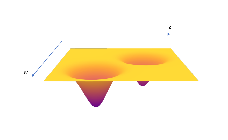

We start by introducing further notations. For , and , we denote by the function defined by We will use the generic notation to refer to the Euclidean norm on the appropriate space. We denote the ball with center and radius . If is a set, then For , we denote
Notice that is continuous on Besides, the set data generating processes is i) convex and ii) satisfies for all , and , there exists a probability measure such that
These conditions play a central role in the construction of a generating process for which the pruning algorithm is not valid. In fact, the non-validity proof applies to any set of generating processes satisfying conditions i) and ii). To ease the reading of the proof, we break it into multiple steps that we list hereafter.
Steps of the proof:
- 1.
For all , the set is compact (and non empty).
- 2.
For all , there exists such that for all ,
- 3.
Under assumption (H1), there exists such that i) and ii)
- 4.
For as in 3, denote and . There exists such that for any and and
- 5.
For any , there exits a generating process such that any minimizer of the pruned program necessarily satisfies and such that for a given .
- 6.
such that , such that for any
Proof:
Result 1: Let . Since is compact and functions is continuous, it comes that is well defined, non-empty and closed (as the inverse image of a closed set). Hence it is compact.
Result 2: Let and . We will prove the result by contradiction. Suppose that for any , there exists such that
It is well known that since is continuous and that is compact, the function
is continuous. Therefore, for any , we can find such that for any ,
For every , let such that , and . By definition, . Since is compact, we can assume that converges to without loss of generality (taking a sub-sequence of the original one). Now, notice that
therefore, since is continuous, and so , which contradicts the fact that for all . Hence, we can find such that for all .
Result 3: Let as in (H1) such that . Since is continuous, and and are compact, is also compact. Hence, there exists such that
Using the previous result, let such that The triangular inequality yields . Since is adapted and has strictly positive Lebesgue measure, we can find such that . Therefore, the points satisfy the requirements.
Result 4: Since is compact and is continuous, is compact, and since ,
for any . Denote .
Since is continuous on the compact space , it is uniformly continuous. We can hence take such that for and such that
Using Result 2, we can find such that for all ,
We can assume without loss of generality that . Let . For any , we conclude that
Result 5: Let defined previously, and . Using the uniform continuity of , we construct such that
Consider such that and . Let . It comes that Using a proof by contradiction, we will show that there exists such that
Suppose that the result doesn’t hold, we can define a sequence of minimizers such that and Denote Take any
| (20) | |||||
| (21) | |||||
| (22) | |||||
| (23) |
Similarly, we have that
| (24) | |||||
| (25) | |||||
| (26) |
Putting the two inequalities together, we find
Since is compact, we can assume that (taking a sub-sequence of the original one). And since is continuous, we can deduce that , which contradict the fact that for all .
Result 6: Let and as in the previous results. Let From Result 5, we have that For , Result 5 implies that
Therefore,
| (27) | |||||
| (28) | |||||
| (29) | |||||
| (30) |
Therefore,
which is strictly positive for
A.7 Proof of 4
Proposition 4. [Consistency of Exact Calibration+SBPA]
Let be a SBPA algorithm. Using the Exact Calibration protocol with signal proportion , the calibrated algorithm is consistent if , i.e. the exploration budget is not null. Besides, under the same assumption , the calibrated loss is an unbiased estimator of the generalization loss at any finite sample size ,
Proof:
Consider . Let , and . For , consider the independent Bernoulli random variables . Notice that
which gives
Define the random variables
Let be the -algebra generated by the random variables . Let us now show that the conditions of 7 hold with this choice of .
- •
Let and . Similarly to the previous computation, we get that .
- •
Using the compactness assumption on the space and , we trivially have that .
- •
Trivially, for each , the variables are identically distributed.
Using 7 and the standard strong law of large numbers, we have that almost surely, and almost surely, which concludes the proof for the consistency.
Appendix B Technical results
Theorem 4 (Universal Approximation Theorem, (Hornik, 1991))
Let denote the set of continuous functions from to . Let . Then, is not polynomial if and only if for every , compact , , , there exist , , , such that
where
Lemma 8 (Urysohn’s lemma, (Arkhangel’skiǐ, 2001))
For any two disjoint closed sets and of a topological space , there exists a real-valued function , continuous at all points, taking the value at all points of , the value at all points of . Moreover, for all , .
Theorem 5 (Lusin’s Theorem)
If is a topological measure space endowed with a regular measure , if is second-countable and is measurable, then for every there exists a compact set such that and the restriction of to is continuous.
Theorem 6 (Continuous extension of functions from a compact, (Deimling, 2010))
Let be compact and be a continuous function. Then there exists a continuous extension such that for all .
B.1 A generalized Law of Large Numbers
There are many extensions of the strong law of large numbers to the case where the random variables have some form of dependence. We prove a strong law of large numbers for specific sequences of arrays that satisfy a conditional zero-mean property.
Theorem 7
Let be a triangular array of random variables satisfying the following conditions:
- •
For all and , , where , i.e. the -algebra generated by all the random variables in row other than .
- •
For all , the random variables are identically distributed (but not necessarily independent).
- •
.
Then, we have that
Proof:
The proof uses similar techniques to the standard proof of the strong law of large numbers, with some key differences, notably in the use of the Chebychev inequality to upper-bound the fourth moment of the mean. Let . We want to show that . This is equivalent to showing that for all , . This event is nothing but the limsup of the events . Hence, we can use Borel-Cantelli to conclude if we can show that .
Let . Using Chebychev inequality with degree , we have that . It remains to bound to conclude. We have that . Using the first condition (zero-mean conditional distribution), all the terms of the form , , and for vanish and we end up with , where we have used the fact that the number of terms of the form in the sum is given by . Using the last condition of the fourth moment, we obtain that there exists a constant such that . Using Chebychev inequality, we get that , and thus . We conclude using the Borel-Cantelli lemma.
Appendix C Additional Theoretical Results
Convolutional neural networks: For an activation function , a real number , and integers and denote the set of convolutional neural networks with filters of length , with all weights and biases in . More precisely, for a filter mask , and a vector , the results of the convolution of and , denoted is a vector in defined by A network from is then defined recursively for :
- •
- •
For , , where the filters and biases and are in
- •
, where the vector has entries in
Corollary 5 (Convolutional Neural Networks (Zhou, 2020))
Let be the ReLU activation function. Consider a filter length For any SBPA with adapted score function, there exists a number of filters and a radius such that the algorithm is not consistent on , for any and . Besides, if the algorithm depends on the labels, then it is also not valid on , for any and .
Appendix D Experimental details
| Dataset | CIFAR10 | CIFAR100 |
|---|---|---|
| Architecture | ResNet18 | ResNet34 |
| Methods | GraNd(10), Uncertainty, DeepFool | GraNd(10), Uncertainty, DeepFool |
| Selection LR | 0.1 | 0.1 |
| Training LR | 0.1 | 0.1 |
| Selection Epochs | 1, 5 | 1, 5 |
| Nb of exps | 3 | 3 |
| Training Epochs | 160 | 160 |
| Optimizer | SGD | SGD |
| Batch Size | 128 | 128 |
The table above contains the different hyper-parameter we used to run the experiments. GraNd(10) refers to using the GraNd method with different seeds (averaging over 10 different initializations). Selection LR refers to the learning rate used for the coreset selection. The training LR follwos a cosine annealing schedule given by the following:
where is the current epoch, is the total number of epochs, and and . These are the same hyper-parameter choices used by Guo et al., 2022.
D.1 MLP for Scaling laws experiments
We consider an MLP given by
where is the input, are the weight matrices and are the bias vectors.