跳到论文正文
W Papers独立论文阅读器 arXiv:2302.06889 论文正文 计算阅读时间 · 0%
引用这篇论文根据当前论文元数据生成,正式投稿前建议核对。


License: arXiv.org perpetual non-exclusive license
arXiv:2302.06889v1 [cs.DS] 14 Feb 2023

Worst Case and Probabilistic Analysis of the 2-Opt Algorithm for the TSPThanks: An extended abstract of this work has appeared in the Proceedings of the 18th ACM-SIAM Symposium on Discrete Algorithms (SODA 2007). The results of this extended abstract have been split into two journal articles [6] and [7]. This report is an updated version of [6], in which two minor errors in the proofs of Lemma 8 and Lemma 9 have been corrected. We thank Bodo Manthey for pointing out these errors. This work was supported in part by the EU within the 6th Framework Programme under contract 001907 (DELIS), by DFG grants VO 889/2 and WE 2842/1, and by EPSRC grant EP/F043333/1. We thank the referee of [6] for her/his extraordinary efforts and many helpful suggestions.

Matthias Englert Thanks: DIMAP and Dept.˜of Computer Science, University of Warwick englert@dcs.warwick.ac.uk    Heiko Röglin Thanks: Dept.˜of Computer Science, University of Bonn roeglin@cs.uni-bonn.de    Berthold Vöcking Thanks: Dept.˜of Computer Science, RWTH Aachen University
Abstract

2-Opt is probably the most basic local search heuristic for the TSP. This heuristic achieves amazingly good results on “real world” Euclidean instances both with respect to running time and approximation ratio. There are numerous experimental studies on the performance of 2-Opt. However, the theoretical knowledge about this heuristic is still very limited. Not even its worst case running time on 2-dimensional Euclidean instances was known so far. We clarify this issue by presenting, for every p∈ℕp\in\mathbb{N}, a family of LpL_{p} instances on which 2-Opt can take an exponential number of steps.

Previous probabilistic analyses were restricted to instances in which nn points are placed uniformly at random in the unit square [0,1]2[0,1]^{2}, where it was shown that the expected number of steps is bounded by O~​(n10)\tilde{O}(n^{10}) for Euclidean instances. We consider a more advanced model of probabilistic instances in which the points can be placed independently according to general distributions on [0,1]d[0,1]^{d}, for an arbitrary d≥2d\geq 2. In particular, we allow different distributions for different points. We study the expected number of local improvements in terms of the number nn of points and the maximal density ϕ\phi of the probability distributions. We show an upper bound on the expected length of any 2-Opt improvement path of O~​(n4+1/3⋅ϕ8/3)\tilde{O}(n^{4+1/3}\cdot\phi^{8/3}). When starting with an initial tour computed by an insertion heuristic, the upper bound on the expected number of steps improves even to O~​(n4+1/3−1/d⋅ϕ8/3)\tilde{O}(n^{4+1/3-1/d}\cdot\phi^{8/3}). If the distances are measured according to the Manhattan metric, then the expected number of steps is bounded by O~​(n4−1/d⋅ϕ)\tilde{O}(n^{4-1/d}\cdot\phi). In addition, we prove an upper bound of O⁡(ϕd)O(\sqrt[d]{\phi}) on the expected approximation factor with respect to all LpL_{p} metrics.

Let us remark that our probabilistic analysis covers as special cases the uniform input model with ϕ=1\phi=1 and a smoothed analysis with Gaussian perturbations of standard deviation σ\sigma with ϕ∼1/σd\phi\sim 1/\sigma^{d}.

1 Introduction

In the traveling salesperson problem (TSP), we are given a set of vertices and for each pair of distinct vertices a distance. The goal is to find a tour of minimum length that visits every vertex exactly once and returns to the initial vertex at the end. Despite many theoretical analyses and experimental evaluations of the TSP, there is still a considerable gap between the theoretical results and the experimental observations. One important special case is the Euclidean TSP in which the vertices are points in ℝd\mathbb{R}^{d}, for some d∈ℕd\in\mathbb{N}, and the distances are measured according to the Euclidean metric. This special case is known to be NP-hard in the strong sense [17], but it admits a polynomial time approximation scheme (PTAS), shown independently in 1996 by Arora [1] and Mitchell [15]. These approximation schemes are based on dynamic programming. However, the most successful algorithms on practical instances rely on the principle of local search and very little is known about their complexity.

The 2-Opt algorithm is probably the most basic local search heuristic for the TSP. 2-Opt starts with an arbitrary initial tour and incrementally improves this tour by making successive improvements that exchange two of the edges in the tour with two other edges. More precisely, in each improving step the 22-Opt algorithm selects two edges {u1,u2}\{u_{1},u_{2}\} and {v1,v2}\{v_{1},v_{2}\} from the tour such that u1,u2,v1,v2u_{1},u_{2},v_{1},v_{2} are distinct and appear in this order in the tour, and it replaces these edges by the edges {u1,v1}\{u_{1},v_{1}\} and {u2,v2}\{u_{2},v_{2}\}, provided that this change decreases the length of the tour. The algorithm terminates in a local optimum in which no further improving step is possible. We use the term 2-change to denote a local improvement made by 2-Opt. This simple heuristic performs amazingly well on “real-life” Euclidean instances like, e.g., the ones in the well-known TSPLIB [19]. Usually the 2-Opt heuristic needs a clearly subquadratic number of improving steps until it reaches a local optimum and the computed solution is within a few percentage points of the global optimum [9].

There are numerous experimental studies on the performance of 2-Opt. However, the theoretical knowledge about this heuristic is still very limited. Let us first discuss the number of local improvement steps made by 2-Opt before it finds a locally optimal solution. When talking about the number of local improvements, it is convenient to consider the state graph. The vertices in this graph correspond to the possible tours and an arc from a vertex vv to a vertex uu is contained if uu is obtained from vv by performing an improving 2-Opt step. On the positive side, van Leeuwen and Schoone consider a 2-Opt variant for the Euclidean plane in which only steps are allowed that remove a crossing from the tour. Such steps can introduce new crossings, but van Leeuwen and Schoone [22] show that after O⁡(n3)O(n^{3}) steps, 2-Opt finds a tour without any crossing. On the negative side, Lueker [14] constructs TSP instances whose state graphs contain exponentially long paths. Hence, 2-Opt can take an exponential number of steps before it finds a locally optimal solution. This result is generalized to kk-Opt, for arbitrary k≥2k\geq 2, by Chandra, Karloff, and Tovey [3]. These negative results, however, use arbitrary graphs that cannot be embedded into low-dimensional Euclidean space. Hence, they leave open the question as to whether it is possible to construct Euclidean TSP instances on which 2-Opt can take an exponential number of steps, which has explicitly been asked by Chandra, Karloff, and Tovey. We resolve this question by constructing such instances in the Euclidean plane. In chip design applications, often TSP instances arise in which the distances are measured according to the Manhattan metric. Also for this metric and for every other LpL_{p} metric, we construct instances with exponentially long paths in the 2-Opt state graph.

Theorem 1.

For every p∈{1,2,3,…}∪{∞}p\in\{1,2,3,\ldots\}\cup\{\infty\} and n∈ℕ={1,2,3,…}n\in\mathbb{N}=\{1,2,3,\ldots\}, there is a two-dimensional TSP instance with 16​n16n vertices in which the distances are measured according to the LpL_{p} metric and whose state graph contains a path of length 2n+4−222^{n+4}-22.

For Euclidean instances in which nn points are placed independently uniformly at random in the unit square, Kern [10] shows that the length of the longest path in the state graph is bounded by O⁡(n16)O(n^{16}) with probability at least 1−c/n1-c/n for some constant cc. Chandra, Karloff, and Tovey [3] improve this result by bounding the expected length of the longest path in the state graph by O⁡(n10​log⁡n)O(n^{10}\log{n}). That is, independent of the initial tour and the choice of the local improvements, the expected number of 2-changes is bounded by O⁡(n10​log⁡n)O(n^{10}\log{n}). For instances in which nn points are placed uniformly at random in the unit square and the distances are measured according to the Manhattan metric, Chandra, Karloff, and Tovey show that the expected length of the longest path in the state graph is bounded by O⁡(n6​log⁡n)O(n^{6}\log{n}).

We consider a more general probabilistic input model and improve the previously known bounds. The probabilistic model underlying our analysis allows different vertices to be placed independently according to different continuous probability distributions in the unit hypercube [0,1]d[0,1]^{d}, for some constant dimension d≥2d\geq 2. The distribution of a vertex viv_{i} is defined by a density function fi:[0,1]d→[0,ϕ]f_{i}\colon[0,1]^{d}\to[0,\phi] for some given ϕ≥1\phi\geq 1. Our upper bounds depend on the number nn of vertices and the upper bound ϕ\phi on the density. We denote instances created by this input model as ϕ\phi-perturbed Euclidean or Manhattan instances, depending on the underlying metric. The parameter ϕ\phi can be seen as a parameter specifying how close the analysis is to a worst case analysis since the larger ϕ\phi is, the better can worst case instances be approximated by the distributions. For ϕ=1\phi=1 and d=2d=2, every point has a uniform distribution over the unit square, and hence the input model equals the uniform model analyzed before. Our results narrow the gap between the subquadratic number of improving steps observed in experiments [9] and the upper bounds from the probabilistic analysis. With slight modifications, this model also covers a smoothed analysis, in which first an adversary specifies the positions of the points and after that each position is slightly perturbed by adding a Gaussian random variable with small standard deviation σ\sigma. In this case, one has to set ϕ=1/(2​π​σ)d\phi=1/(\sqrt{2\pi}\sigma)^{d}.

We prove the following theorem about the expected length of the longest path in the 2-Opt state graph for the three probabilistic input models discussed above. It is assumed that the dimension d≥2d\geq 2 is an arbitrary constant.

Theorem 2.

The expected length of the longest path in the 2-Opt state graph

  1. a)

    is O⁡(n4⋅ϕ)O(n^{4}\cdot\phi) for ϕ\phi-perturbed Manhattan instances with nn points.

  2. b)

    is O⁡(n4+1/3⋅log⁡(n​ϕ)⋅ϕ8/3)O(n^{4+1/3}\cdot\log(n\phi)\cdot\phi^{8/3}) for ϕ\phi-perturbed Euclidean instances with nn points.

Usually, 2-Opt is initialized with a tour computed by some tour construction heuristic. One particular class is that of insertion heuristics, which insert the vertices one after another into the tour. We show that also from a theoretical point of view, using such an insertion heuristic yields a significant improvement for metric TSP instances because the initial tour 2-Opt starts with is much shorter than the longest possible tour. In the following theorem, we summarize our results on the expected number of local improvements.

Theorem 3.

The expected number of steps performed by 2-Opt

  1. a)

    is O⁡(n4−1/d⋅log⁡n⋅ϕ)O(n^{4-1/d}\cdot\log{n}\cdot\phi) on ϕ\phi-perturbed Manhattan instances with nn points when 2-Opt is initialized with a tour obtained by an arbitrary insertion heuristic.

  2. b)

    is O⁡(n4+1/3−1/d⋅log2⁡(n​ϕ)⋅ϕ8/3)O(n^{4+1/3-1/d}\cdot\log^{2}(n\phi)\cdot\phi^{8/3}) on ϕ\phi-perturbed Euclidean instances with nn points when 2-Opt is initialized with a tour obtained by an arbitrary insertion heuristic.

In fact, our analysis shows not only that the expected number of local improvements is polynomially bounded but it also shows that the second moment and hence the variance is bounded polynomially for ϕ\phi-perturbed Manhattan instances. For the Euclidean metric, we cannot bound the variance but the 3/23/2-th moment polynomially.

In [5], we also consider a model in which an arbitrary graph G=(V,E)G=(V,E) is given along with, for each edge e∈Ee\in E, a probability distribution according to which the edge length 𝖽⁡(e)\dist(e) is chosen independently of the other edge lengths. Again, we restrict the choice of distributions to distributions that can be represented by density functions fe:[0,1]→[0,ϕ]f_{e}\colon[0,1]\to[0,\phi] with maximal density at most ϕ\phi for a given ϕ≥1\phi\geq 1. We denote inputs created by this input model as ϕ\phi-perturbed graphs. Observe that in this input model only the distances are perturbed whereas the graph structure is not changed by the randomization. This can be useful if one wants to explicitly prohibit certain edges. However, if the graph GG is not complete, one has to initialize 2-Opt with a Hamiltonian cycle to start with. We prove that in this model the expected length of the longest path in the 2-Opt state graph is O⁡(|E|⋅n1+o⁡(1)⋅ϕ)O(|E|\cdot n^{1+o(1)}\cdot\phi). As the techniques for proving this result are different from the ones used in this article, we will present it in a separate journal article.

As in the case of running time, the good approximation ratios obtained by 2-Opt on practical instances cannot be explained by a worst-case analysis. In fact, there are quite negative results on the worst-case behavior of 2-Opt. For example, Chandra, Karloff, and Tovey [3] show that there are Euclidean instances in the plane for which 2-Opt has local optima whose costs are Ω⁡(log⁡nlog⁡log⁡n)\Omega\left(\frac{\log n}{\log\log n}\right) times larger than the optimal costs. However, the same authors also show that the expected approximation ratio of the worst local optimum for instances with nn points drawn uniformly at random from the unit square is bounded from above by a constant. We generalize their result to our input model in which different points can have different distributions with bounded density ϕ\phi and to all LpL_{p} metrics.

Theorem 4.

Let p∈ℕ∪{∞}p\in\mathbb{N}\cup\{\infty\}. For ϕ\phi-perturbed LpL_{p} instances, the expected approximation ratio of the worst tour that is locally optimal for 2-Opt is O⁡(ϕd)O(\sqrt[d]{\phi}).

The remainder of the paper is organized as follows. We start by stating some basic definitions and notation in Section 2. In Section 3, we present the lower bounds. In Section 4, we analyze the expected number of local improvements and prove Theorems 2 and 3. Finally, in Sections 5 and 6, we prove Theorem 4 about the expected approximation factor and we discuss the relation between our analysis and a smoothed analysis.

2 Preliminaries

An instance of the TSP consists of a set V={v1,…,vn}V=\{v_{1},\ldots,v_{n}\} of vertices (depending on the context, synonymously referred to as points) and a symmetric distance function 𝖽:V×V→ℝ≥0\dist\colon V\times V\to\mathbb{R}_{\geq 0} that associates with each pair {vi,vj}\{v_{i},v_{j}\} of distinct vertices a distance 𝖽⁡(vi,vj)=𝖽⁡(vj,vi)\dist(v_{i},v_{j})=\dist(v_{j},v_{i}). The goal is to find a Hamiltonian cycle of minimum length. We also use the term tour to denote a Hamiltonian cycle. We define ℕ={1,2,3,…}\mathbb{N}=\{1,2,3,\ldots\}, and for a natural number n∈ℕn\in\mathbb{N}, we denote the set {1,…,n}\{1,\ldots,n\} by [n][n].

A pair (V,𝖽)(V,\dist) of a nonempty set VV and a function 𝖽:V×V→ℝ≥0\dist\colon V\times V\to\mathbb{R}_{\geq 0} is called a metric space if for all x,y,z∈Vx,y,z\in V the following properties are satisfied:

  1. (a)

    𝖽⁡(x,y)=0\dist(x,y)=0 if and only if x=yx=y (reflexivity),

  2. (b)

    𝖽⁡(x,y)=𝖽⁡(y,x)\dist(x,y)=\dist(y,x) (symmetry), and

  3. (c)

    𝖽⁡(x,z)≤𝖽⁡(x,y)+𝖽⁡(y,z)\dist(x,z)\leq\dist(x,y)+\dist(y,z) (triangle inequality).

If (V,𝖽)(V,\dist) is a metric space, then 𝖽\dist is called a metric on VV. A TSP instance with vertices VV and distance function 𝖽\dist is called metric TSP instance if (V,𝖽)(V,\dist) is a metric space.

A well-known class of metrics on ℝd\mathbb{R}^{d} is the class of LpL_{p} metrics. For p∈ℕp\in\mathbb{N}, the distance 𝖽p⁡(x,y)\dist_{p}(x,y) of two points x∈ℝdx\in\mathbb{R}^{d} and y∈ℝdy\in\mathbb{R}^{d} with respect to the LpL_{p} metric is given by 𝖽p⁡(x,y)=|x1−y1|p+⋯+|xd−yd|pp\dist_{p}(x,y)=\sqrt[p]{|x_{1}-y_{1}|^{p}+\cdots+|x_{d}-y_{d}|^{p}}. The L1L_{1} metric is often called Manhattan metric, and the L2L_{2} metric is well-known as Euclidean metric. For p→∞p\to\infty, the LpL_{p} metric converges to the L∞L_{\infty} metric defined by the distance function 𝖽∞⁡(x,y)=max⁡{|x1−y1|,…,|xd−yd|}\dist_{\infty}(x,y)=\max\{|x_{1}-y_{1}|,\ldots,|x_{d}-y_{d}|\}. A TSP instance (V,𝖽)(V,\dist) with V⊆ℝdV\subseteq\mathbb{R}^{d} in which 𝖽\dist equals 𝖽p\dist_{p} restricted to VV is called an LpL_{p} instance. We also use the terms Manhattan instance and Euclidean instance to denote L1L_{1} and L2L_{2} instances, respectively. Furthermore, if pp is clear from context, we write 𝖽\dist instead of 𝖽p\dist_{p}.

A tour construction heuristic for the TSP incrementally constructs a tour and stops as soon as a valid tour is created. Usually, a tour constructed by such a heuristic is used as the initial solution 2-Opt starts with. A well-known class of tour construction heuristics for metric TSP instances are so-called insertion heuristics. These heuristics insert the vertices into the tour one after another, and every vertex is inserted between two consecutive vertices in the current tour where it fits best. To make this more precise, let TiT_{i} denote a subtour on a subset SiS_{i} of ii vertices, and suppose v∉Siv\notin S_{i} is the next vertex to be inserted. If (x,y)(x,y) denotes an edge in TiT_{i} that minimizes 𝖽⁡(x,v)+𝖽⁡(v,y)−𝖽⁡(x,y)\dist(x,v)+\dist(v,y)-\dist(x,y), then the new tour Ti+1T_{i+1} is obtained from TiT_{i} by deleting the edge (x,y)(x,y) and adding the edges (x,v)(x,v) and (v,y)(v,y). Depending on the order in which the vertices are inserted into the tour, one distinguishes between several different insertion heuristics. Rosenkrantz et al. [20] show an upper bound of ⌈log⁡n⌉+1\lceil\log{n}\rceil+1 on the approximation factor of any insertion heuristic on metric TSP instances. Furthermore, they show that two variants which they call nearest insertion and cheapest insertion achieve an approximation ratio of 2 for metric TSP instances. The nearest insertion heuristic always inserts the vertex with the smallest distance to the current tour (i.e., the vertex v∉Siv\notin S_{i} that minimizes minx∈Si⁡𝖽⁡(x,v)\min_{x\in S_{i}}\dist(x,v)), and the cheapest insertion heuristic always inserts the vertex whose insertion leads to the cheapest tour Ti+1T_{i+1}.

3 Exponential Lower Bounds

In this section, we answer Chandra, Karloff, and Tovey’s question [3] as to whether it is possible to construct TSP instances in the Euclidean plane on which 2-Opt can take an exponential number of steps. We present, for every p∈ℕ∪{∞}p\in\mathbb{N}\cup\{\infty\}, a family of two-dimensional LpL_{p} instances with exponentially long sequences of improving 2-changes. In Section 3.1, we present our construction for the Euclidean plane, and in Section 3.2 we extend this construction to general LpL_{p} metrics.

3.1 Exponential Lower Bound for the Euclidean Plane

In Lueker’s construction [14] many of the 2-changes remove two edges that are far apart in the current tour in the sense that many vertices are visited between them. Our construction differs significantly from the previous one as the 2-changes in our construction affect the tour only locally. The instances we construct are composed of gadgets of constant size. Each of these gadgets has a zero state and a one state, and there exists a sequence of improving 2-changes starting in the zero state and eventually leading to the one state. Let G0,…,Gn−1G_{0},\ldots,G_{n-1} denote these gadgets. If gadget GiG_{i} with i>0i>0 has reached state one, then it can be reset to its zero state by gadget Gi−1G_{i-1}. The crucial property of our construction is that whenever a gadget Gi−1G_{i-1} changes its state from zero to one, it resets gadget GiG_{i} twice. Hence, if in the initial tour, gadget G0G_{0} is in its zero state and every other gadget is in state one, then for every ii with 0≤i≤n−10\leq i\leq n-1, gadget GiG_{i} performs 2i2^{i} state changes from zero to one as, for i>0i>0, gadget GiG_{i} is reset 2i2^{i} times.

Every gadget is composed of 2 subgadgets, which we refer to as blocks. Each of these blocks consists of 4 vertices that are consecutively visited in the tour. For i∈{0,…,n−1}i\in\{0,\ldots,n-1\} and j∈[2]j\in[2], let ℬ1i{\cal B}^{i}_{1} and ℬ2i{\cal B}^{i}_{2} denote the blocks of gadget GiG_{i} and let AjiA^{i}_{j}, BjiB^{i}_{j}, CjiC^{i}_{j}, and DjiD^{i}_{j} denote the four points ℬji{\cal B}^{i}_{j} consists of. If one ignores certain intermediate configurations that arise when one gadget resets another one, our construction ensures the following property: The points AjiA^{i}_{j}, BjiB^{i}_{j}, CjiC^{i}_{j}, and DjiD^{i}_{j} are always visited consecutively in the tour either in the order Aji​Bji​Cji​DjiA^{i}_{j}B^{i}_{j}C^{i}_{j}D^{i}_{j} or in the order Aji​Cji​Bji​DjiA^{i}_{j}C^{i}_{j}B^{i}_{j}D^{i}_{j}.

Observe that the change from one of these configurations to the other corresponds to a single 2-change in which the edges Aji​BjiA^{i}_{j}B^{i}_{j} and Cji​DjiC^{i}_{j}D^{i}_{j} are replaced by the edges Aji​CjiA^{i}_{j}C^{i}_{j} and Bji​DjiB^{i}_{j}D^{i}_{j}, or vice versa. In the following, we assume that the sum 𝖽⁡(Aji,Bji)+𝖽⁡(Cji,Dji)\dist(A^{i}_{j},B^{i}_{j})+\dist(C^{i}_{j},D^{i}_{j}) is strictly smaller than the sum 𝖽⁡(Aji,Cji)+𝖽⁡(Bji,Dji)\dist(A^{i}_{j},C^{i}_{j})+\dist(B^{i}_{j},D^{i}_{j}), and we refer to the configuration Aji​Bji​Cji​DjiA^{i}_{j}B^{i}_{j}C^{i}_{j}D^{i}_{j} as the short state of the block and to the configuration Aji​Cji​Bji​DjiA^{i}_{j}C^{i}_{j}B^{i}_{j}D^{i}_{j} as the long state. Another property of our construction is that neither the order in which the blocks are visited nor the order of the gadgets is changed during the sequence of 2-changes. Again with the exception of the intermediate configurations, the order in which the blocks are visited is ℬ01ℬ02ℬ11ℬ12⋯ℬn−11ℬn−12{\cal B}^{0}_{1}{\cal B}^{0}_{2}{\cal B}^{1}_{1}{\cal B}^{1}_{2}\cdots{\cal B}^{n-1}_{1}{\cal B}^{n-1}_{2} (see Figure 3.1).

Refer to caption
Figure 3.1: In the illustration, we use mm to denote n−1n-1. Every tour that occurs in the sequence of 2-changes contains the thick edges. For each block, either both solid or both dashed edges are contained. In the former case the block is in its short state; in the latter case the block is in its long state.

Due to the aforementioned properties, we can describe every non-intermediate tour that occurs during the sequence of 2-changes completely by specifying for every block if it is in its short state or in its long state. In the following, we denote the state of a gadget GiG_{i} by a pair (x1,x2)(x_{1},x_{2}) with xj∈{S,L}x_{j}\in\{S,L\}, meaning that block ℬji{\cal B}^{i}_{j} is in its short state if and only if xj=Sx_{j}=S. Since every gadget consists of two blocks, there are four possible states for each gadget. However, only three of them appear in the sequence of 2-changes, namely (L,L)(L,L), (S,L)(S,L), and (S,S)(S,S). We call state (L,L)(L,L) the zero state and state (S,S)(S,S) the one state. In order to guarantee the existence of an exponentially long sequence of 2-changes, the gadgets we construct possess the following property.

Property 5.

If, for i∈{0,…,n−2}i\in\{0,\ldots,n-2\}, gadget GiG_{i} is in state (L,L)(L,L) (or (S,L)(S,L), respectively) and gadget Gi+1G_{i+1} is in state (S,S)(S,S), then there exists a sequence of seven consecutive 2-changes terminating with gadget GiG_{i} being in state (S,L)(S,L) (or state (S,S)(S,S), respectively) and gadget Gi+1G_{i+1} in state (L,L)(L,L). In this sequence only edges of and between the gadgets GiG_{i} and Gi+1G_{i+1} are involved.

We describe in Section 3.1.1 how sequences of seven consecutive 2-changes with the desired properties can be constructed. Then we show in Section 3.1.2 that the gadgets can be embedded into the Euclidean plane such that all of these 2-changes are improving. If Property 5 is satisfied and if in the initial tour gadget G0G_{0} is in its zero state (L,L)(L,L) and every other gadget is in its one state (S,S)(S,S), then there exists an exponentially long sequence of 2-changes in which gadget GiG_{i} changes 2i2^{i} times from state zero to state one, as the following lemma shows. An example with three gadgets is also depicted in Figure 3.2.
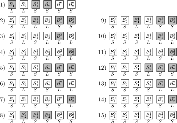
Refer to caption
Figure 3.2: This figure shows an example with three gadgets. It shows the 15 configurations that these gadgets assume during the sequence of 2-changes, excluding the intermediate configurations that arise when one gadget resets another one. Gadgets that are involved in the transformation from configuration ii to configuration i+1i+1 are shown in gray. For example, in the step from the first to the second configuration, the first block ℬ10{\cal B}_{1}^{0} of gadget G0G_{0} resets the two blocks of gadget G1G_{1}. That is, these three blocks follow the sequence of seven 2-changes from Property 5. On the other hand, in the step from the third to the fourth configuration only the first block ℬ12{\cal B}_{1}^{2} of gadget G2G_{2} is involved. It changes from its long state to its short state by a single 2-change. As this figure shows an example with three gadgets, the total number of 2-changes performed according to Lemma 6 is 23+3−0−14=502^{3+3-0}-14=50. This is indeed the case because 6 of the 14 shown steps correspond to sequences of seven 2-changes while 8 steps correspond to single 2-changes.
Lemma 6.

If, for i∈{0,…,n−1}i\in\{0,\ldots,n-1\}, gadget GiG_{i} is in the zero state (L,L)(L,L) and all gadgets GjG_{j} with j>ij>i are in the one state (S,S)(S,S), then there exists a sequence of 2n+3−i−142^{n+3-i}-14 consecutive 2-changes in which only edges of and between the gadgets GjG_{j} with j≥ij\geq i are involved and that terminates in a state in which all gadgets GjG_{j} with j≥ij\geq i are in the one state (S,S)(S,S).

Proof.

We prove the lemma by induction on ii. If gadget Gn−1G_{n-1} is in state (L,L)(L,L), then it can change its state with two 2-changes to (S,S)(S,S) without affecting the other gadgets. This is true because the two blocks of gadget Gn−1G_{n-1} can, one after another, change from their long state Ajn−1​Cjn−1​Bjn−1​Djn−1A^{n-1}_{j}C^{n-1}_{j}B^{n-1}_{j}D^{n-1}_{j} to their short state Ajn−1​Bjn−1​Cjn−1​Djn−1A^{n-1}_{j}B^{n-1}_{j}C^{n-1}_{j}D^{n-1}_{j} by a single 2-change. Hence, the lemma is true for i=n−1i=n-1 because 2n+3−(n−1)−14=22^{n+3-(n-1)}-14=2.

Now assume that the lemma is true for i+1i+1 and consider a state in which gadget GiG_{i} is in state (L,L)(L,L) and all gadgets GjG_{j} with j>ij>i are in state (S,S)(S,S). Due to Property 5, there exists a sequence of seven consecutive 2-changes in which only edges of and between GiG_{i} and Gi+1G_{i+1} are involved, terminating with GiG_{i} being in state (S,L)(S,L) and Gi+1G_{i+1} being in state (L,L)(L,L). By the induction hypothesis there exists a sequence of (2n+2−i−14)(2^{n+2-i}-14) 2-changes after which all gadgets GjG_{j} with j>ij>i are in state (S,S)(S,S). Then, due to Property 5, there exists a sequence of seven consecutive 2-changes in which only GiG_{i} changes its state from (S,L)(S,L) to (S,S)(S,S) while resetting gadget Gi+1G_{i+1} again from (S,S)(S,S) to (L,L)(L,L). Hence, we can apply the induction hypothesis again, yielding that after another (2n+2−i−14)(2^{n+2-i}-14) 2-changes all gadgets GjG_{j} with j≥ij\geq i are in state (S,S)(S,S). This concludes the proof as the number of 2-changes performed is 14+2​(2n+2−i−14)=2n+3−i−1414+2(2^{n+2-i}-14)=2^{n+3-i}-14. ∎

In particular, this implies that, given Property 5, one can construct instances consisting of 2​n2n gadgets, i.e., 16​n16n points, whose state graphs contain paths of length 22​n+3−14>2n+4−222^{2n+3}-14>2^{n+4}-22, as desired in Theorem 1.

3.1.1 Detailed description of the sequence of steps

Now we describe in detail how a sequence of 2-changes satisfying Property 5 can be constructed. First, we assume that gadget GiG_{i} is in state (S,L)(S,L) and that gadget Gi+1G_{i+1} is in state (S,S)(S,S). Under this assumption, there are three consecutive blocks, namely ℬ2i{\cal B}^{i}_{2}, ℬ1i+1{\cal B}^{i+1}_{1}, and ℬ2i+1{\cal B}^{i+1}_{2}, such that the leftmost one ℬ2i{\cal B}^{i}_{2} is in its long state, and the other blocks are in their short states. We need to find a sequence of 2-changes in which only edges of and between these three blocks are involved and after which ℬ2i{\cal B}^{i}_{2} is in its short state and the other blocks are in their long states. Remember that when the edges {u1,u2}\{u_{1},u_{2}\} and {v1,v2}\{v_{1},v_{2}\} are removed from the tour and the vertices appear in the order u1,u2,v1,v2u_{1},u_{2},v_{1},v_{2} in the current tour, then the edges {u1,v1}\{u_{1},v_{1}\} and {u2,v2}\{u_{2},v_{2}\} are added to the tour and the subtour between u1u_{1} and v2v_{2} is visited in reverse order. If, e.g., the current tour corresponds to the permutation (1,2,3,4,5,6,7)(1,2,3,4,5,6,7) and the edges {1,2}\{1,2\} and {5,6}\{5,6\} are removed, then the new tour is (1,5,4,3,2,6,7)(1,5,4,3,2,6,7). The following sequence of 2-changes, which is also shown in Figure 3.3, has the desired properties. Brackets indicate the edges that are removed from the tour.

(a)
Refer to caption
(b)
Refer to caption
(c)
(d)
Refer to caption
(e)
(f)
Refer to caption
(g)
Refer to caption
(h)
Figure 3.3: This figure shows the sequence of seven consecutive 2-changes from Property 5. In each step the thick edges are removed from the tour, and the dotted edges are added to the tour. It shows how block ℬ2i{\cal B}_{2}^{i} switches from its long to its short state while resetting the blocks ℬ1i+1{\cal B}_{1}^{i+1} and ℬ2i+1{\cal B}_{2}^{i+1} from their short to their long states. This figure is only schematic and it does not show the actual geometric embedding of the points into the Euclidean plane.
Long state ACBD Short state ABCD Short state ABCD
1) [A2i\left[A^{i}_{2}\right. C2i]\left.C^{i}_{2}\right] B2iB^{i}_{2} D2iD^{i}_{2} A1i+1A^{i+1}_{1} B1i+1B^{i+1}_{1} C1i+1C^{i+1}_{1} D1i+1D^{i+1}_{1} A2i+1A^{i+1}_{2} B2i+1B^{i+1}_{2} [C2i+1\left[C^{i+1}_{2}\right. D2i+1]\left.D^{i+1}_{2}\right]
2) A2iA^{i}_{2} C2i+1C^{i+1}_{2} [B2i+1\left[B^{i+1}_{2}\right. A2i+1]\left.A^{i+1}_{2}\right] D1i+1D^{i+1}_{1} C1i+1C^{i+1}_{1} B1i+1B^{i+1}_{1} A1i+1A^{i+1}_{1} [D2i\left[D^{i}_{2}\right. B2i]\left.B^{i}_{2}\right] C2iC^{i}_{2} D2i+1D^{i+1}_{2}
3) A2iA^{i}_{2} C2i+1C^{i+1}_{2} [B2i+1\left[B^{i+1}_{2}\right. D2i]\left.D^{i}_{2}\right] A1i+1A^{i+1}_{1} B1i+1B^{i+1}_{1} [C1i+1\left[C^{i+1}_{1}\right. D1i+1]\left.D^{i+1}_{1}\right] A2i+1A^{i+1}_{2} B2iB^{i}_{2} C2iC^{i}_{2} D2i+1D^{i+1}_{2}
4) A2iA^{i}_{2} C2i+1C^{i+1}_{2} B2i+1B^{i+1}_{2} C1i+1C^{i+1}_{1} [B1i+1\left[B^{i+1}_{1}\right. A1i+1]\left.A^{i+1}_{1}\right] D2iD^{i}_{2} D1i+1D^{i+1}_{1} A2i+1A^{i+1}_{2} B2iB^{i}_{2} [C2i\left[C^{i}_{2}\right. D2i+1]\left.D^{i+1}_{2}\right]
5) [A2i\left[A^{i}_{2}\right. C2i+1]\left.C^{i+1}_{2}\right] B2i+1B^{i+1}_{2} C1i+1C^{i+1}_{1} B1i+1B^{i+1}_{1} C2iC^{i}_{2} [B2i\left[B^{i}_{2}\right. A2i+1]\left.A^{i+1}_{2}\right] D1i+1D^{i+1}_{1} D2iD^{i}_{2} A1i+1A^{i+1}_{1} D2i+1D^{i+1}_{2}
6) A2iA^{i}_{2} B2iB^{i}_{2} C2iC^{i}_{2} B1i+1B^{i+1}_{1} [C1i+1\left[C^{i+1}_{1}\right. B2i+1]\left.B^{i+1}_{2}\right] C2i+1C^{i+1}_{2} A2i+1A^{i+1}_{2} D1i+1D^{i+1}_{1} D2iD^{i}_{2} [A1i+1\left[A^{i+1}_{1}\right. D2i+1]\left.D^{i+1}_{2}\right]
7) A2iA^{i}_{2} B2iB^{i}_{2} [C2i\left[C^{i}_{2}\right. B1i+1]\left.B^{i+1}_{1}\right] C1i+1C^{i+1}_{1} A1i+1A^{i+1}_{1} [D2i\left[D^{i}_{2}\right. D1i+1]\left.D^{i+1}_{1}\right] A2i+1A^{i+1}_{2} C2i+1C^{i+1}_{2} B2i+1B^{i+1}_{2} D2i+1D^{i+1}_{2}
A2iA^{i}_{2} B2iB^{i}_{2} C2iC^{i}_{2} D2iD^{i}_{2} A1i+1A^{i+1}_{1} C1i+1C^{i+1}_{1} B1i+1B^{i+1}_{1} D1i+1D^{i+1}_{1} A2i+1A^{i+1}_{2} C2i+1C^{i+1}_{2} B2i+1B^{i+1}_{2} D2i+1D^{i+1}_{2}
Short state ABCD Long state ACBD Long state ACBD

Observe that the configurations 2 to 7 do not have the property mentioned at the beginning of this section that, for every block ℬji{\cal B}^{i}_{j}, the points AjiA^{i}_{j}, BjiB^{i}_{j}, CjiC^{i}_{j}, and DjiD^{i}_{j} are visited consecutively either in the order Aji​Bji​Cji​DjiA^{i}_{j}B^{i}_{j}C^{i}_{j}D^{i}_{j} or in the order Aji​Cji​Bji​DjiA^{i}_{j}C^{i}_{j}B^{i}_{j}D^{i}_{j}. The configurations 2 to 7 are exactly the intermediate configurations that we mentioned at the beginning of this section.

If gadget GiG_{i} is in state (L,L)(L,L) instead of state (S,L)(S,L), a sequence of steps that satisfies Property 5 can be constructed analogously. Additionally, one has to take into account that the three involved blocks ℬ1i{\cal B}^{i}_{1}, ℬ1i+1{\cal B}^{i+1}_{1}, and ℬ2i+1{\cal B}^{i+1}_{2} are not consecutive in the tour but that block ℬ2i{\cal B}^{i}_{2} lies between them. However, one can easily verify that this block is not affected by the sequence of 2-changes, as after the seven 2-changes have been performed, the block is in the same state and at the same position as before.

3.1.2 Embedding the construction into the Euclidean plane

The only missing step in the proof of Theorem 1 for the Euclidean plane is to find points such that all of the 2-changes that we described in the previous section are improving. We specify the positions of the points of gadget Gn−1G_{n-1} and give a rule as to how the points of gadget GiG_{i} can be derived when all points of gadget Gi+1G_{i+1} have already been placed. In our construction it happens that different points have exactly the same coordinates. This is only for ease of notation; if one wants to obtain a TSP instance in which distinct points have distinct coordinates, one can slightly move these points without affecting the property that all 2-changes are improving.

For j∈[2]j\in[2], we choose Ajn−1=(0,0)A^{n-1}_{j}=(0,0), Bjn−1=(1,0)B^{n-1}_{j}=(1,0), Cjn−1=(−0.1,1.4)C^{n-1}_{j}=(-0.1,1.4), and Djn−1=(−1.1,4.8)D^{n-1}_{j}=(-1.1,4.8). Then Ajn−1​Bjn−1​Cjn−1​Djn−1A^{n-1}_{j}B^{n-1}_{j}C^{n-1}_{j}D^{n-1}_{j} is the short state and Ajn−1​Cjn−1​Bjn−1​Djn−1A^{n-1}_{j}C^{n-1}_{j}B^{n-1}_{j}D^{n-1}_{j} is the long state because

𝖽⁡(Ajn−1,Cjn−1)+𝖽⁡(Bjn−1,Djn−1)>𝖽⁡(Ajn−1,Bjn−1)+𝖽⁡(Cjn−1,Djn−1),\dist(A^{n-1}_{j},C^{n-1}_{j})+\dist(B^{n-1}_{j},D^{n-1}_{j})>\dist(A^{n-1}_{j},B^{n-1}_{j})+\dist(C^{n-1}_{j},D^{n-1}_{j}),

as

𝖽⁡(Ajn−1,Cjn−1)+𝖽⁡(Bjn−1,Djn−1)=0.12+1.42+2.12+4.82>6.64\dist(A^{n-1}_{j},C^{n-1}_{j})+\dist(B^{n-1}_{j},D^{n-1}_{j})=\sqrt{0.1^{2}+1.4^{2}}+\sqrt{2.1^{2}+4.8^{2}}>6.64

and

𝖽⁡(Ajn−1,Bjn−1)+𝖽⁡(Cjn−1,Djn−1)=12+02+12+3.42<4.55.\dist(A^{n-1}_{j},B^{n-1}_{j})+\dist(C^{n-1}_{j},D^{n-1}_{j})=\sqrt{1^{2}+0^{2}}+\sqrt{1^{2}+3.4^{2}}<4.55.

We place the points of gadget GiG_{i} as follows (see Figure 3.4):

  1. 1.

    Start with the coordinates of the points of gadget Gi+1G_{i+1}.

  2. 2.

    Rotate these points around the origin by 3​π/23\pi/2.

  3. 3.

    Scale each coordinate by a factor of 3.

  4. 4.

    Translate the points by the vector (−1.2,0.1)(-1.2,0.1).

For j∈[2]j\in[2], this yields Ajn−2=(−1.2,0.1)A^{n-2}_{j}=(-1.2,0.1), Bjn−2=(−1.2,−2.9)B^{n-2}_{j}=(-1.2,-2.9), Cjn−2=(3,0.4)C^{n-2}_{j}=(3,0.4), and Djn−2=(13.2,3.4)D^{n-2}_{j}=(13.2,3.4).

Refer to caption
Figure 3.4: This illustration shows the points of the gadgets Gn−1G_{n-1} and Gn−2G_{n-2}. One can see that Gn−2G_{n-2} is a scaled, rotated, and translated copy of Gn−1G_{n-1}.

From this construction it follows that each gadget is a scaled, rotated, and translated copy of gadget Gn−1G_{n-1}. If one has a set of points in the Euclidean plane that admits certain improving 2-changes, then these 2-changes are still improving if one scales, rotates, and translates all points in the same manner. Hence, it suffices to show that the sequences in which gadget Gn−2G_{n-2} resets gadget Gn−1G_{n-1} from (S,S)(S,S) to (L,L)(L,L) are improving because, for any ii, the points of the gadgets GiG_{i} and Gi+1G_{i+1} are a scaled, rotated, and translated copy of the points of the gadgets Gn−2G_{n-2} and Gn−1G_{n-1}.

There are two sequences in which gadget Gn−2G_{n-2} resets gadget Gn−1G_{n-1} from (S,S)(S,S) to (L,L)(L,L): in the first one, gadget Gn−2G_{n-2} changes its state from (L,L)(L,L) to (S,L)(S,L), in the second one, gadget Gn−2G_{n-2} changes its state from (S,L)(S,L) to (S,S)(S,S). Since the coordinates of the points in both blocks of gadget Gn−2G_{n-2} are the same, the inequalities for both sequences are also identical. The following inequalities show that the improvements made by the steps in both sequences are all positive (see Figure 3.3 or the table in Section 3.1.1 for the sequence of 2-changes):

1)    𝖽⁡(A2n−2,C2n−2)\displaystyle\dist(A^{n-2}_{2},C^{n-2}_{2}) +𝖽⁡(C2n−1,D2n−1)\displaystyle+\dist(C^{n-1}_{2},D^{n-1}_{2}) −𝖽⁡(A2n−2,C2n−1)\displaystyle-\dist(A^{n-2}_{2},C^{n-1}_{2}) −𝖽⁡(C2n−2,D2n−1)\displaystyle-\dist(C^{n-2}_{2},D^{n-1}_{2})\, > 0.03,\displaystyle>\,0.03,
2)    𝖽⁡(B2n−1,A2n−1)\displaystyle\dist(B^{n-1}_{2},A^{n-1}_{2}) +𝖽⁡(D2n−2,B2n−2)\displaystyle+\dist(D^{n-2}_{2},B^{n-2}_{2}) −𝖽⁡(B2n−1,D2n−2)\displaystyle-\dist(B^{n-1}_{2},D^{n-2}_{2}) −𝖽⁡(A2n−1,B2n−2)\displaystyle-\dist(A^{n-1}_{2},B^{n-2}_{2}) > 0.91,\displaystyle>\,0.91,
3)    𝖽⁡(B2n−1,D2n−2)\displaystyle\dist(B^{n-1}_{2},D^{n-2}_{2}) +𝖽⁡(C1n−1,D1n−1)\displaystyle+\dist(C^{n-1}_{1},D^{n-1}_{1}) −𝖽⁡(B2n−1,C1n−1)\displaystyle-\dist(B^{n-1}_{2},C^{n-1}_{1}) −𝖽⁡(D2n−2,D1n−1)\displaystyle-\dist(D^{n-2}_{2},D^{n-1}_{1}) > 0.06,\displaystyle>\,0.06,
4)    𝖽⁡(B1n−1,A1n−1)\displaystyle\dist(B^{n-1}_{1},A^{n-1}_{1}) +𝖽⁡(C2n−2,D2n−1)\displaystyle+\dist(C^{n-2}_{2},D^{n-1}_{2}) −𝖽⁡(B1n−1,C2n−2)\displaystyle-\dist(B^{n-1}_{1},C^{n-2}_{2}) −𝖽⁡(A1n−1,D2n−1)\displaystyle-\dist(A^{n-1}_{1},D^{n-1}_{2}) > 0.05,\displaystyle>\,0.05,
5)    𝖽⁡(A2n−2,C2n−1)\displaystyle\dist(A^{n-2}_{2},C^{n-1}_{2}) +𝖽⁡(B2n−2,A2n−1)\displaystyle+\dist(B^{n-2}_{2},A^{n-1}_{2}) −𝖽⁡(A2n−2,B2n−2)\displaystyle-\dist(A^{n-2}_{2},B^{n-2}_{2}) −𝖽⁡(C2n−1,A2n−1)\displaystyle-\dist(C^{n-1}_{2},A^{n-1}_{2}) > 0.43,\displaystyle>\,0.43,
6)    𝖽⁡(C1n−1,B2n−1)\displaystyle\dist(C^{n-1}_{1},B^{n-1}_{2}) +𝖽⁡(A1n−1,D2n−1)\displaystyle+\dist(A^{n-1}_{1},D^{n-1}_{2}) −𝖽⁡(C1n−1,A1n−1)\displaystyle-\dist(C^{n-1}_{1},A^{n-1}_{1}) −𝖽⁡(B2n−1,D2n−1)\displaystyle-\dist(B^{n-1}_{2},D^{n-1}_{2}) > 0.06,\displaystyle>\,0.06,
7)    𝖽⁡(C2n−2,B1n−1)\displaystyle\dist(C^{n-2}_{2},B^{n-1}_{1}) +𝖽⁡(D2n−2,D1n−1)\displaystyle+\dist(D^{n-2}_{2},D^{n-1}_{1}) −𝖽⁡(C2n−2,D2n−2)\displaystyle-\dist(C^{n-2}_{2},D^{n-2}_{2}) −𝖽⁡(B1n−1,D1n−1)\displaystyle-\dist(B^{n-1}_{1},D^{n-1}_{1}) > 0.53.\displaystyle>\,0.53.

This concludes the proof of Theorem 1 for the Euclidean plane as it shows that all 2-changes in Lemma 6 are improving.

3.2 Exponential Lower Bound for LpL_{p} Metrics

We were not able to find a set of points in the plane such that all 2-changes in Lemma 6 are improving with respect to the Manhattan metric. Therefore, we modify the construction of the gadgets and the sequence of 2-changes. Our construction for the Manhattan metric is based on the construction for the Euclidean plane, but it does not possess the property that every gadget resets its neighboring gadget twice. This property is only true for half of the gadgets. To be more precise, we construct two different types of gadgets which we call reset gadgets and propagation gadgets. Reset gadgets perform the same sequence of 2-changes as the gadgets that we constructed for the Euclidean plane. Propagation gadgets also have the same structure as the gadgets for the Euclidean plane, but when such a gadget changes its state from (L,L)(L,L) to (S,S)(S,S), it resets its neighboring gadget only once. Due to this relaxed requirement it is possible to find points in the Manhattan plane whose distances satisfy all necessary inequalities. Instead of nn gadgets, our construction consists of 2​n2n gadgets, namely nn propagation gadgets G0P,…,Gn−1PG_{0}^{P},\ldots,G_{n-1}^{P} and nn reset gadgets G0R,…,Gn−1RG_{0}^{R},\ldots,G_{n-1}^{R}. The order in which these gadgets appear in the tour is G0P​G0R​G1P​G1R​…​Gn−1P​Gn−1RG_{0}^{P}G_{0}^{R}G_{1}^{P}G_{1}^{R}\ldots G_{n-1}^{P}G_{n-1}^{R}.

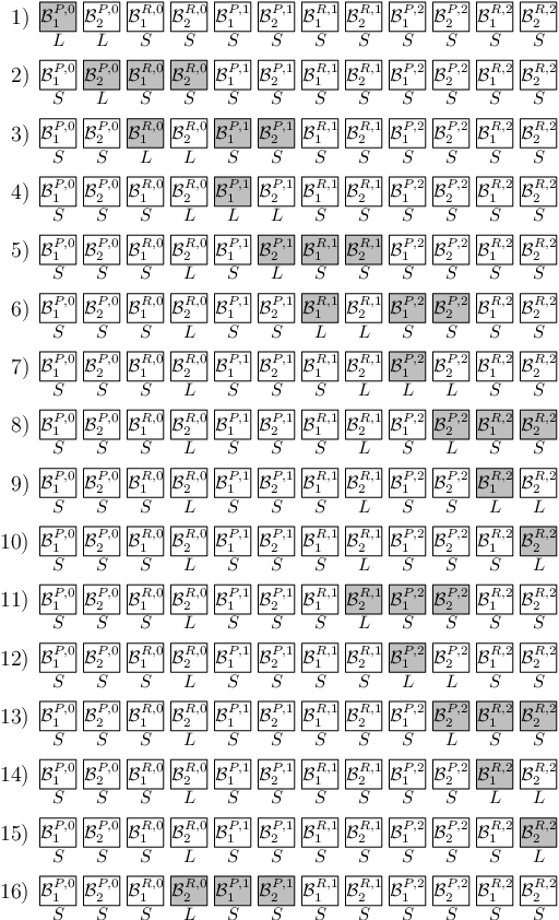
As before, every gadget consists of two blocks and the order in which the blocks and the gadgets are visited does not change during the sequence of 2-changes. Consider a reset gadget GiRG^{R}_{i} and its neighboring propagation gadget Gi+1PG^{P}_{i+1}. We will embed the points of the gadgets into the Manhattan plane in such a way that Property 5 is still satisfied. That is, if GiRG^{R}_{i} is in state (L,L)(L,L) (or state (S,L)(S,L), respectively) and Gi+1PG^{P}_{i+1} is in state (S,S)(S,S), then there exists a sequence of seven consecutive 2-changes resetting gadget Gi+1PG^{P}_{i+1} to state (L,L)(L,L) and leaving gadget GiRG^{R}_{i} in state (S,L)(S,L) (or (S,S)(S,S), respectively). The situation is different for a propagation gadget GiPG^{P}_{i} and its neighboring reset gadget GiRG^{R}_{i}. In this case, if GiPG^{P}_{i} is in state (L,L)(L,L), it first changes its state with a single 2-change to (S,L)(S,L). After that, gadget GiPG^{P}_{i} changes its state to (S,S)(S,S) while resetting gadget GiRG^{R}_{i} from state (S,S)(S,S) to state (L,L)(L,L) by a sequence of seven consecutive 2-changes. In both cases, the sequences of 2-changes in which one block changes from its long to its short state while resetting two blocks of the neighboring gadget from their short to their long states are chosen analogously to the ones for the Euclidean plane described in Section 3.1.1. An example with three propagation and three reset gadgets is shown in Figure 3.5.

In the initial tour, only gadget G0PG^{P}_{0} is in state (L,L)(L,L) and every other gadget is in state (S,S)(S,S). With similar arguments as for the Euclidean plane, we can show that gadget GiRG_{i}^{R} is reset from its one state (S,S)(S,S) to its zero state (L,L)(L,L) 2i2^{i} times and that the total number of steps is 2n+4−222^{n+4}-22.

Refer to caption
Figure 3.5: This figure shows an example with three propagation and three reset gadgets. It shows the first 16 configurations that these gadgets assume during the sequence of 2-changes, excluding the intermediate configurations that arise when one gadget resets another one. Gadgets that are involved in the transformation from configuration ii to configuration i+1i+1 are shown in gray. For example, in the step from the first to the second configuration, the first block ℬ1P,0{\cal B}_{1}^{P,0} of the first propagation gadget G0PG_{0}^{P} switches from its long to its short state by a single 2-change. Then in the step from the second to the third configuration, the second block ℬ2P,0{\cal B}_{2}^{P,0} of the first propagation gadget G0PG_{0}^{P} resets the two blocks of the first reset gadget G0RG_{0}^{R}. That is, these three blocks follow the sequence of seven 2-changes from Property 5.

3.2.1 Embedding the construction into the Manhattan plane

As in the construction in the Euclidean plane, the points in both blocks of a reset gadget GiRG_{i}^{R} have the same coordinates. Also in this case one can slightly move all the points without affecting the inequalities if one wants distinct coordinates for distinct points. Again, we choose points for the gadgets Gn−1PG_{n-1}^{P} and Gn−1RG_{n-1}^{R} and describe how the points of the gadgets GiPG_{i}^{P} and GiRG_{i}^{R} can be chosen when the points of the gadgets Gi+1PG_{i+1}^{P} and Gi+1RG_{i+1}^{R} are already chosen. For j∈[2]j\in[2], we choose AR,jn−1=(0,1)A^{n-1}_{R,j}=(0,1), BR,jn−1=(0,0)B^{n-1}_{R,j}=(0,0), CR,jn−1=(−0.7,0.1)C^{n-1}_{R,j}=(-0.7,0.1), and DR,jn−1=(−1.2,0.08)D^{n-1}_{R,j}=(-1.2,0.08). Furthermore, we choose AP,1n−1=(−2,1.8)A^{n-1}_{P,1}=(-2,1.8), BP,1n−1=(−3.3,2.8)B^{n-1}_{P,1}=(-3.3,2.8), CP,1n−1=(−1.3,1.4)C^{n-1}_{P,1}=(-1.3,1.4), DP,1n−1=(1.5,0.9)D^{n-1}_{P,1}=(1.5,0.9), AP,2n−1=(−0.7,1.6)A^{n-1}_{P,2}=(-0.7,1.6), BP,2n−1=(−1.5,1.2)B^{n-1}_{P,2}=(-1.5,1.2), CP,2n−1=(1.9,−1.5)C^{n-1}_{P,2}=(1.9,-1.5), and DP,2n−1=(−0.8,−1.1)D^{n-1}_{P,2}=(-0.8,-1.1).

Before we describe how the points of the other gadgets are chosen, we first show that the 2-changes within and between the gadgets Gn−1PG_{n-1}^{P} and Gn−1RG_{n-1}^{R} are improving. For j∈[2]j\in[2], AR,jn−1​BR,jn−1​CR,jn−1​DR,jn−1A^{n-1}_{R,j}B^{n-1}_{R,j}C^{n-1}_{R,j}D^{n-1}_{R,j} is the short state because

𝖽⁡(AR,jn−1,CR,jn−1)+𝖽⁡(BR,jn−1,DR,jn−1)−(𝖽⁡(AR,jn−1,BR,jn−1)+𝖽⁡(CR,jn−1,DR,jn−1))\displaystyle\quad\dist(A^{n-1}_{R,j},C^{n-1}_{R,j})+\dist(B^{n-1}_{R,j},D^{n-1}_{R,j})-(\dist(A^{n-1}_{R,j},B^{n-1}_{R,j})+\dist(C^{n-1}_{R,j},D^{n-1}_{R,j}))
=(0.7+0.9)+(1.2+0.08)−(0+1)−(0.5+0.02)=1.36.\displaystyle=(0.7+0.9)+(1.2+0.08)-(0+1)-(0.5+0.02)=1.36.

In the 2-change in which Gn−1PG_{n-1}^{P} changes its state from (L,L)(L,L) to (S,L)(S,L) the edges AP,1n−1,CP,1n−1A^{n-1}_{P,1},C^{n-1}_{P,1} and BP,1n−1,DP,1n−1B^{n-1}_{P,1},D^{n-1}_{P,1} are replaced with the edges AP,1n−1,BP,1n−1A^{n-1}_{P,1},B^{n-1}_{P,1} and CP,1n−1,DP,1n−1C^{n-1}_{P,1},D^{n-1}_{P,1}. This 2-change is improving because

𝖽⁡(AP,1n−1,CP,1n−1)+𝖽⁡(BP,1n−1,DP,1n−1)−(𝖽⁡(AP,1n−1,BP,1n−1)+𝖽⁡(CP,1n−1,DP,1n−1))\displaystyle\quad\dist(A^{n-1}_{P,1},C^{n-1}_{P,1})+\dist(B^{n-1}_{P,1},D^{n-1}_{P,1})-(\dist(A^{n-1}_{P,1},B^{n-1}_{P,1})+\dist(C^{n-1}_{P,1},D^{n-1}_{P,1}))
=(0.7+0.4)+(4.8+1.9)−(1.3+1)−(2.8+0.5)=2.2.\displaystyle=(0.7+0.4)+(4.8+1.9)-(1.3+1)-(2.8+0.5)=2.2.

The 2-changes in the sequence in which Gn−1PG_{n-1}^{P} changes its state from (S,L)(S,L) to (S,S)(S,S) while resetting Gn−1RG_{n-1}^{R} are chosen analogously to the ones shown in Figure 3.3 and in the table in Section 3.1.1. The only difference is that the involved blocks are not ℬ2i{\cal B}^{i}_{2}, ℬ1i+1{\cal B}^{i+1}_{1}, and ℬ2i+1{\cal B}^{i+1}_{2} anymore, but the second block of gadget Gn−1PG_{n-1}^{P} and the two blocks of gadget Gn−1RG_{n-1}^{R}, respectively. This gives rise to the following equalities that show that the improvements made by the 2-changes in this sequence are all positive:

1)    𝖽⁡(AP,2n−1,CP,2n−1)\displaystyle\dist(A^{n-1}_{P,2},C^{n-1}_{P,2}) +𝖽⁡(CR,2n−1,DR,2n−1)\displaystyle+\dist(C^{n-1}_{R,2},D^{n-1}_{R,2}) −𝖽⁡(AP,2n−1,CR,2n−1)\displaystyle-\dist(A^{n-1}_{P,2},C^{n-1}_{R,2}) −𝖽⁡(CP,2n−1,DR,2n−1)\displaystyle-\dist(C^{n-1}_{P,2},D^{n-1}_{R,2})\, = 0.04,\displaystyle=\,0.04,
2)    𝖽⁡(BR,2n−1,AR,2n−1)\displaystyle\dist(B^{n-1}_{R,2},A^{n-1}_{R,2}) +𝖽⁡(DP,2n−1,BP,2n−1)\displaystyle+\dist(D^{n-1}_{P,2},B^{n-1}_{P,2}) −𝖽⁡(BR,2n−1,DP,2n−1)\displaystyle-\dist(B^{n-1}_{R,2},D^{n-1}_{P,2}) −𝖽⁡(AR,2n−1,BP,2n−1)\displaystyle-\dist(A^{n-1}_{R,2},B^{n-1}_{P,2}) = 0.4,\displaystyle=\,0.4,
3)    𝖽⁡(BR,2n−1,DP,2n−1)\displaystyle\dist(B^{n-1}_{R,2},D^{n-1}_{P,2}) +𝖽⁡(CR,1n−1,DR,1n−1)\displaystyle+\dist(C^{n-1}_{R,1},D^{n-1}_{R,1}) −𝖽⁡(BR,2n−1,CR,1n−1)\displaystyle-\dist(B^{n-1}_{R,2},C^{n-1}_{R,1}) −𝖽⁡(DP,2n−1,DR,1n−1)\displaystyle-\dist(D^{n-1}_{P,2},D^{n-1}_{R,1}) = 0.04,\displaystyle=\,0.04,
4)    𝖽⁡(BR,1n−1,AR,1n−1)\displaystyle\dist(B^{n-1}_{R,1},A^{n-1}_{R,1}) +𝖽⁡(CP,2n−1,DR,2n−1)\displaystyle+\dist(C^{n-1}_{P,2},D^{n-1}_{R,2}) −𝖽⁡(BR,1n−1,CP,2n−1)\displaystyle-\dist(B^{n-1}_{R,1},C^{n-1}_{P,2}) −𝖽⁡(AR,1n−1,DR,2n−1)\displaystyle-\dist(A^{n-1}_{R,1},D^{n-1}_{R,2}) = 0.16,\displaystyle=\,0.16,
5)    𝖽⁡(AP,2n−1,CR,2n−1)\displaystyle\dist(A^{n-1}_{P,2},C^{n-1}_{R,2}) +𝖽⁡(BP,2n−1,AR,2n−1)\displaystyle+\dist(B^{n-1}_{P,2},A^{n-1}_{R,2}) −𝖽⁡(AP,2n−1,BP,2n−1)\displaystyle-\dist(A^{n-1}_{P,2},B^{n-1}_{P,2}) −𝖽⁡(CR,2n−1,AR,2n−1)\displaystyle-\dist(C^{n-1}_{R,2},A^{n-1}_{R,2}) = 0.4,\displaystyle=\,0.4,
6)    𝖽⁡(CR,1n−1,BR,2n−1)\displaystyle\dist(C^{n-1}_{R,1},B^{n-1}_{R,2}) +𝖽⁡(AR,1n−1,DR,2n−1)\displaystyle+\dist(A^{n-1}_{R,1},D^{n-1}_{R,2}) −𝖽⁡(CR,1n−1,AR,1n−1)\displaystyle-\dist(C^{n-1}_{R,1},A^{n-1}_{R,1}) −𝖽⁡(BR,2n−1,DR,2n−1)\displaystyle-\dist(B^{n-1}_{R,2},D^{n-1}_{R,2}) = 0.04,\displaystyle=\,0.04,
7)    𝖽⁡(CP,2n−1,BR,1n−1)\displaystyle\dist(C^{n-1}_{P,2},B^{n-1}_{R,1}) +𝖽⁡(DP,2n−1,DR,1n−1)\displaystyle+\dist(D^{n-1}_{P,2},D^{n-1}_{R,1}) −𝖽⁡(CP,2n−1,DP,2n−1)\displaystyle-\dist(C^{n-1}_{P,2},D^{n-1}_{P,2}) −𝖽⁡(BR,1n−1,DR,1n−1)\displaystyle-\dist(B^{n-1}_{R,1},D^{n-1}_{R,1}) = 0.6.\displaystyle=\,0.6.

Again, our construction possesses the property that each pair of gadgets GiPG_{i}^{P} and GiRG_{i}^{R} is a scaled and translated version of the pair Gn−1PG_{n-1}^{P} and Gn−1RG_{n-1}^{R}. Since we have relaxed the requirements for the gadgets, we do not even need rotations here. We place the points of GiPG_{i}^{P} and GiRG_{i}^{R} as follows:

  1. 1.

    Start with the coordinates specified for the points of gadgets Gi+1PG_{i+1}^{P} and Gi+1RG_{i+1}^{R}.

  2. 2.

    Scale each coordinate by a factor of 7.7.

  3. 3.

    Translate the points by the vector (1.93,0.3)(1.93,0.3).

For j∈[2]j\in[2], this yields AR,jn−2=(1.93,8)A^{n-2}_{R,j}=(1.93,8), BR,jn−2=(1.93,0.3)B^{n-2}_{R,j}=(1.93,0.3), CR,jn−2=(−3.46,1.07)C^{n-2}_{R,j}=(-3.46,1.07), and DR,jn−2=(−7.31,0.916)D^{n-2}_{R,j}=(-7.31,0.916). Additionally, it yields AP,1n−2=(−13.47,14.16)A^{n-2}_{P,1}=(-13.47,14.16), BP,1n−2=(−23.48,21.86)B^{n-2}_{P,1}=(-23.48,21.86), CP,1n−2=(−8.08,11.08)C^{n-2}_{P,1}=(-8.08,11.08), DP,1n−2=(13.48,7.23)D^{n-2}_{P,1}=(13.48,7.23), AP,2n−2=(−3.46,12.62)A^{n-2}_{P,2}=(-3.46,12.62), BP,2n−2=(−9.62,9.54)B^{n-2}_{P,2}=(-9.62,9.54), CP,2n−2=(16.56,−11.25)C^{n-2}_{P,2}=(16.56,-11.25), and DP,2n−2=(−4.23,−8.17)D^{n-2}_{P,2}=(-4.23,-8.17).

As in our construction for the Euclidean plane, it suffices to show that the sequences in which gadget Gn−2RG^{R}_{n-2} resets gadget Gn−1PG^{P}_{n-1} from (S,S)(S,S) to (L,L)(L,L) are improving because, for any ii, the points of the gadgets GiRG^{R}_{i} and Gi+1PG^{P}_{i+1} are a scaled and translated copy of the points of the gadgets Gn−2RG^{R}_{n-2} and Gn−1PG^{P}_{n-1}. The 2-changes in these sequences are chosen analogously to the ones shown in Figure 3.3 and in the table in Section 3.1.1. The only difference is that the involved blocks are not ℬ2i{\cal B}^{i}_{2}, ℬ1i+1{\cal B}^{i+1}_{1}, and ℬ2i+1{\cal B}^{i+1}_{2} anymore, but one of the blocks of gadget Gn−2RG^{R}_{n-2} and the two blocks of gadget Gn−1PG^{P}_{n-1}, respectively. As the coordinates of the points in the two blocks of gadget Gn−2RG^{R}_{n-2} are the same, the inequalities for both sequences are also identical. The improvements made by the steps in both sequences are

1)    𝖽⁡(AR,2n−2,CR,2n−2)\displaystyle\dist(A^{n-2}_{R,2},C^{n-2}_{R,2}) +𝖽⁡(CP,2n−1,DP,2n−1)\displaystyle+\dist(C^{n-1}_{P,2},D^{n-1}_{P,2}) −𝖽⁡(AR,2n−2,CP,2n−1)\displaystyle-\dist(A^{n-2}_{R,2},C^{n-1}_{P,2}) −𝖽⁡(CR,2n−2,DP,2n−1)\displaystyle-\dist(C^{n-2}_{R,2},D^{n-1}_{P,2})\, = 1.06\displaystyle=\,1.06
2)    𝖽⁡(BP,2n−1,AP,2n−1)\displaystyle\dist(B^{n-1}_{P,2},A^{n-1}_{P,2}) +𝖽⁡(DR,2n−2,BR,2n−2)\displaystyle+\dist(D^{n-2}_{R,2},B^{n-2}_{R,2}) −𝖽⁡(BP,2n−1,DR,2n−2)\displaystyle-\dist(B^{n-1}_{P,2},D^{n-2}_{R,2}) −𝖽⁡(AP,2n−1,BR,2n−2)\displaystyle-\dist(A^{n-1}_{P,2},B^{n-2}_{R,2})\, = 1.032,\displaystyle=\,1.032,
3)    𝖽⁡(BP,2n−1,DR,2n−2)\displaystyle\dist(B^{n-1}_{P,2},D^{n-2}_{R,2}) +𝖽⁡(CP,1n−1,DP,1n−1)\displaystyle+\dist(C^{n-1}_{P,1},D^{n-1}_{P,1}) −𝖽⁡(BP,2n−1,CP,1n−1)\displaystyle-\dist(B^{n-1}_{P,2},C^{n-1}_{P,1}) −𝖽⁡(DR,2n−2,DP,1n−1)\displaystyle-\dist(D^{n-2}_{R,2},D^{n-1}_{P,1})\, = 0.168,\displaystyle=\,0.168,
4)    𝖽⁡(BP,1n−1,AP,1n−1)\displaystyle\dist(B^{n-1}_{P,1},A^{n-1}_{P,1}) +𝖽⁡(CR,2n−2,DP,2n−1)\displaystyle+\dist(C^{n-2}_{R,2},D^{n-1}_{P,2}) −𝖽⁡(BP,1n−1,CR,2n−2)\displaystyle-\dist(B^{n-1}_{P,1},C^{n-2}_{R,2}) −𝖽⁡(AP,1n−1,DP,2n−1)\displaystyle-\dist(A^{n-1}_{P,1},D^{n-1}_{P,2})\, = 1.14,\displaystyle=\,1.14,
5)    𝖽⁡(AR,2n−2,CP,2n−1)\displaystyle\dist(A^{n-2}_{R,2},C^{n-1}_{P,2}) +𝖽⁡(BR,2n−2,AP,2n−1)\displaystyle+\dist(B^{n-2}_{R,2},A^{n-1}_{P,2}) −𝖽⁡(AR,2n−2,BR,2n−2)\displaystyle-\dist(A^{n-2}_{R,2},B^{n-2}_{R,2}) −𝖽⁡(CP,2n−1,AP,2n−1)\displaystyle-\dist(C^{n-1}_{P,2},A^{n-1}_{P,2})\, = 0.06,\displaystyle=\,0.06,
6)    𝖽⁡(CP,1n−1,BP,2n−1)\displaystyle\dist(C^{n-1}_{P,1},B^{n-1}_{P,2}) +𝖽⁡(AP,1n−1,DP,2n−1)\displaystyle+\dist(A^{n-1}_{P,1},D^{n-1}_{P,2}) −𝖽⁡(CP,1n−1,AP,1n−1)\displaystyle-\dist(C^{n-1}_{P,1},A^{n-1}_{P,1}) −𝖽⁡(BP,2n−1,DP,2n−1)\displaystyle-\dist(B^{n-1}_{P,2},D^{n-1}_{P,2})\, = 0.4,\displaystyle=\,0.4,
7)    𝖽⁡(CR,2n−2,BP,1n−1)\displaystyle\dist(C^{n-2}_{R,2},B^{n-1}_{P,1}) +𝖽⁡(DR,2n−2,DP,1n−1)\displaystyle+\dist(D^{n-2}_{R,2},D^{n-1}_{P,1}) −𝖽⁡(CR,2n−2,DR,2n−2)\displaystyle-\dist(C^{n-2}_{R,2},D^{n-2}_{R,2}) −𝖽⁡(BP,1n−1,DP,1n−1)\displaystyle-\dist(B^{n-1}_{P,1},D^{n-1}_{P,1})\, = 0.012.\displaystyle=\,0.012.

This concludes the proof of Theorem 1 for the Manhattan metric as it shows that all 2-changes are improving.

Let us remark that this also implies Theorem 1 for the L∞L_{\infty} metric because distances with respect to the L∞L_{\infty} metric coincide with distances with respect to the Manhattan metric if one rotates all points by π/4\pi/4 around the origin and scales every coordinate by 1/21/\sqrt{2}.

3.2.2 Embedding the construction into general LpL_{p} metrics

It is also possible to embed our Manhattan construction into the LpL_{p} metric for p∈ℕp\in\mathbb{N} with p≥3p\geq 3. For j∈[2]j\in[2], we choose AR,jn−1=(0,1)A^{n-1}_{R,j}=(0,1), BR,jn−1=(0,0)B^{n-1}_{R,j}=(0,0), CR,jn−1=(3.5,3.7)C^{n-1}_{R,j}=(3.5,3.7), and DR,jn−1=(7.8,−3.2)D^{n-1}_{R,j}=(7.8,-3.2). Moreover, we choose AP,1n−1=(−2.5,−2.4)A^{n-1}_{P,1}=(-2.5,-2.4), BP,1n−1=(−4.7,−7.3)B^{n-1}_{P,1}=(-4.7,-7.3), CP,1n−1=(−8.6,−4.6)C^{n-1}_{P,1}=(-8.6,-4.6), DP,1n−1=(3.7,9.8)D^{n-1}_{P,1}=(3.7,9.8), AP,2n−1=(3.2,2)A^{n-1}_{P,2}=(3.2,2), BP,2n−1=(7.2,7.2)B^{n-1}_{P,2}=(7.2,7.2), CP,2n−1=(−6.5,−1.6)C^{n-1}_{P,2}=(-6.5,-1.6), and DP,2n−1=(−1.5,−7.1)D^{n-1}_{P,2}=(-1.5,-7.1). We place the points of GiPG_{i}^{P} and GiRG_{i}^{R} as follows:

  1. 1.

    Start with the coordinates specified for the points of gadgets Gi+1PG_{i+1}^{P} and Gi+1RG_{i+1}^{R}.

  2. 2.

    Rotate these points around the origin by π\pi.

  3. 3.

    Scale each coordinate by a factor of 7.8.

  4. 4.

    Translate the points by the vector (7.2,5.3)(7.2,5.3).

For j∈[2]j\in[2], this yields AR,jn−2=(7.2,−2.5)A^{n-2}_{R,j}=(7.2,-2.5), BR,jn−2=(7.2,5.3)B^{n-2}_{R,j}=(7.2,5.3), CR,jn−2=(−20.1,−23.56)C^{n-2}_{R,j}=(-20.1,-23.56), and DR,jn−2=(−53.64,30.26)D^{n-2}_{R,j}=(-53.64,30.26). Additionally, it yields AP,1n−2=(26.7,24.02)A^{n-2}_{P,1}=(26.7,24.02), BP,1n−2=(43.86,62.24)B^{n-2}_{P,1}=(43.86,62.24), CP,1n−2=(74.28,41.18)C^{n-2}_{P,1}=(74.28,41.18), DP,1n−2=(−21.66,−71.14)D^{n-2}_{P,1}=(-21.66,-71.14), AP,2n−2=(−17.76,−10.3)A^{n-2}_{P,2}=(-17.76,-10.3), BP,2n−2=(−48.96,−50.86)B^{n-2}_{P,2}=(-48.96,-50.86), CP,2n−2=(57.9,17.78)C^{n-2}_{P,2}=(57.9,17.78), and DP,2n−2=(18.9,60.68)D^{n-2}_{P,2}=(18.9,60.68).

It needs to be shown that the distances of these points when measured according to the LpL_{p} metric for any p∈ℕp\in\mathbb{N} with p≥3p\geq 3 satisfy all necessary inequalities, that is, all 16 inequalities that we have verified in the previous section for the Manhattan metric. Let us start by showing that for j∈[2]j\in[2], AR,jn−1​BR,jn−1​CR,jn−1​DR,jn−1A^{n-1}_{R,j}B^{n-1}_{R,j}C^{n-1}_{R,j}D^{n-1}_{R,j} is the short state. For this, we have to prove the following inequality for every p∈ℕp\in\mathbb{N} with p≥3p\geq 3:

𝖽p⁡(AR,jn−1,CR,jn−1)+𝖽p⁡(BR,jn−1,DR,jn−1)−(𝖽p⁡(AR,jn−1,BR,jn−1)+𝖽p⁡(CR,jn−1,DR,jn−1))>0\displaystyle\dist_{p}(A^{n-1}_{R,j},C^{n-1}_{R,j})\!+\!\dist_{p}(B^{n-1}_{R,j},D^{n-1}_{R,j})\!-\!(\dist_{p}(A^{n-1}_{R,j},B^{n-1}_{R,j})\!+\!\dist_{p}(C^{n-1}_{R,j},D^{n-1}_{R,j}))>0
⇔3.5p+2.7pp+7.8p+3.2pp−0p+1pp−4.3p+6.9pp>0.\displaystyle\iff\,\,\,\sqrt[p]{3.5^{p}+2.7^{p}}+\sqrt[p]{7.8^{p}+3.2^{p}}-\sqrt[p]{0^{p}+1^{p}}-\sqrt[p]{4.3^{p}+6.9^{p}}\,>0. (3.1)

For p=∞p=\infty, the inequality is satisfied as the left side equals 3.43.4 when distances are measured according to the L∞L_{\infty} metric. In order to show that the inequality is also satisfied for every p∈ℕp\in\mathbb{N} with p≥3p\geq 3, we analyze by how much the distances 𝖽p\dist_{p} deviate from the distances 𝖽∞\dist_{\infty}. For p∈ℕp\in\mathbb{N} with p≥3p\geq 3, we obtain

4.3p+6.9pp−6.9=6.9⋅(1+(4.36.9)pp−1)≤ 6.9⋅(1+(4.36.9)33−1)<0.52.\textstyle\begin{split}&\sqrt[p]{4.3^{p}+6.9^{p}}-6.9=6.9\cdot\left(\sqrt[p]{1+\left(\frac{4.3}{6.9}\right)^{p}}-1\right)\\ \leq&\,6.9\cdot\left(\sqrt[3]{1+\left(\frac{4.3}{6.9}\right)^{3}}-1\right)<0.52.\end{split} (3.2)

Hence,

3.5p+2.7pp+7.8p+3.2pp−0p+1pp−4.3p+6.9pp\displaystyle\sqrt[p]{3.5^{p}+2.7^{p}}+\sqrt[p]{7.8^{p}+3.2^{p}}-\sqrt[p]{0^{p}+1^{p}}-\sqrt[p]{4.3^{p}+6.9^{p}}
≥\displaystyle\geq  3.5+7.8−1−6.9−0.52>0,\displaystyle\,3.5+7.8-1-6.9-0.52>0,

which proves that AR,jn−1​BR,jn−1​CR,jn−1​DR,jn−1A^{n-1}_{R,j}B^{n-1}_{R,j}C^{n-1}_{R,j}D^{n-1}_{R,j} is the short state for every p∈ℕp\in\mathbb{N} with p≥3p\geq 3.

Next we argue that also the 2-change in which Gn−1PG_{n-1}^{P} changes its state from (L,L)(L,L) to (S,L)(S,L) is improving. For this, the following inequality needs to be verified for every p∈ℕp\in\mathbb{N} with p≥3p\geq 3:

𝖽⁡(AP,1n−1,CP,1n−1)+𝖽⁡(BP,1n−1,DP,1n−1)−(𝖽⁡(AP,1n−1,BP,1n−1)−𝖽⁡(CP,1n−1,DP,1n−1))>0\displaystyle\dist(A^{n-1}_{P,1},C^{n-1}_{P,1})+\dist(B^{n-1}_{P,1},D^{n-1}_{P,1})-(\dist(A^{n-1}_{P,1},B^{n-1}_{P,1})-\dist(C^{n-1}_{P,1},D^{n-1}_{P,1}))>0
⇔6.1p+2.2pp+8.4p+17.1pp−2.2p+4.9pp−12.3p+14.4pp>0.\displaystyle\iff\,\,\,\sqrt[p]{6.1^{p}+2.2^{p}}+\sqrt[p]{8.4^{p}+17.1^{p}}-\sqrt[p]{2.2^{p}+4.9^{p}}-\sqrt[p]{12.3^{p}+14.4^{p}}>0.

As before, we obtain for p∈ℕp\in\mathbb{N} with p≥3p\geq 3

2.2p+4.9pp−4.9=4.9⋅(1+(2.24.9)pp−1)≤4.9⋅(1+(2.24.9)33−1)<0.15\textstyle\sqrt[p]{2.2^{p}+4.9^{p}}-4.9=4.9\cdot\left(\sqrt[p]{1+\left(\frac{2.2}{4.9}\right)^{p}}\!-\!1\right)\leq 4.9\cdot\left(\sqrt[3]{1+\left(\frac{2.2}{4.9}\right)^{3}}\!-\!1\right)<0.15

and

12.3p+14.4pp−14.4=14.4⋅(1+(12.314.4)pp−1)\displaystyle\sqrt[p]{12.3^{p}+14.4^{p}}-14.4=14.4\cdot\left(\sqrt[p]{1+\left(\frac{12.3}{14.4}\right)^{p}}-1\right)
≤\displaystyle\leq  14.4⋅(1+(12.314.4)33−1)<2.53.\displaystyle\,14.4\cdot\left(\sqrt[3]{1+\left(\frac{12.3}{14.4}\right)^{3}}-1\right)<2.53.

This implies for p∈ℕp\in\mathbb{N} with p≥3p\geq 3

6.1p+2.2pp+8.4p+17.1pp−2.2p+4.9pp−12.3p+14.4pp\displaystyle\quad\sqrt[p]{6.1^{p}+2.2^{p}}+\sqrt[p]{8.4^{p}+17.1^{p}}-\sqrt[p]{2.2^{p}+4.9^{p}}-\sqrt[p]{12.3^{p}+14.4^{p}}
≥6.1+17.1−4.9−0.15−14.4−2.53>0,\displaystyle\geq 6.1+17.1-4.9-0.15-14.4-2.53>0,

which proves that the 2-change in which Gn−1PG_{n-1}^{P} changes its state from (L,L)(L,L) to (S,L)(S,L) is improving for every p∈ℕp\in\mathbb{N} with p≥3p\geq 3.

Next we show that the improvements made by the 2-changes in the sequence in which Gn−1PG_{n-1}^{P} changes its state from (S,L)(S,L) to (S,S)(S,S) while resetting Gn−1RG_{n-1}^{R} are positive. For this we need to verify the following inequalities for every p∈ℕp\in\mathbb{N} with p≥3p\geq 3 (observe that these are exactly the same inequalities that we have verified in Section 3.2.1 for the Manhattan metric):

1)    𝖽p⁡(AP,2n−1,CP,2n−1)\displaystyle\dist_{p}(A^{n-1}_{P,2},C^{n-1}_{P,2}) +𝖽p⁡(CR,2n−1,DR,2n−1)\displaystyle+\dist_{p}(C^{n-1}_{R,2},D^{n-1}_{R,2}) −𝖽p⁡(AP,2n−1,CR,2n−1)\displaystyle-\dist_{p}(A^{n-1}_{P,2},C^{n-1}_{R,2}) −𝖽p⁡(CP,2n−1,DR,2n−1)\displaystyle-\dist_{p}(C^{n-1}_{P,2},D^{n-1}_{R,2})\, > 0\displaystyle>\,0
⇔\displaystyle\iff\,\,\, 9.7p+3.6pp\displaystyle\sqrt[p]{9.7^{p}+3.6^{p}} +4.3p+6.9pp\displaystyle+\sqrt[p]{4.3^{p}+6.9^{p}} −0.3p+1.7pp\displaystyle-\sqrt[p]{0.3^{p}+1.7^{p}} −14.3p+1.6pp\displaystyle-\sqrt[p]{14.3^{p}+1.6^{p}} >0,\displaystyle\,>0,
2)    𝖽p⁡(BR,2n−1,AR,2n−1)\displaystyle\dist_{p}(B^{n-1}_{R,2},A^{n-1}_{R,2}) +𝖽p⁡(DP,2n−1,BP,2n−1)\displaystyle+\dist_{p}(D^{n-1}_{P,2},B^{n-1}_{P,2}) −𝖽p⁡(BR,2n−1,DP,2n−1)\displaystyle-\dist_{p}(B^{n-1}_{R,2},D^{n-1}_{P,2}) −𝖽p⁡(AR,2n−1,BP,2n−1)\displaystyle-\dist_{p}(A^{n-1}_{R,2},B^{n-1}_{P,2}) > 0\displaystyle>\,0
⇔\displaystyle\iff\,\,\, 0.0p+1.0pp\displaystyle\sqrt[p]{0.0^{p}+1.0^{p}} +8.7p+14.3pp\displaystyle+\sqrt[p]{8.7^{p}+14.3^{p}} −1.5p+7.1pp\displaystyle-\sqrt[p]{1.5^{p}+7.1^{p}} −7.2p+6.2pp\displaystyle-\sqrt[p]{7.2^{p}+6.2^{p}} >0,\displaystyle\,>0,
3)    𝖽p⁡(BR,2n−1,DP,2n−1)\displaystyle\dist_{p}(B^{n-1}_{R,2},D^{n-1}_{P,2}) +𝖽p⁡(CR,1n−1,DR,1n−1)\displaystyle+\dist_{p}(C^{n-1}_{R,1},D^{n-1}_{R,1}) −𝖽p⁡(BR,2n−1,CR,1n−1)\displaystyle-\dist_{p}(B^{n-1}_{R,2},C^{n-1}_{R,1}) −𝖽p⁡(DP,2n−1,DR,1n−1)\displaystyle-\dist_{p}(D^{n-1}_{P,2},D^{n-1}_{R,1}) > 0\displaystyle>\,0
⇔\displaystyle\iff\,\,\, 1.5p+7.1pp\displaystyle\sqrt[p]{1.5^{p}+7.1^{p}} +4.3p+6.9pp\displaystyle+\sqrt[p]{4.3^{p}+6.9^{p}} −3.5p+3.7pp\displaystyle-\sqrt[p]{3.5^{p}+3.7^{p}} −9.3p+3.9pp\displaystyle-\sqrt[p]{9.3^{p}+3.9^{p}} >0,\displaystyle\,>0,
4)    𝖽p⁡(BR,1n−1,AR,1n−1)\displaystyle\dist_{p}(B^{n-1}_{R,1},A^{n-1}_{R,1}) +𝖽p⁡(CP,2n−1,DR,2n−1)\displaystyle+\dist_{p}(C^{n-1}_{P,2},D^{n-1}_{R,2}) −𝖽p⁡(BR,1n−1,CP,2n−1)\displaystyle-\dist_{p}(B^{n-1}_{R,1},C^{n-1}_{P,2}) −𝖽p⁡(AR,1n−1,DR,2n−1)\displaystyle-\dist_{p}(A^{n-1}_{R,1},D^{n-1}_{R,2}) > 0\displaystyle>\,0
⇔\displaystyle\iff\,\,\, 0.0p+1.0pp\displaystyle\sqrt[p]{0.0^{p}+1.0^{p}} +14.3p+1.6pp\displaystyle+\sqrt[p]{14.3^{p}+1.6^{p}} −6.5p+1.6pp\displaystyle-\sqrt[p]{6.5^{p}+1.6^{p}} −7.8p+4.2pp\displaystyle-\sqrt[p]{7.8^{p}+4.2^{p}} >0,\displaystyle\,>0,
5)    𝖽p⁡(AP,2n−1,CR,2n−1)\displaystyle\dist_{p}(A^{n-1}_{P,2},C^{n-1}_{R,2}) +𝖽p⁡(BP,2n−1,AR,2n−1)\displaystyle+\dist_{p}(B^{n-1}_{P,2},A^{n-1}_{R,2}) −𝖽p⁡(AP,2n−1,BP,2n−1)\displaystyle-\dist_{p}(A^{n-1}_{P,2},B^{n-1}_{P,2}) −𝖽p⁡(CR,2n−1,AR,2n−1)\displaystyle-\dist_{p}(C^{n-1}_{R,2},A^{n-1}_{R,2}) > 0\displaystyle>\,0
⇔\displaystyle\iff\,\,\, 0.3p+1.7pp\displaystyle\sqrt[p]{0.3^{p}+1.7^{p}} +7.2p+6.2pp\displaystyle+\sqrt[p]{7.2^{p}+6.2^{p}} −4.0p+5.2pp\displaystyle-\sqrt[p]{4.0^{p}+5.2^{p}} −3.5p+2.7pp\displaystyle-\sqrt[p]{3.5^{p}+2.7^{p}} >0,\displaystyle\,>0,
6)    𝖽p⁡(CR,1n−1,BR,2n−1)\displaystyle\dist_{p}(C^{n-1}_{R,1},B^{n-1}_{R,2}) +𝖽p⁡(AR,1n−1,DR,2n−1)\displaystyle+\dist_{p}(A^{n-1}_{R,1},D^{n-1}_{R,2}) −𝖽p⁡(CR,1n−1,AR,1n−1)\displaystyle-\dist_{p}(C^{n-1}_{R,1},A^{n-1}_{R,1}) −𝖽p⁡(BR,2n−1,DR,2n−1)\displaystyle-\dist_{p}(B^{n-1}_{R,2},D^{n-1}_{R,2}) > 0\displaystyle>\,0
⇔\displaystyle\iff\,\,\, 3.5p+3.7pp\displaystyle\sqrt[p]{3.5^{p}+3.7^{p}} +7.8p+4.2pp\displaystyle+\sqrt[p]{7.8^{p}+4.2^{p}} −3.5p+2.7pp\displaystyle-\sqrt[p]{3.5^{p}+2.7^{p}} −7.8p+3.2pp\displaystyle-\sqrt[p]{7.8^{p}+3.2^{p}} >0,\displaystyle\,>0,
7)    𝖽p⁡(CP,2n−1,BR,1n−1)\displaystyle\dist_{p}(C^{n-1}_{P,2},B^{n-1}_{R,1}) +𝖽p⁡(DP,2n−1,DR,1n−1)\displaystyle+\dist_{p}(D^{n-1}_{P,2},D^{n-1}_{R,1}) −𝖽p⁡(CP,2n−1,DP,2n−1)\displaystyle-\dist_{p}(C^{n-1}_{P,2},D^{n-1}_{P,2}) −𝖽p⁡(BR,1n−1,DR,1n−1)\displaystyle-\dist_{p}(B^{n-1}_{R,1},D^{n-1}_{R,1}) > 0\displaystyle>\,0
⇔\displaystyle\iff\,\,\, 6.5p+1.6pp\displaystyle\sqrt[p]{6.5^{p}+1.6^{p}} +9.3p+3.9pp\displaystyle+\sqrt[p]{9.3^{p}+3.9^{p}} −5.0p+5.5pp\displaystyle-\sqrt[p]{5.0^{p}+5.5^{p}} −7.8p+3.2pp\displaystyle-\sqrt[p]{7.8^{p}+3.2^{p}} >0.\displaystyle\,>0.

These inequalities can be checked in the same way as Inequality (3.1). Details can be found in Appendix A.

It remains to be shown that the sequences in which gadget Gn−2RG^{R}_{n-2} resets gadget Gn−1PG^{P}_{n-1} from (S,S)(S,S) to (L,L)(L,L), are improving. As the coordinates of the points in the two blocks of gadget Gn−2RG^{R}_{n-2} are the same, the inequalities for both sequences are also identical. We need to verify the following inequalities:

1)    𝖽p⁡(AR,2n−2,CR,2n−2)\displaystyle\dist_{p}(A^{n-2}_{R,2},C^{n-2}_{R,2}) +𝖽p⁡(CP,2n−1,DP,2n−1)\displaystyle+\dist_{p}(C^{n-1}_{P,2},D^{n-1}_{P,2}) −𝖽p⁡(AR,2n−2,CP,2n−1)\displaystyle-\dist_{p}(A^{n-2}_{R,2},C^{n-1}_{P,2}) −𝖽p⁡(CR,2n−2,DP,2n−1)\displaystyle-\dist_{p}(C^{n-2}_{R,2},D^{n-1}_{P,2})\, > 0\displaystyle>\,0
⇔\displaystyle\iff\,\,\, 27.3p+21.06pp\displaystyle\sqrt[p]{27.3^{p}+21.06^{p}} +5.0p+5.5pp\displaystyle+\sqrt[p]{5.0^{p}+5.5^{p}} −13.7p+0.9pp\displaystyle-\sqrt[p]{13.7^{p}+0.9^{p}} −18.6p+16.46pp\displaystyle-\sqrt[p]{18.6^{p}+16.46^{p}} >0,\displaystyle\!>0,
2)    𝖽p⁡(BP,2n−1,AP,2n−1)\displaystyle\dist_{p}(B^{n-1}_{P,2},A^{n-1}_{P,2}) +𝖽p⁡(DR,2n−2,BR,2n−2)\displaystyle+\dist_{p}(D^{n-2}_{R,2},B^{n-2}_{R,2}) −𝖽p⁡(BP,2n−1,DR,2n−2)\displaystyle-\dist_{p}(B^{n-1}_{P,2},D^{n-2}_{R,2}) −𝖽p⁡(AP,2n−1,BR,2n−2)\displaystyle-\dist_{p}(A^{n-1}_{P,2},B^{n-2}_{R,2})\, > 0\displaystyle>\,0
⇔\displaystyle\iff\,\,\, 4.0p+5.2pp\displaystyle\sqrt[p]{4.0^{p}+5.2^{p}} +60.84p+24.96pp\displaystyle+\sqrt[p]{60.84^{p}+24.96^{p}} −60.84p+23.06pp\displaystyle-\sqrt[p]{60.84^{p}+23.06^{p}} −4.0p+3.3pp\displaystyle-\sqrt[p]{4.0^{p}+3.3^{p}} >0,\displaystyle\!>0,
3)    𝖽p⁡(BP,2n−1,DR,2n−2)\displaystyle\dist_{p}(B^{n-1}_{P,2},D^{n-2}_{R,2}) +𝖽p⁡(CP,1n−1,DP,1n−1)\displaystyle+\dist_{p}(C^{n-1}_{P,1},D^{n-1}_{P,1}) −𝖽p⁡(BP,2n−1,CP,1n−1)\displaystyle-\dist_{p}(B^{n-1}_{P,2},C^{n-1}_{P,1}) −𝖽p⁡(DR,2n−2,DP,1n−1)\displaystyle-\dist_{p}(D^{n-2}_{R,2},D^{n-1}_{P,1})\, > 0\displaystyle>\,0
⇔\displaystyle\iff\,\,\, 60.84p+23.06pp\displaystyle\sqrt[p]{60.84^{p}+23.06^{p}} +12.3p+14.4pp\displaystyle+\sqrt[p]{12.3^{p}+14.4^{p}} −15.8p+11.8pp\displaystyle-\sqrt[p]{15.8^{p}+11.8^{p}} −57.34p+20.46pp\displaystyle-\sqrt[p]{57.34^{p}+20.46^{p}} >0,\displaystyle\!>0,
4)    𝖽p⁡(BP,1n−1,AP,1n−1)\displaystyle\dist_{p}(B^{n-1}_{P,1},A^{n-1}_{P,1}) +𝖽p⁡(CR,2n−2,DP,2n−1)\displaystyle+\dist_{p}(C^{n-2}_{R,2},D^{n-1}_{P,2}) −𝖽p⁡(BP,1n−1,CR,2n−2)\displaystyle-\dist_{p}(B^{n-1}_{P,1},C^{n-2}_{R,2}) −𝖽p⁡(AP,1n−1,DP,2n−1)\displaystyle-\dist_{p}(A^{n-1}_{P,1},D^{n-1}_{P,2})\, > 0\displaystyle>\,0
⇔\displaystyle\iff\,\,\, 2.2p+4.9pp\displaystyle\sqrt[p]{2.2^{p}+4.9^{p}} +18.6p+16.46pp\displaystyle+\sqrt[p]{18.6^{p}+16.46^{p}} −15.4p+16.26pp\displaystyle-\sqrt[p]{15.4^{p}+16.26^{p}} −1.0p+4.7pp\displaystyle-\sqrt[p]{1.0^{p}+4.7^{p}} >0,\displaystyle\!>0,
5)    𝖽p⁡(AR,2n−2,CP,2n−1)\displaystyle\dist_{p}(A^{n-2}_{R,2},C^{n-1}_{P,2}) +𝖽p⁡(BR,2n−2,AP,2n−1)\displaystyle+\dist_{p}(B^{n-2}_{R,2},A^{n-1}_{P,2}) −𝖽p⁡(AR,2n−2,BR,2n−2)\displaystyle-\dist_{p}(A^{n-2}_{R,2},B^{n-2}_{R,2}) −𝖽p⁡(CP,2n−1,AP,2n−1)\displaystyle-\dist_{p}(C^{n-1}_{P,2},A^{n-1}_{P,2})\, > 0\displaystyle>\,0
⇔\displaystyle\iff\,\,\, 13.7p+0.9pp\displaystyle\sqrt[p]{13.7^{p}+0.9^{p}} +4.0p+3.3pp\displaystyle+\sqrt[p]{4.0^{p}+3.3^{p}} −0.0p+7.8pp\displaystyle-\sqrt[p]{0.0^{p}+7.8^{p}} −9.7p+3.6pp\displaystyle-\sqrt[p]{9.7^{p}+3.6^{p}} >0,\displaystyle\!>0,
6)    𝖽p⁡(CP,1n−1,BP,2n−1)\displaystyle\dist_{p}(C^{n-1}_{P,1},B^{n-1}_{P,2}) +𝖽p⁡(AP,1n−1,DP,2n−1)\displaystyle+\dist_{p}(A^{n-1}_{P,1},D^{n-1}_{P,2}) −𝖽p⁡(CP,1n−1,AP,1n−1)\displaystyle-\dist_{p}(C^{n-1}_{P,1},A^{n-1}_{P,1}) −𝖽p⁡(BP,2n−1,DP,2n−1)\displaystyle-\dist_{p}(B^{n-1}_{P,2},D^{n-1}_{P,2})\, > 0\displaystyle>\,0
⇔\displaystyle\iff\,\,\, 15.8p+11.8pp\displaystyle\sqrt[p]{15.8^{p}+11.8^{p}} +1.0p+4.7pp\displaystyle+\sqrt[p]{1.0^{p}+4.7^{p}} −6.1p+2.2pp\displaystyle-\sqrt[p]{6.1^{p}+2.2^{p}} −8.7p+14.3pp\displaystyle-\sqrt[p]{8.7^{p}+14.3^{p}} >0,\displaystyle\!>0,
7)    𝖽p⁡(CR,2n−2,BP,1n−1)\displaystyle\dist_{p}(C^{n-2}_{R,2},B^{n-1}_{P,1}) +𝖽p⁡(DR,2n−2,DP,1n−1)\displaystyle+\dist_{p}(D^{n-2}_{R,2},D^{n-1}_{P,1}) −𝖽p⁡(CR,2n−2,DR,2n−2)\displaystyle-\dist_{p}(C^{n-2}_{R,2},D^{n-2}_{R,2}) −𝖽p⁡(BP,1n−1,DP,1n−1)\displaystyle-\dist_{p}(B^{n-1}_{P,1},D^{n-1}_{P,1})\, > 0\displaystyle>\,0
⇔\displaystyle\iff\,\,\, 15.4p+16.26pp\displaystyle\sqrt[p]{15.4^{p}+16.26^{p}} +57.34p+20.46pp\displaystyle+\sqrt[p]{57.34^{p}+20.46^{p}} −33.54p+53.82pp\displaystyle-\sqrt[p]{33.54^{p}+53.82^{p}} −8.4p+17.1pp\displaystyle-\sqrt[p]{8.4^{p}+17.1^{p}} >0.\displaystyle\!>0.

These inequalities can be checked in the same way as Inequality (3.1) was checked; see the details in Appendix A.

4 Expected Number of 2-Changes

We analyze the expected number of 2-changes on random dd-dimensional Manhattan and Euclidean instances, for an arbitrary constant dimension d≥2d\geq 2. One possible approach for this is to analyze the improvement made by the smallest improving 2-change: If the smallest improvement is not too small, then the number of improvements cannot be large. This approach yields polynomial bounds, but in our analysis, we consider not only a single step but certain pairs of steps. We show that the smallest improvement made by any such pair is typically much larger than the improvement made by a single step, which yields better bounds. Our approach is not restricted to pairs of steps. One could also consider sequences of steps of length kk for any small enough kk. In fact, for general ϕ\phi-perturbed graphs with mm edges, we consider sequences of length log⁡m\sqrt{\log{m}} in [5]. The reason why we can analyze longer sequences for general graphs is that these inputs possess more randomness than ϕ\phi-perturbed Manhattan and Euclidean instances because every edge length is a random variable that is independent of the other edge lengths. Hence, the analysis for general ϕ\phi-perturbed graphs demonstrates the limits of our approach under optimal conditions. For Manhattan and Euclidean instances, the gain of considering longer sequences is small due to the dependencies between the edge lengths.

4.1 Manhattan Instances

In this section, we analyze the expected number of 2-changes on ϕ\phi-perturbed Manhattan instances. First we prove a weaker bound than the one in Theorem 2 in a slightly different model. In this model the position of a vertex viv_{i} is not chosen according to a density function fi:[0,1]d→[0,ϕ]f_{i}\colon[0,1]^{d}\to[0,\phi], but instead each of its dd coordinates is chosen independently. To be more precise, for every j∈[d]j\in[d], there is a density function fij:[0,1]→[0,ϕ]f_{i}^{j}\colon[0,1]\to[0,\phi] according to which the jjth coordinate of viv_{i} is chosen.

The proof of this weaker bound illustrates our approach and reveals the problems one has to tackle in order to improve the upper bounds. It is solely based on an analysis of the smallest improvement made by any of the possible 2-Opt steps. If with high probability every 2-Opt step decreases the tour length by an inverse polynomial amount, then with high probability only polynomially many 2-Opt steps are possible before a local optimum is reached. In fact, the probability that there exists a 2-Opt step that decreases the tour length by less than an inverse polynomial amount is so small that (as we will see) even the expected number of possible 2-Opt steps can be bounded polynomially.

Theorem 7.

Starting with an arbitrary tour, the expected number of steps performed by 2-Opt on ϕ\phi-perturbed Manhattan instances with nn vertices is O⁡(n6⋅log⁡n⋅ϕ)O(n^{6}\cdot\log{n}\cdot\phi) if the coordinates of every vertex are drawn independently.

Proof.

We will see below that, in order to prove the desired bound on the expected convergence time, we only need two simple observations. First, the initial tour can have length at most d​ndn as the number of edges is nn and every edge has length at most dd. And second, every 2-Opt step decreases the length of the tour by an inverse polynomial amount with high probability. The latter can be shown by a union bound over all possible 2-Opt steps. Consider a fixed 2-Opt step SS, let e1e_{1} and e2e_{2} denote the edges removed from the tour in step SS, and let e3e_{3} and e4e_{4} denote the edges added to the tour. Then the improvement Δ⁡(S)\Delta(S) of step SS can be written as

Δ⁡(S)=𝖽⁡(e1)+𝖽⁡(e2)−𝖽⁡(e3)−𝖽⁡(e4).\Delta(S)=\dist(e_{1})+\dist(e_{2})-\dist(e_{3})-\dist(e_{4}). (4.1)

Without loss of generality let e1=(v1,v2)e_{1}=(v_{1},v_{2}) be the edge between the vertices v1v_{1} and v2v_{2}, and let e2=(v3,v4)e_{2}=(v_{3},v_{4}), e3=(v1,v3)e_{3}=(v_{1},v_{3}), and e4=(v2,v4)e_{4}=(v_{2},v_{4}). Furthermore, for i∈{1,…​4}i\in\{1,\ldots 4\}, let xi∈ℝdx^{i}\in\mathbb{R}^{d} denote the coordinates of vertex viv_{i}. Then the improvement Δ⁡(S)\Delta(S) of step SS can be written as

Δ⁡(S)=∑i=1d(|xi1−xi2|+|xi3−xi4|−|xi1−xi3|−|xi2−xi4|).\Delta(S)=\sum_{i=1}^{d}\left(|x^{1}_{i}-x^{2}_{i}|+|x^{3}_{i}-x^{4}_{i}|-|x^{1}_{i}-x^{3}_{i}|-|x^{2}_{i}-x^{4}_{i}|\right).

Depending on the order of the coordinates, Δ⁡(S)\Delta(S) can be written as some linear combination of the coordinates. If, e.g., for all i∈[d]i\in[d], xi1≥xi2≥xi3≥xi4x^{1}_{i}\geq x^{2}_{i}\geq x^{3}_{i}\geq x^{4}_{i}, then the improvement Δ⁡(S)\Delta(S) can be written as ∑i=1d(−2​xi2+2​xi3)\sum_{i=1}^{d}(-2x^{2}_{i}+2x^{3}_{i}). There are (4!)d(4!)^{d} such orders and each one gives rise to a linear combination of the xijx_{i}^{j}’s with integer coefficients.

For each of these linear combinations, the probability that it takes a value in the interval (0,ε](0,\varepsilon] is bounded from above by ε​ϕ\varepsilon\phi. To see this, we distinguish between two cases: If all coefficients in the linear combination are zero then the probability that the linear combination takes a value in the interval (0,ε](0,\varepsilon] is zero. If at least one coefficient is nonzero then we can apply the principle of deferred decisions (see, e.g., [16]). Let xijx_{i}^{j} be a variable that has a nonzero coefficient α\alpha and assume that all random variables except for xijx_{i}^{j} are already drawn. Then, in order for the linear combination to take a value in the interval (0,ε](0,\varepsilon], the random variable xijx_{i}^{j} has to take a value in a fixed interval of length ε/|α|\varepsilon/|\alpha|. As the density of xijx_{i}^{j} is bounded from above by ϕ\phi and α\alpha is a nonzero integer, the probability of this event is at most ε​ϕ\varepsilon\phi.

Since Δ⁡(S)\Delta(S) can only take a value in the interval (0,ε](0,\varepsilon] if one of the linear combinations takes a value in this interval, the probability of the event Δ⁡(S)∈(0,ε]\Delta(S)\in(0,\varepsilon] can be upper bounded by (4!)d​ε​ϕ(4!)^{d}\varepsilon\phi.

Let Δmin\Delta_{\min} denote the improvement of the smallest improving 2-Opt step SS, i.e., Δmin=min⁡{Δ⁡(S)∣Δ⁡(S)>0}\Delta_{\min}=\min\{\Delta(S)\mid\Delta(S)>0\}. We can estimate Δmin\Delta_{\min} by a union bound, yielding

Pr[Δmin≤ε]≤(4!)dεn4ϕ\mbox{Pr}\left[\Delta_{\min}\leq\varepsilon\right]\leq(4!)^{d}\varepsilon n^{4}\phi

as there are at most n4n^{4} different 2-Opt steps. Let TT denote the random variable describing the number of 2-Opt steps before a local optimum is reached. Observe that TT can only exceed a given number tt if the smallest improvement Δmin\Delta_{\min} is less than d​n/tdn/t, and hence

Pr[T≥t]≤Pr[Δmin≤d​nt]≤d​(4!)d​n5​ϕt.\mbox{Pr}\left[T\geq t\right]\leq\mbox{Pr}\left[\Delta_{\min}\leq\frac{dn}{t}\right]\leq\frac{d(4!)^{d}n^{5}\phi}{t}.

Since there are at most n!n! different TSP tours and none of these tours can appear twice during the local search, TT is always bounded by n!n!. Altogether, we can bound the expected value of TT by

E[T]=∑t=1n!Pr[T≥t]≤∑t=1n!d​(4!)d​n5​ϕt.\mbox{E}\left[T\right]=\sum_{t=1}^{n!}\mbox{Pr}\left[T\geq t\right]\leq\sum_{t=1}^{n!}\frac{d(4!)^{d}n^{5}\phi}{t}.

Since we assumed the dimension dd to be a constant, bounding the nn-th harmonic number by ln⁡(n)+1\ln(n)+1 and using ln⁡(n!)=O⁡(n​log⁡n)\ln(n!)=O(n\log{n}) yields

E​[T]≤d​(4!)d​n5​ϕ​(ln⁡(n!)+1)=O⁡(n6⋅log⁡n⋅ϕ).\mbox{E}\left[T\right]\leq d(4!)^{d}n^{5}\phi(\ln(n!)+1)=O(n^{6}\cdot\log{n}\cdot\phi).

∎

The bound in Theorem 7 is only based on the smallest improvement Δmin\Delta_{\min} made by any of the 2-Opt steps. Intuitively, this is too pessimistic since most of the steps performed by 2-Opt yield a larger improvement than Δmin\Delta_{\min}. In particular, two consecutive steps yield an improvement of at least Δmin\Delta_{\min} plus the improvement Δmin′\Delta_{\min}^{\prime} of the second smallest step. This observation alone, however, does not suffice to improve the bound substantially. Instead, we show in Lemma 8 that we can regroup the 2-changes to pairs such that each pair of 2-changes is linked by an edge, i.e., one edge added to the tour in the first 2-change is removed from the tour in the second 2-change. Then we analyze the smallest improvement made by any pair of linked 2-Opt steps. Obviously, this improvement is at least Δmin+Δmin′\Delta_{\min}+\Delta_{\min}^{\prime} but one can hope that it is much larger because it is unlikely that the 2-change that yields the smallest improvement and the 2-change that yields the second smallest improvement form a pair of linked steps. We show that this is indeed the case and use this result to prove the bound on the expected length of the longest path in the state graph of 2-Opt on ϕ\phi-perturbed Manhattan instances claimed in Theorem 2.

4.1.1 Construction of pairs of linked 2-changes

Consider an arbitrary sequence of length tt of consecutive 2-changes. The following lemma guarantees that the number of disjoint linked pairs of 2-changes in every such sequence increases linearly with the length tt.

Lemma 8.

In every sequence of tt consecutive 2-changes, the number of disjoint pairs of 2-changes that are linked by an edge, i.e., pairs such that there exists an edge added to the tour in the first 2-change of the pair and removed from the tour in the second 2-change of the pair, is at least (2​t−n)/7(2t-n)/7.

Proof.

Let S1,…,StS_{1},\ldots,S_{t} denote an arbitrary sequence of consecutive 2-changes. The sequence is processed step by step and a list ℒ{\cal L} of linked pairs of 2-changes is created. The pairs in ℒ{\cal L} are not necessarily disjoint. Hence, after the list has been created, pairs have to be removed from the list until there are no non-disjoint pairs left. Assume that the 2-changes S1,…,Si−1S_{1},\ldots,S_{i-1} have already been processed and that now 2-change SiS_{i} has to be processed. Assume further that in step SiS_{i} the edges e1e_{1} and e2e_{2} are exchanged with the edges e3e_{3} and e4e_{4}. Let jj denote the smallest index with j>ij>i such that edge e3e_{3} is removed from the tour in step SjS_{j} if such a step exists. In this case, the pair (Si,Sj)(S_{i},S_{j}) is added to the list ℒ{\cal L}. Analogously, let j′j^{\prime} denote the smallest index with j′>ij^{\prime}>i such that edge e4e_{4} is removed from the tour in step Sj′S_{j^{\prime}} if such a step exists. In this case, also the pair (Si,Sj′)(S_{i},S_{j^{\prime}}) is added to the list ℒ{\cal L}.

After the sequence has been processed completely, each pair in ℒ{\cal L} is linked by an edge but we still have to identify a subset ℒ′{\cal L}^{\prime} of ℒ{\cal L} consisting only of pairwise disjoint pairs. This subset is constructed in a greedy fashion. We process the list ℒ{\cal L} step by step, starting with an empty list ℒ′{\cal L}^{\prime}. For each pair in ℒ{\cal L}, we check whether it is disjoint from all pairs that have already been inserted into ℒ′{\cal L}^{\prime} or not. In the former case, the current pair is inserted into ℒ′{\cal L^{\prime}}. This way, we obtain a list ℒ′{\cal L}^{\prime} of disjoint pairs such that each pair is linked by an edge. The number of pairs in ℒ{\cal L} is at least 2​t−n2t-n because each of the tt steps gives rise to 22 pairs, unless an edge is added to the tour that is never removed again. The tour CC obtained after the 2-changes S1,…,StS_{1},\ldots,S_{t} contains exactly nn edges. For every edge e∈Ce\in C, only the last step in which ee enters the tour (if such a step exists) does not create a pair of linked 2-changes involving ee.

Each 2-change occurs in at most 44 different pairs in ℒ{\cal L}. In order to see this, consider a 2-change SS in which the edges e1e_{1} and e2e_{2} are exchanged with the edges e3e_{3} and e4e_{4}. Then ℒ{\cal L} contains the following pairs involving SS (if they exist): (S,S′)(S,S^{\prime}) where S′S^{\prime} is either the first step after SS in which e3e_{3} gets removed or the first step after SS in which e4e_{4} gets removed, and (S′,S)(S^{\prime},S) where S′S^{\prime} is either the last step before SS in which e1e_{1} enters the tour or the last step before SS in which e2e_{2} enters the tour. With similar reasoning, one can argue that each pair in ℒ{\cal L} is non-disjoint from at most 66 other pairs in ℒ{\cal L}. This implies that ℒ{\cal L} contains at most 77 times as many pairs as ℒ′{\cal L^{\prime}}, which concludes the proof. ∎

Consider a fixed pair of 2-changes linked by an edge. Without loss of generality assume that in the first step the edges {v1,v2}\{v_{1},v_{2}\} and {v3,v4}\{v_{3},v_{4}\} are exchanged with the edges {v1,v3}\{v_{1},v_{3}\} and {v2,v4}\{v_{2},v_{4}\}, for distinct vertices v1,…,v4v_{1},\ldots,v_{4}. Also without loss of generality assume that in the second step the edges {v1,v3}\{v_{1},v_{3}\} and {v5,v6}\{v_{5},v_{6}\} are exchanged with the edges {v1,v5}\{v_{1},v_{5}\} and {v3,v6}\{v_{3},v_{6}\}. However, note that the vertices v5v_{5} and v6v_{6} are not necessarily distinct from the vertices v2v_{2} and v4v_{4}. We distinguish between three different types of pairs.

Figure 4.1: A pair of type 0.
Refer to caption
Figure 4.2: Pairs of type 1.
  • •

    pairs of type 0: |{v2,v4}∩{v5,v6}|=0\left|\{v_{2},v_{4}\}\cap\{v_{5},v_{6}\}\right|=0. This case is illustrated in Figure 4.1.

  • •

    pairs of type 1: |{v2,v4}∩{v5,v6}|=1\left|\{v_{2},v_{4}\}\cap\{v_{5},v_{6}\}\right|=1. We can assume w.l.o.g. that v2∈{v5,v6}v_{2}\in\{v_{5},v_{6}\}. We have to distinguish between two subcases: a) The edges {v1,v5}\{v_{1},v_{5}\} and {v2,v3}\{v_{2},v_{3}\} are added to the tour in the second step. b) The edges {v1,v2}\{v_{1},v_{2}\} and {v3,v5}\{v_{3},v_{5}\} are added to the tour in the second step. These cases are illustrated in Figure 4.2.

  • •

    pairs of type 2: |{v2,v4}∩{v5,v6}|=2\left|\{v_{2},v_{4}\}\cap\{v_{5},v_{6}\}\right|=2. The case v2=v5v_{2}=v_{5} and v4=v6v_{4}=v_{6} cannot appear as it would imply that in the first step the edges {v1,v2}\{v_{1},v_{2}\} and {v3,v4}\{v_{3},v_{4}\} are exchanged with the edges {v1,v3}\{v_{1},v_{3}\} and {v2,v4}\{v_{2},v_{4}\}, and that in the second step the edges {v1,v3}\{v_{1},v_{3}\} and {v2,v4}\{v_{2},v_{4}\} are again exchanged with the edges {v1,v2}\{v_{1},v_{2}\} and {v3,v4}\{v_{3},v_{4}\}. Hence, one of these 2-changes cannot be improving, and for pairs of this type we must have v2=v6v_{2}=v_{6} and v4=v5v_{4}=v_{5}.

When distances are measured according to the Euclidean metric, pairs of type 2 result in vast dependencies and hence the probability that there exists a pair of this type in which both steps are improvements by at most ε\varepsilon with respect to the Euclidean metric cannot easily be bounded. In order to reduce the number of cases we have to consider and in order to prepare for the analysis of ϕ\phi-perturbed Euclidean instances, we exclude pairs of type 2 from our probabilistic analysis by leaving out all pairs of type 2 when constructing the list ℒ{\cal L} in the proof of Lemma 8. The following lemma shows that there are always enough pairs of type 0 or 1.

Lemma 9.

In every sequence of tt consecutive 2-changes the number of disjoint pairs of 2-changes of type 0 or 1 is at least t/7−3​n/28t/7-3n/28.

Proof.

We follow the construction in the proof of Lemma 8 with the only difference that we do not add pairs of type 2 to the list ℒ{\cal L}. Assume that in step SiS_{i} the edges {v1,v2}\{v_{1},v_{2}\} and {v3,v4}\{v_{3},v_{4}\} are replaced by the edges {v1,v3}\{v_{1},v_{3}\} and {v2,v4}\{v_{2},v_{4}\}, and that in step SjS_{j} these edges are replaced by the edges {v1,v4}\{v_{1},v_{4}\} and {v2,v3}\{v_{2},v_{3}\}. Now consider the next step SlS_{l} with l>jl>j in which the edge {v1,v4}\{v_{1},v_{4}\} is removed from the tour, if such a step exists, and the next step Sl′S_{l^{\prime}} with l′>jl^{\prime}>j in which the edge {v2,v3}\{v_{2},v_{3}\} is removed from the tour if such a step exists. Observe that neither (Sj,Sl)(S_{j},S_{l}) nor (Sj,Sl′)(S_{j},S_{l^{\prime}}) can be a pair of type 2 because otherwise the improvement of one of the steps SiS_{i}, SjS_{j}, and SlS_{l}, or of one of the steps SiS_{i}, SjS_{j}, and Sl′S_{l^{\prime}}, respectively, must be negative. In particular, we must have l≠l′l\neq l^{\prime}.

Hence, for every pair of type 2 in ℒ{\cal L} in which either ll or l′l^{\prime} is defined, we can identify a pair of type 0 or 1 in ℒ{\cal L}. Let xx denote the number of pairs of type 2 that are encountered in the construction of ℒ{\cal L} in the proof of Lemma 8. There can be at most n/2n/2 pairs of type 2 for which neither ll or l′l^{\prime} is defined. Hence, the total number yy of type 0 or 1 pairs in ℒ{\cal L} must be at least x−n/2x-n/2. This implies x≤y+n/2x\leq y+n/2.

Let zz denote the number of pairs that are added to the list ℒ{\cal L} in the proof of Lemma 8. By definition, z=x+yz=x+y. Furthermore, we argued that z≥2​t−nz\geq 2t-n. Altogether this implies 2​t−n≤x+y≤2​y+n/22t-n\leq x+y\leq 2y+n/2, which in turn implies y≥t−3​n/4y\geq t-3n/4. Hence, if we do not add pairs of type 2 to the list ℒ{\cal L}, we still have at least t−3​n/4t-3n/4 pairs in ℒ{\cal L}. By the same arguments as in the proof of Lemma 8, the list ℒ′{\cal L^{\prime}} contains at least (t−3​n/4)/7=t/7−3​n/28(t-3n/4)/7=t/7-3n/28 pairs, which are all of type 0 or 1 and pairwise disjoint. ∎

4.1.2 Analysis of pairs of linked 2-changes

The following lemma gives a bound on the probability that there exists a pair of type 0 or 1 in which both steps are small improvements.

Lemma 10.

In a ϕ\phi-perturbed Manhattan instance with nn vertices, the probability that there exists a pair of type 0 or type 1 in which both 2-changes are improvements by at most ε\varepsilon is O⁡(n6⋅ε2⋅ϕ2)O(n^{6}\cdot\varepsilon^{2}\cdot\phi^{2}).

Proof.

First, we consider pairs of type 0. We assume that in the first step the edges {v1,v2}\{v_{1},v_{2}\} and {v3,v4}\{v_{3},v_{4}\} are replaced by the edges {v1,v3}\{v_{1},v_{3}\} and {v2,v4}\{v_{2},v_{4}\} and that in the second step the edges {v1,v3}\{v_{1},v_{3}\} and {v5,v6}\{v_{5},v_{6}\} are replaced by the edges {v1,v5}\{v_{1},v_{5}\} and {v3,v6}\{v_{3},v_{6}\}. For j∈[6]j\in[6], let xij∈ℝdx^{j}_{i}\in\mathbb{R}^{d}, i=1,2,…,di=1,2,\ldots,d, denote the dd coordinates of vertex vjv_{j}. Furthermore, let Δ1\Delta_{1} denote the (possibly negative) improvement of the first step and let Δ2\Delta_{2} denote the (possibly negative) improvement of the second step. The random variables Δ1\Delta_{1} and Δ2\Delta_{2} can be written as

Δ1\displaystyle\Delta_{1} =∑i=1d(|xi1−xi2|+|xi3−xi4|−|xi1−xi3|−|xi2−xi4|)\displaystyle=\sum_{i=1}^{d}(|x^{1}_{i}-x^{2}_{i}|+|x^{3}_{i}-x^{4}_{i}|-|x^{1}_{i}-x^{3}_{i}|-|x^{2}_{i}-x^{4}_{i}|)
and
Δ2\displaystyle\Delta_{2} =∑i=1d(|xi1−xi3|+|xi5−xi6|−|xi1−xi5|−|xi3−xi6|).\displaystyle=\sum_{i=1}^{d}(|x^{1}_{i}-x^{3}_{i}|+|x^{5}_{i}-x^{6}_{i}|-|x^{1}_{i}-x^{5}_{i}|-|x^{3}_{i}-x^{6}_{i}|).

For any fixed order of the coordinates, Δ1\Delta_{1} and Δ2\Delta_{2} can be expressed as linear combinations of the coordinates with integer coefficients. For i∈[d]i\in[d], let σi\sigma_{i} denote an order of the coordinates xi1,…,xi6x_{i}^{1},\ldots,x_{i}^{6}, let σ=(σ1,…,σd)\sigma=(\sigma_{1},\ldots,\sigma_{d}), and let Δ1σ\Delta_{1}^{\sigma} and Δ2σ\Delta_{2}^{\sigma} denote the corresponding linear combinations. We denote by 𝒜{\cal A} the event that both Δ1\Delta_{1} and Δ2\Delta_{2} take values in the interval (0,ε](0,\varepsilon], and we denote by 𝒜σ{\cal A}^{\sigma} the event that both linear combinations Δ1σ\Delta_{1}^{\sigma} and Δ2σ\Delta_{2}^{\sigma} take values in the interval (0,ε](0,\varepsilon]. Obviously 𝒜{\cal A} can only occur if for at least one σ\sigma, the event 𝒜σ{\cal A}^{\sigma} occurs. Hence, we obtain

Pr​[𝒜]≤∑σPr​[𝒜σ].\mbox{Pr}\left[{\cal A}\right]\leq\sum_{\sigma}\mbox{Pr}\left[{\cal A}^{\sigma}\right].

Since there are (6!)d(6!)^{d} different orders σ\sigma, which is constant for constant dimension dd, it suffices to show that for every tuple of orders σ\sigma, the probability of the event 𝒜σ{\cal A}^{\sigma} is bounded from above by O⁡(ε2​ϕ2)O(\varepsilon^{2}\phi^{2}). Then a union bound over all possible pairs of linked 2-changes of type 0 (there are fewer than n6n^{6} of them) and all possible orders σ\sigma (there is a constant number of them) yields the lemma for pairs of type 0.

We divide the set of possible pairs of linear combinations (Δ1σ,Δ2σ)(\Delta_{1}^{\sigma},\Delta_{2}^{\sigma}) into three classes. We say that a pair of linear combinations belongs to class A if at least one of the linear combinations equals 00, we say that it belongs to class B if Δ1σ=−Δ2σ\Delta_{1}^{\sigma}=-\Delta_{2}^{\sigma}, and we say that it belongs to class C if Δ1σ\Delta_{1}^{\sigma} and Δ2σ\Delta_{2}^{\sigma} are linearly independent. For tuples of orders σ\sigma that yield pairs from class A, the event 𝒜σ{\cal A}^{\sigma} cannot occur because the value of at least one linear combination is 00. For tuples σ\sigma that yield pairs from class BB, the event cannot occur either because either Δ1σ\Delta_{1}^{\sigma} or Δ2σ=−Δ1σ\Delta_{2}^{\sigma}=-\Delta_{1}^{\sigma} is at most 00. For tuples σ\sigma that yield pairs from class C, we can apply Lemma 20 from Appendix B, which shows that the probability of the event 𝒜σ{\cal A}^{\sigma} is bounded from above by (ε​ϕ)2(\varepsilon\phi)^{2}. Hence, we only need to show that every pair (Δ1σ,Δ2σ)(\Delta_{1}^{\sigma},\Delta_{2}^{\sigma}) of linear combinations belongs either to class A, B, or C.

Consider a fixed tuple σ=(σ1,…,σd)\sigma=(\sigma_{1},\ldots,\sigma_{d}) of orders. We split Δ1σ\Delta_{1}^{\sigma} and Δ2σ\Delta_{2}^{\sigma} into dd parts that correspond to the dd dimensions. To be precise, for j∈[2]j\in[2], we write Δjσ=∑i∈[d]Xjσi,i\Delta_{j}^{\sigma}=\sum_{i\in[d]}X^{\sigma_{i},i}_{j}, where Xjσi,iX^{\sigma_{i},i}_{j} is a linear combination of the variables xi1,…,xi6x^{1}_{i},\ldots,x^{6}_{i}. As an example let us consider the case d=2d=2, let the first order σ1\sigma_{1} be x11≤x12≤x13≤x14≤x15≤x16x^{1}_{1}\leq x^{2}_{1}\leq x^{3}_{1}\leq x^{4}_{1}\leq x^{5}_{1}\leq x^{6}_{1}, and let the second order σ2\sigma_{2} be x26≤x25≤x24≤x23≤x22≤x21x^{6}_{2}\leq x^{5}_{2}\leq x^{4}_{2}\leq x^{3}_{2}\leq x^{2}_{2}\leq x^{1}_{2}. Then we get

Δ1σ\displaystyle\Delta_{1}^{\sigma} =∑i=12(|xi1−xi2|+|xi3−xi4|−|xi1−xi3|−|xi2−xi4|)\displaystyle=\sum_{i=1}^{2}(|x^{1}_{i}-x^{2}_{i}|+|x^{3}_{i}-x^{4}_{i}|-|x^{1}_{i}-x^{3}_{i}|-|x^{2}_{i}-x^{4}_{i}|)
=((x12−x11)+(x14−x13)−(x13−x11)−(x14−x12))⏞X1σ1,1\displaystyle=\overbrace{((x^{2}_{1}-x^{1}_{1})+(x^{4}_{1}-x^{3}_{1})-(x^{3}_{1}-x^{1}_{1})-(x^{4}_{1}-x^{2}_{1}))}^{X_{1}^{\sigma_{1},1}}
+((x21−x22)+(x23−x24)−(x21−x23)−(x22−x24))⏞X1σ2,2\displaystyle\quad+\overbrace{((x^{1}_{2}-x^{2}_{2})+(x^{3}_{2}-x^{4}_{2})-(x^{1}_{2}-x^{3}_{2})-(x^{2}_{2}-x^{4}_{2}))}^{X_{1}^{\sigma_{2},2}}

and

Δ2σ\displaystyle\Delta_{2}^{\sigma} =∑i=12(|xi1−xi3|+|xi5−xi6|−|xi1−xi5|−|xi3−xi6|)\displaystyle=\sum_{i=1}^{2}(|x^{1}_{i}-x^{3}_{i}|+|x^{5}_{i}-x^{6}_{i}|-|x^{1}_{i}-x^{5}_{i}|-|x^{3}_{i}-x^{6}_{i}|)
=((x13−x11)+(x16−x15)−(x15−x11)−(x16−x13))⏞X2σ1,1\displaystyle=\overbrace{((x^{3}_{1}-x^{1}_{1})+(x^{6}_{1}-x^{5}_{1})-(x^{5}_{1}-x^{1}_{1})-(x^{6}_{1}-x^{3}_{1}))}^{X_{2}^{\sigma_{1},1}}
+((x21−x23)+(x25−x26)−(x21−x25)−(x23−x26))⏞X2σ2,2.\displaystyle\quad+\overbrace{((x^{1}_{2}-x^{3}_{2})+(x^{5}_{2}-x^{6}_{2})-(x^{1}_{2}-x^{5}_{2})-(x^{3}_{2}-x^{6}_{2}))}^{X_{2}^{\sigma_{2},2}}.

If, for one i∈[d]i\in[d], the pair (X1σi,i,X2σi,i)(X_{1}^{\sigma_{i},i},X_{2}^{\sigma_{i},i}) of linear combinations belongs to class C, then also the pair (Δ1σ,Δ2σ)(\Delta_{1}^{\sigma},\Delta_{2}^{\sigma}) belongs to class C because the sets of variables occurring in Xjσi,iX_{j}^{\sigma_{i},i} and Xjσi′,i′X_{j}^{\sigma_{i^{\prime}},i^{\prime}} are disjoint for i≠i′i\neq i^{\prime}. If for all i∈[d]i\in[d] the pair of linear combinations (X1σi,i,X2σi,i)(X_{1}^{\sigma_{i},i},X_{2}^{\sigma_{i},i}) belongs to class A or B, then also the pair (Δ1σ,Δ2σ)(\Delta_{1}^{\sigma},\Delta_{2}^{\sigma}) belongs either to class A or B. Hence, the following lemma directly implies that (Δ1σ,Δ2σ)(\Delta_{1}^{\sigma},\Delta_{2}^{\sigma}) belongs to one of the classes A, B, or C.

Lemma 11.

For pairs of type 00 and for i∈[d]i\in[d], the pair of linear combinations (X1σi,i,X2σi,i)(X_{1}^{\sigma_{i},i},X_{2}^{\sigma_{i},i}) belongs either to class A, B, or C.

Proof.

Assume that the pair (X1σi,i,X2σi,i)(X_{1}^{\sigma_{i},i},X_{2}^{\sigma_{i},i}) of linear combinations is linearly dependent for a fixed order σi\sigma_{i}. Observe that this can only happen if the sets of variables occurring in X1σi,iX_{1}^{\sigma_{i},i} and X2σi,iX_{2}^{\sigma_{i},i} are the same. Hence, it can only happen if the following two conditions occur.

  • •

    X1σi,iX_{1}^{\sigma_{i},i} does not contain xi2x^{2}_{i} or xi4x_{i}^{4}. If xi3≥xi4x^{3}_{i}\geq x_{i}^{4}, it must be true that xi2≥xi4x^{2}_{i}\geq x_{i}^{4} in order for xi4x_{i}^{4} to cancel out. Then, in order for xi2x_{i}^{2} to cancel out, it must be true that xi2≥xi1x^{2}_{i}\geq x_{i}^{1}. If xi3≤xi4x^{3}_{i}\leq x_{i}^{4}, it must be true that xi2≤xi4x^{2}_{i}\leq x_{i}^{4} in order for xi4x_{i}^{4} to cancel out. Then, in order for xi2x_{i}^{2} to cancel out, it must be true that xi2≤xi1x^{2}_{i}\leq x_{i}^{1}.

    Hence, either xi3≥xi4x^{3}_{i}\geq x_{i}^{4}, xi2≥xi4x^{2}_{i}\geq x_{i}^{4}, and xi2≥xi1x^{2}_{i}\geq x_{i}^{1}, or xi3≤xi4x^{3}_{i}\leq x_{i}^{4}, xi2≤xi4x^{2}_{i}\leq x_{i}^{4}, and xi2≤xi1x^{2}_{i}\leq x_{i}^{1}.

  • •

    X2σi,iX_{2}^{\sigma_{i},i} does not contain xi5x^{5}_{i} or xi6x^{6}_{i}. If xi5≥xi6x^{5}_{i}\geq x^{6}_{i}, it must be true that xi3≥xi6x^{3}_{i}\geq x^{6}_{i} in order for xi6x^{6}_{i} to cancel out, and it must be true that xi5≥xi1x^{5}_{i}\geq x_{i}^{1} in order for xi5x^{5}_{i} to cancel out. If xi5≤xi6x^{5}_{i}\leq x^{6}_{i}, it must be true that xi3≤xi6x^{3}_{i}\leq x^{6}_{i} in order for xi6x^{6}_{i} to cancel out, and it must be true that xi5≤xi1x^{5}_{i}\leq x_{i}^{1} in order for xi5x^{5}_{i} to cancel out.

    Hence, either xi5≥xi6x^{5}_{i}\geq x^{6}_{i}, xi3≥xi6x^{3}_{i}\geq x^{6}_{i}, and xi5≥xi1x^{5}_{i}\geq x_{i}^{1}, or xi5≤xi6x^{5}_{i}\leq x^{6}_{i}, xi3≤xi6x^{3}_{i}\leq x^{6}_{i}, and xi5≤xi1x^{5}_{i}\leq x_{i}^{1}.

Now we choose an order such that xi2x^{2}_{i}, xi4x_{i}^{4}, xi5x^{5}_{i}, and xi6x^{6}_{i} cancel out. We distinguish between the cases xi1≥xi3x_{i}^{1}\geq x_{i}^{3} and xi3≥xi1x_{i}^{3}\geq x_{i}^{1}.

  • xi1≥xi3x_{i}^{1}\geq x_{i}^{3}:

    In this case, we can write X1σi,iX_{1}^{\sigma_{i},i} as

    X1σi,i\displaystyle X_{1}^{\sigma_{i},i} =|xi1−xi2|+|xi3−xi4|−|xi1−xi3|−|xi2−xi4|\displaystyle=|x^{1}_{i}-x^{2}_{i}|+|x^{3}_{i}-x^{4}_{i}|-|x^{1}_{i}-x^{3}_{i}|-|x^{2}_{i}-x^{4}_{i}|
    =|xi1−xi2|+|xi3−xi4|−(xi1−xi3)−|xi2−xi4|.\displaystyle=|x^{1}_{i}-x^{2}_{i}|+|x^{3}_{i}-x^{4}_{i}|-(x^{1}_{i}-x^{3}_{i})-|x^{2}_{i}-x^{4}_{i}|.

    Since we have argued above that either xi3≥xi4x^{3}_{i}\geq x_{i}^{4}, xi2≥xi4x^{2}_{i}\geq x_{i}^{4}, and xi2≥xi1x^{2}_{i}\geq x_{i}^{1}, or xi3≤xi4x^{3}_{i}\leq x_{i}^{4}, xi2≤xi4x^{2}_{i}\leq x_{i}^{4}, and xi2≤xi1x^{2}_{i}\leq x_{i}^{1}, we obtain that either

    X1σi,i=(xi2−xi1)+(xi3−xi4)−(xi1−xi3)−(xi2−xi4)=−2​xi1+2​xi3X_{1}^{\sigma_{i},i}=(x^{2}_{i}-x^{1}_{i})+(x^{3}_{i}-x^{4}_{i})-(x^{1}_{i}-x^{3}_{i})-(x^{2}_{i}-x^{4}_{i})=-2x^{1}_{i}+2x^{3}_{i}

    or

    X1σi,i=(xi1−xi2)+(xi4−xi3)−(xi1−xi3)−(xi4−xi2)=0.X_{1}^{\sigma_{i},i}=(x^{1}_{i}-x^{2}_{i})+(x^{4}_{i}-x^{3}_{i})-(x^{1}_{i}-x^{3}_{i})-(x^{4}_{i}-x^{2}_{i})=0.

    We can write X2σi,iX_{2}^{\sigma_{i},i} as

    X2σi,i\displaystyle X_{2}^{\sigma_{i},i} =|xi1−xi3|+|xi5−xi6|−|xi1−xi5|−|xi3−xi6|\displaystyle=|x^{1}_{i}-x^{3}_{i}|+|x^{5}_{i}-x^{6}_{i}|-|x^{1}_{i}-x^{5}_{i}|-|x^{3}_{i}-x^{6}_{i}|
    =(xi1−xi3)+|xi5−xi6|−|xi1−xi5|−|xi3−xi6|.\displaystyle=(x^{1}_{i}-x^{3}_{i})+|x^{5}_{i}-x^{6}_{i}|-|x^{1}_{i}-x^{5}_{i}|-|x^{3}_{i}-x^{6}_{i}|.

    Since we have argued above that either xi5≥xi6x^{5}_{i}\geq x^{6}_{i}, xi3≥xi6x^{3}_{i}\geq x^{6}_{i}, and xi5≥xi1x^{5}_{i}\geq x_{i}^{1}, or xi5≤xi6x^{5}_{i}\leq x^{6}_{i}, xi3≤xi6x^{3}_{i}\leq x^{6}_{i}, and xi5≤xi1x^{5}_{i}\leq x_{i}^{1}, we obtain that either

    X2σi,i=(xi1−xi3)+(xi5−xi6)−(xi5−xi1)−(xi3−xi6)=2​xi1−2​xi3X_{2}^{\sigma_{i},i}=(x^{1}_{i}-x^{3}_{i})+(x^{5}_{i}-x^{6}_{i})-(x^{5}_{i}-x^{1}_{i})-(x^{3}_{i}-x^{6}_{i})=2x^{1}_{i}-2x^{3}_{i}

    or

    X2σi,i=(xi1−xi3)+(xi6−xi5)−(xi1−xi5)−(xi6−xi3)=0.X_{2}^{\sigma_{i},i}=(x^{1}_{i}-x^{3}_{i})+(x^{6}_{i}-x^{5}_{i})-(x^{1}_{i}-x^{5}_{i})-(x^{6}_{i}-x^{3}_{i})=0.

    In summary, the case analysis shows that X1σi,i∈{0,−2​xi1+2​xi3}X_{1}^{\sigma_{i},i}\in\{0,-2x_{i}^{1}+2x^{3}_{i}\} and X2σi,i∈{0,2​xi1−2​xi3}X_{2}^{\sigma_{i},i}\in\{0,2x_{i}^{1}-2x^{3}_{i}\}. Hence, in this case the resulting pair of linear combinations belongs either to class A or B.

  • xi3≥xi1x_{i}^{3}\geq x_{i}^{1}:

    In this case, we can write X1σi,iX_{1}^{\sigma_{i},i} as

    X1σi,i\displaystyle X_{1}^{\sigma_{i},i} =|xi1−xi2|+|xi3−xi4|−|xi1−xi3|−|xi2−xi4|\displaystyle=|x^{1}_{i}-x^{2}_{i}|+|x^{3}_{i}-x^{4}_{i}|-|x^{1}_{i}-x^{3}_{i}|-|x^{2}_{i}-x^{4}_{i}|
    =|xi1−xi2|+|xi3−xi4|−(xi3−xi1)−|xi2−xi4|.\displaystyle=|x^{1}_{i}-x^{2}_{i}|+|x^{3}_{i}-x^{4}_{i}|-(x^{3}_{i}-x^{1}_{i})-|x^{2}_{i}-x^{4}_{i}|.

    Since we have argued above that either xi3≥xi4x^{3}_{i}\geq x_{i}^{4}, xi2≥xi4x^{2}_{i}\geq x_{i}^{4}, and xi2≥xi1x^{2}_{i}\geq x_{i}^{1}, or xi3≤xi4x^{3}_{i}\leq x_{i}^{4}, xi2≤xi4x^{2}_{i}\leq x_{i}^{4}, and xi2≤xi1x^{2}_{i}\leq x_{i}^{1}, we obtain that either

    X1σi,i=(xi2−xi1)+(xi3−xi4)−(xi3−xi1)−(xi2−xi4)=0X_{1}^{\sigma_{i},i}=(x^{2}_{i}-x^{1}_{i})+(x^{3}_{i}-x^{4}_{i})-(x^{3}_{i}-x^{1}_{i})-(x^{2}_{i}-x^{4}_{i})=0

    or

    X1σi,i=(xi1−xi2)+(xi4−xi3)−(xi3−xi1)−(xi4−xi2)=2​xi1−2​xi3.X_{1}^{\sigma_{i},i}=(x^{1}_{i}-x^{2}_{i})+(x^{4}_{i}-x^{3}_{i})-(x^{3}_{i}-x^{1}_{i})-(x^{4}_{i}-x^{2}_{i})=2x^{1}_{i}-2x^{3}_{i}.

    We can write X2σi,iX_{2}^{\sigma_{i},i} as

    X2σi,i\displaystyle X_{2}^{\sigma_{i},i} =|xi1−xi3|+|xi5−xi6|−|xi1−xi5|−|xi3−xi6|\displaystyle=|x^{1}_{i}-x^{3}_{i}|+|x^{5}_{i}-x^{6}_{i}|-|x^{1}_{i}-x^{5}_{i}|-|x^{3}_{i}-x^{6}_{i}|
    =(xi3−xi1)+|xi5−xi6|−|xi1−xi5|−|xi3−xi6|.\displaystyle=(x^{3}_{i}-x^{1}_{i})+|x^{5}_{i}-x^{6}_{i}|-|x^{1}_{i}-x^{5}_{i}|-|x^{3}_{i}-x^{6}_{i}|.

    Since we have argued above that either xi5≥xi6x^{5}_{i}\geq x^{6}_{i}, xi3≥xi6x^{3}_{i}\geq x^{6}_{i}, and xi5≥xi1x^{5}_{i}\geq x_{i}^{1}, or xi5≤xi6x^{5}_{i}\leq x^{6}_{i}, xi3≤xi6x^{3}_{i}\leq x^{6}_{i}, and xi5≤xi1x^{5}_{i}\leq x_{i}^{1}, we obtain that either

    X2σi,i=(xi3−xi1)+(xi5−xi6)−(xi5−xi1)−(xi3−xi6)=0X_{2}^{\sigma_{i},i}=(x^{3}_{i}-x^{1}_{i})+(x^{5}_{i}-x^{6}_{i})-(x^{5}_{i}-x^{1}_{i})-(x^{3}_{i}-x^{6}_{i})=0

    or

    X2σi,i=(xi3−xi1)+(xi6−xi5)−(xi1−xi5)−(xi6−xi3)=−2​xi1+2​xi3.X_{2}^{\sigma_{i},i}=(x^{3}_{i}-x^{1}_{i})+(x^{6}_{i}-x^{5}_{i})-(x^{1}_{i}-x^{5}_{i})-(x^{6}_{i}-x^{3}_{i})=-2x^{1}_{i}+2x^{3}_{i}.

    In summary, the case analysis shows that X1σi,i∈{0,2​xi1−2​xi3}X_{1}^{\sigma_{i},i}\in\{0,2x^{1}_{i}-2x^{3}_{i}\} and X2σi,i∈{0,−2​xi1+2​xi3}X_{2}^{\sigma_{i},i}\in\{0,-2x^{1}_{i}+2x^{3}_{i}\}. Hence, also in this case the resulting pair of linear combinations belongs either to class A or B.∎

∎

Now we consider pairs of type 1 a). Using the same notation as for pairs of type 0, we can write the improvement Δ2\Delta_{2} as

Δ2=∑i∈[d](|xi1−xi3|+|xi2−xi5|−|xi1−xi5|−|xi2−xi3|).\Delta_{2}=\sum_{i\in[d]}(|x^{1}_{i}-x^{3}_{i}|+|x^{2}_{i}-x^{5}_{i}|-|x^{1}_{i}-x^{5}_{i}|-|x^{2}_{i}-x^{3}_{i}|).

Again we write, for j∈[2]j\in[2], Δjσ=∑i∈[d]Xjσi,i\Delta_{j}^{\sigma}=\sum_{i\in[d]}X^{\sigma_{i},i}_{j}, where Xjσi,iX^{\sigma_{i},i}_{j} is a linear combination of the variables xi1,…,xi6x^{1}_{i},\ldots,x^{6}_{i}. Compared to pairs of type 0, only the terms X2σi,iX^{\sigma_{i},i}_{2} are different, whereas the terms X1σi,iX^{\sigma_{i},i}_{1} do not change.

Lemma 12.

For pairs of type 11 a) and for i∈[d]i\in[d], the pair (X1σi,i,X2σi,i)(X_{1}^{\sigma_{i},i},X_{2}^{\sigma_{i},i}) of linear combinations belongs either to class A, B, or C.

Proof.

Assume that the pair (X1σi,i,X2σi,i)(X_{1}^{\sigma_{i},i},X_{2}^{\sigma_{i},i}) is linearly dependent for a fixed order σi\sigma_{i}. Observe that this can only happen if the sets of variables occurring in X1σi,iX_{1}^{\sigma_{i},i} and X2σi,iX_{2}^{\sigma_{i},i} are the same. Hence, it can only happen if the following two conditions occur.

  • •

    X1σi,iX_{1}^{\sigma_{i},i} does not contain xi4x_{i}^{4}. If xi3≥xi4x^{3}_{i}\geq x_{i}^{4}, it must be true that xi2≥xi4x^{2}_{i}\geq x_{i}^{4} in order for xi4x_{i}^{4} to cancel out. If xi3≤xi4x^{3}_{i}\leq x_{i}^{4}, it must be true that xi2≤xi4x^{2}_{i}\leq x_{i}^{4} in order for xi4x_{i}^{4} to cancel out.

    Hence, either xi3≥xi4x^{3}_{i}\geq x^{4}_{i} and xi2≥xi4x^{2}_{i}\geq x^{4}_{i}, or xi3≤xi4x^{3}_{i}\leq x^{4}_{i} and xi2≤xi4x^{2}_{i}\leq x^{4}_{i}.

  • •

    X2σi,iX_{2}^{\sigma_{i},i} does not contain xi5x^{5}_{i}. If xi2≥xi5x^{2}_{i}\geq x^{5}_{i}, it must be true that xi1≥xi5x^{1}_{i}\geq x_{i}^{5} in order for xi5x^{5}_{i} to cancel out. If xi2≤xi5x^{2}_{i}\leq x^{5}_{i}, it must be true that xi1≤xi5x^{1}_{i}\leq x_{i}^{5} in order for xi5x^{5}_{i} to cancel out.

    Hence, either xi2≥xi5x^{2}_{i}\geq x^{5}_{i} and xi1≥xi5x_{i}^{1}\geq x^{5}_{i}, or xi2≤xi5x^{2}_{i}\leq x^{5}_{i} and xi1≤xi5x_{i}^{1}\leq x^{5}_{i}.

Now we choose an order such that xi4x_{i}^{4} and xi5x^{5}_{i} cancel out. We distinguish between the following cases.

  • xi1≥xi3x_{i}^{1}\geq x_{i}^{3}:

    In this case, we can write X1σi,iX_{1}^{\sigma_{i},i} as

    X1σi,i\displaystyle X_{1}^{\sigma_{i},i} =|xi1−xi2|+|xi3−xi4|−|xi1−xi3|−|xi2−xi4|\displaystyle=|x^{1}_{i}-x^{2}_{i}|+|x^{3}_{i}-x^{4}_{i}|-|x^{1}_{i}-x^{3}_{i}|-|x^{2}_{i}-x^{4}_{i}|
    =|xi1−xi2|+|xi3−xi4|−(xi1−xi3)−|xi2−xi4|.\displaystyle=|x^{1}_{i}-x^{2}_{i}|+|x^{3}_{i}-x^{4}_{i}|-(x^{1}_{i}-x^{3}_{i})-|x^{2}_{i}-x^{4}_{i}|.

    Since we have argued above that either xi3≥xi4x^{3}_{i}\geq x^{4}_{i} and xi2≥xi4x^{2}_{i}\geq x^{4}_{i}, or xi3≤xi4x^{3}_{i}\leq x^{4}_{i} and xi2≤xi4x^{2}_{i}\leq x^{4}_{i}, we obtain that either

    X1σi,i\displaystyle X_{1}^{\sigma_{i},i} =|xi1−xi2|+(xi3−xi4)−(xi1−xi3)−(xi2−xi4)\displaystyle=|x^{1}_{i}-x^{2}_{i}|+(x^{3}_{i}-x^{4}_{i})-(x^{1}_{i}-x^{3}_{i})-(x^{2}_{i}-x^{4}_{i})
    =|xi1−xi2|+2​xi3−xi1−xi2∈{2​xi3−2​xi2,2​xi3−2​xi1}.\displaystyle=|x^{1}_{i}-x^{2}_{i}|+2x^{3}_{i}-x^{1}_{i}-x^{2}_{i}\in\{2x_{i}^{3}-2x_{i}^{2},2x_{i}^{3}-2x_{i}^{1}\}.

    or

    X1σi,i\displaystyle X_{1}^{\sigma_{i},i} =|xi1−xi2|+(xi4−xi3)−(xi1−xi3)−(xi4−xi2)\displaystyle=|x^{1}_{i}-x^{2}_{i}|+(x^{4}_{i}-x^{3}_{i})-(x^{1}_{i}-x^{3}_{i})-(x^{4}_{i}-x^{2}_{i})
    =|xi1−xi2|−xi1+xi2∈{0,−2​xi1+2​xi2}.\displaystyle=|x^{1}_{i}-x^{2}_{i}|-x^{1}_{i}+x^{2}_{i}\in\{0,-2x_{i}^{1}+2x_{i}^{2}\}.

    We can write X2σi,iX_{2}^{\sigma_{i},i} as

    X2σi,i\displaystyle X_{2}^{\sigma_{i},i} =|xi1−xi3|+|xi2−xi5|−|xi1−xi5|−|xi2−xi3|\displaystyle=|x^{1}_{i}-x^{3}_{i}|+|x^{2}_{i}-x^{5}_{i}|-|x^{1}_{i}-x^{5}_{i}|-|x^{2}_{i}-x^{3}_{i}|
    =(xi1−xi3)+|xi2−xi5|−|xi1−xi5|−|xi2−xi3|.\displaystyle=(x^{1}_{i}-x^{3}_{i})+|x^{2}_{i}-x^{5}_{i}|-|x^{1}_{i}-x^{5}_{i}|-|x^{2}_{i}-x^{3}_{i}|.

    Since we have argued above that either xi2≥xi5x^{2}_{i}\geq x^{5}_{i} and xi1≥xi5x_{i}^{1}\geq x^{5}_{i}, or if xi2≤xi5x^{2}_{i}\leq x^{5}_{i} and xi1≤xi5x_{i}^{1}\leq x^{5}_{i}, we obtain that either

    X2σi,i\displaystyle X_{2}^{\sigma_{i},i} =(xi1−xi3)+(xi2−xi5)−(xi1−xi5)−|xi2−xi3|\displaystyle=(x^{1}_{i}-x^{3}_{i})+(x^{2}_{i}-x^{5}_{i})-(x^{1}_{i}-x^{5}_{i})-|x^{2}_{i}-x^{3}_{i}|
    =xi2−xi3−|xi2−xi3|∈{0,2​xi2−2​xi3}\displaystyle=x^{2}_{i}-x^{3}_{i}-|x^{2}_{i}-x^{3}_{i}|\in\{0,2x^{2}_{i}-2x^{3}_{i}\}

    or

    X2σi,i\displaystyle X_{2}^{\sigma_{i},i} =(xi1−xi3)+(xi5−xi2)−(xi5−xi1)−|xi2−xi3|\displaystyle=(x^{1}_{i}-x^{3}_{i})+(x^{5}_{i}-x^{2}_{i})-(x^{5}_{i}-x^{1}_{i})-|x^{2}_{i}-x^{3}_{i}|
    =2​xi1−xi2−xi3−|xi2−xi3|∈{2​xi1−2​xi2,2​xi1−2​xi3}.\displaystyle=2x^{1}_{i}-x^{2}_{i}-x^{3}_{i}-|x^{2}_{i}-x^{3}_{i}|\in\{2x^{1}_{i}-2x^{2}_{i},2x^{1}_{i}-2x^{3}_{i}\}.

    In summary, the case analysis shows that X1σi,i∈{0,−2​xi1+2​xi2,−2​xi1+2​xi3,−2​xi2+2​xi3}X_{1}^{\sigma_{i},i}\in\{0,-2x_{i}^{1}+2x_{i}^{2},-2x_{i}^{1}+2x_{i}^{3},-2x_{i}^{2}+2x_{i}^{3}\} and X2σi,i∈{0,2​xi1−2​xi2,2​xi1−2​xi3,2​xi2−2​xi3}X_{2}^{\sigma_{i},i}\in\{0,2x^{1}_{i}-2x^{2}_{i},2x^{1}_{i}-2x^{3}_{i},2x^{2}_{i}-2x^{3}_{i}\}. Hence, in this case the resulting pair of linear combinations belongs either to class A, B, or C.

  • xi1≤xi3x_{i}^{1}\leq x_{i}^{3}:

    In this case, we can write X1σi,iX_{1}^{\sigma_{i},i} as

    X1σi,i\displaystyle X_{1}^{\sigma_{i},i} =|xi1−xi2|+|xi3−xi4|−|xi1−xi3|−|xi2−xi4|\displaystyle=|x^{1}_{i}-x^{2}_{i}|+|x^{3}_{i}-x^{4}_{i}|-|x^{1}_{i}-x^{3}_{i}|-|x^{2}_{i}-x^{4}_{i}|
    =|xi1−xi2|+|xi3−xi4|−(xi3−xi1)−|xi2−xi4|.\displaystyle=|x^{1}_{i}-x^{2}_{i}|+|x^{3}_{i}-x^{4}_{i}|-(x^{3}_{i}-x^{1}_{i})-|x^{2}_{i}-x^{4}_{i}|.

    Since we have argued above that either xi3≥xi4x^{3}_{i}\geq x^{4}_{i} and xi2≥xi4x^{2}_{i}\geq x^{4}_{i}, or xi3≤xi4x^{3}_{i}\leq x^{4}_{i} and xi2≤xi4x^{2}_{i}\leq x^{4}_{i}, we obtain that either

    X1σi,i\displaystyle X_{1}^{\sigma_{i},i} =|xi1−xi2|+(xi3−xi4)−(xi3−xi1)−(xi2−xi4)\displaystyle=|x^{1}_{i}-x^{2}_{i}|+(x^{3}_{i}-x^{4}_{i})-(x^{3}_{i}-x^{1}_{i})-(x^{2}_{i}-x^{4}_{i})
    =|xi1−xi2|+xi1−xi2∈{0,2​xi1−2​xi2}.\displaystyle=|x^{1}_{i}-x^{2}_{i}|+x^{1}_{i}-x^{2}_{i}\in\{0,2x^{1}_{i}-2x^{2}_{i}\}.

    or

    X1σi,i\displaystyle X_{1}^{\sigma_{i},i} =|xi1−xi2|+(xi4−xi3)−(xi3−xi1)−(xi4−xi2)\displaystyle=|x^{1}_{i}-x^{2}_{i}|+(x^{4}_{i}-x^{3}_{i})-(x^{3}_{i}-x^{1}_{i})-(x^{4}_{i}-x^{2}_{i})
    =|xi1−xi2|+xi1+xi2−2​xi3∈{2​xi1−2​xi3,2​xi2−2​xi3}.\displaystyle=|x^{1}_{i}-x^{2}_{i}|+x^{1}_{i}+x^{2}_{i}-2x^{3}_{i}\in\{2x^{1}_{i}-2x^{3}_{i},2x_{i}^{2}-2x_{i}^{3}\}.

    We can write X2σi,iX_{2}^{\sigma_{i},i} as

    X2σi,i\displaystyle X_{2}^{\sigma_{i},i} =|xi1−xi3|+|xi2−xi5|−|xi1−xi5|−|xi2−xi3|\displaystyle=|x^{1}_{i}-x^{3}_{i}|+|x^{2}_{i}-x^{5}_{i}|-|x^{1}_{i}-x^{5}_{i}|-|x^{2}_{i}-x^{3}_{i}|
    =(xi3−xi1)+|xi2−xi5|−|xi1−xi5|−|xi2−xi3|.\displaystyle=(x^{3}_{i}-x^{1}_{i})+|x^{2}_{i}-x^{5}_{i}|-|x^{1}_{i}-x^{5}_{i}|-|x^{2}_{i}-x^{3}_{i}|.

    Since we have argued above that either xi2≥xi5x^{2}_{i}\geq x^{5}_{i} and xi1≥xi5x_{i}^{1}\geq x^{5}_{i}, or xi2≤xi5x^{2}_{i}\leq x^{5}_{i} and xi1≤xi5x_{i}^{1}\leq x^{5}_{i}, we obtain that either

    X2σi,i\displaystyle X_{2}^{\sigma_{i},i} =(xi3−xi1)+(xi2−xi5)−(xi1−xi5)−|xi2−xi3|\displaystyle=(x^{3}_{i}-x^{1}_{i})+(x^{2}_{i}-x^{5}_{i})-(x^{1}_{i}-x^{5}_{i})-|x^{2}_{i}-x^{3}_{i}|
    =−2​xi1+xi2+xi3−|xi2−xi3|∈{−2​xi1+2​xi3,−2​xi1+2​xi2}\displaystyle=-2x^{1}_{i}+x^{2}_{i}+x^{3}_{i}-|x^{2}_{i}-x^{3}_{i}|\in\{-2x^{1}_{i}+2x^{3}_{i},-2x^{1}_{i}+2x^{2}_{i}\}

    or

    X2σi,i\displaystyle X_{2}^{\sigma_{i},i} =(xi3−xi1)+(xi5−xi2)−(xi5−xi1)−|xi2−xi3|\displaystyle=(x^{3}_{i}-x^{1}_{i})+(x^{5}_{i}-x^{2}_{i})-(x^{5}_{i}-x^{1}_{i})-|x^{2}_{i}-x^{3}_{i}|
    =−xi2+xi3−|xi2−xi3|∈{0,−2​xi2+2​xi3}.\displaystyle=-x^{2}_{i}+x^{3}_{i}-|x^{2}_{i}-x^{3}_{i}|\in\{0,-2x^{2}_{i}+2x^{3}_{i}\}.

    In summary, the case analysis shows that X1σi,i∈{0,2​xi1−2​xi2,2​xi1−2​xi3,2​xi2−2​xi3}X_{1}^{\sigma_{i},i}\in\{0,2x^{1}_{i}-2x^{2}_{i},2x^{1}_{i}-2x^{3}_{i},2x_{i}^{2}-2x_{i}^{3}\} and X2σi,i∈{0,−2​xi1+2​xi2,−2​xi1+2​xi3,−2​xi2+2​xi3}X_{2}^{\sigma_{i},i}\in\{0,-2x^{1}_{i}+2x^{2}_{i},-2x^{1}_{i}+2x^{3}_{i},-2x^{2}_{i}+2x^{3}_{i}\}. Hence, in this case the resulting pair of linear combinations belongs either to class A, B, or C.∎

∎

Finally we consider pairs of type 1 b). Using the same notation as before, we can write the improvement Δ2\Delta_{2} as

Δ2=∑i=1d(|xi1−xi3|+|xi2−xi5|−|xi1−xi2|−|xi3−xi5|).\Delta_{2}=\sum_{i=1}^{d}\big(|x^{1}_{i}-x^{3}_{i}|+|x^{2}_{i}-x^{5}_{i}|-|x^{1}_{i}-x^{2}_{i}|-|x^{3}_{i}-x^{5}_{i}|\big).

Again we write, for j∈[2]j\in[2], Δjσ=∑i∈[d]Xjσi,i\Delta_{j}^{\sigma}=\sum_{i\in[d]}X^{\sigma_{i},i}_{j}, where Xjσi,iX^{\sigma_{i},i}_{j} is a linear combination of the variables xi1,…,xi6x^{1}_{i},\ldots,x^{6}_{i}. And again only the terms X2σi,iX^{\sigma_{i},i}_{2} are different from before.

Lemma 13.

For pairs of type 11 b) and for i∈[d]i\in[d], the pair of linear combinations (X1σi,i,X2σi,i)(X_{1}^{\sigma_{i},i},X_{2}^{\sigma_{i},i}) belongs either to class A, B, or C.

Proof.

Using the same notation as for pairs of type 0, we can write the improvement Δ2\Delta_{2} as

Δ2=∑i=1d(|xi1−xi3|+|xi2−xi5|−|xi1−xi2|−|xi3−xi5|).\Delta_{2}=\sum_{i=1}^{d}\big(|x^{1}_{i}-x^{3}_{i}|+|x^{2}_{i}-x^{5}_{i}|-|x^{1}_{i}-x^{2}_{i}|-|x^{3}_{i}-x^{5}_{i}|\big).

Assume that the pair (X1σi,i,X2σi,i)(X_{1}^{\sigma_{i},i},X_{2}^{\sigma_{i},i}) is linearly dependent for a fixed order σi\sigma_{i}. Observe that this can only happen if the sets of variables occurring in X1σi,iX_{1}^{\sigma_{i},i} and X2σi,iX_{2}^{\sigma_{i},i} are the same. Hence, it can only happen if the following two conditions occur.

  • •

    X1σi,iX_{1}^{\sigma_{i},i} does not contain xi4x_{i}^{4}. We have considered this condition already for pairs of type 1 a) and showed that either xi3≥xi4x^{3}_{i}\geq x^{4}_{i} and xi2≥xi4x^{2}_{i}\geq x^{4}_{i}, or xi3≤xi4x^{3}_{i}\leq x^{4}_{i} and xi2≤xi4x^{2}_{i}\leq x^{4}_{i}.

  • •

    X2σi,iX_{2}^{\sigma_{i},i} does not contain xi5x^{5}_{i}. If xi2≥xi5x^{2}_{i}\geq x^{5}_{i}, it must be true that xi3≥xi5x^{3}_{i}\geq x_{i}^{5} in order for xi5x^{5}_{i} to cancel out. If xi2≤xi5x^{2}_{i}\leq x^{5}_{i}, it must be true that xi3≤xi5x^{3}_{i}\leq x_{i}^{5} in order for xi5x^{5}_{i} to cancel out.

    Hence, either xi2≥xi5x^{2}_{i}\geq x^{5}_{i} and xi3≥xi5x_{i}^{3}\geq x^{5}_{i}, or xi2≤xi5x^{2}_{i}\leq x^{5}_{i} and xi3≤xi5x_{i}^{3}\leq x^{5}_{i}.

Now we choose an order such that xi4x_{i}^{4} and xi5x^{5}_{i} cancel out. We distinguish between the following cases.

  • xi1≥xi3x_{i}^{1}\geq x_{i}^{3}:

    We have argued already for pairs of type 1 a) that in this case X1σi,i∈{0,−2​xi1+2​xi2,−2​xi1+2​xi3,−2​xi2+2​xi3}X_{1}^{\sigma_{i},i}\in\{0,-2x_{i}^{1}+2x_{i}^{2},-2x_{i}^{1}+2x_{i}^{3},-2x_{i}^{2}+2x_{i}^{3}\}.

    We can write X2σi,iX_{2}^{\sigma_{i},i} as

    X2σi,i\displaystyle X_{2}^{\sigma_{i},i} =|xi1−xi3|+|xi2−xi5|−|xi1−xi2|−|xi3−xi5|\displaystyle=|x^{1}_{i}-x^{3}_{i}|+|x^{2}_{i}-x^{5}_{i}|-|x^{1}_{i}-x^{2}_{i}|-|x^{3}_{i}-x^{5}_{i}|
    =(xi1−xi3)+|xi2−xi5|−|xi1−xi2|−|xi3−xi5|.\displaystyle=(x^{1}_{i}-x^{3}_{i})+|x^{2}_{i}-x^{5}_{i}|-|x^{1}_{i}-x^{2}_{i}|-|x^{3}_{i}-x^{5}_{i}|.

    Since we have argued above that either xi2≥xi5x^{2}_{i}\geq x^{5}_{i} and xi3≥xi5x_{i}^{3}\geq x^{5}_{i}, or xi2≤xi5x^{2}_{i}\leq x^{5}_{i} and xi3≤xi5x_{i}^{3}\leq x^{5}_{i}, we obtain that either

    X2σi,i\displaystyle X_{2}^{\sigma_{i},i} =(xi1−xi3)+(xi2−xi5)−|xi1−xi2|−(xi3−xi5)\displaystyle=(x^{1}_{i}-x^{3}_{i})+(x^{2}_{i}-x^{5}_{i})-|x^{1}_{i}-x^{2}_{i}|-(x^{3}_{i}-x^{5}_{i})
    =xi1+xi2−2​xi3−|xi1−xi2|∈{2​xi2−2​xi3,2​xi1−2​xi3}\displaystyle=x^{1}_{i}+x^{2}_{i}-2x^{3}_{i}-|x^{1}_{i}-x^{2}_{i}|\in\{2x^{2}_{i}-2x^{3}_{i},2x^{1}_{i}-2x^{3}_{i}\}

    or

    X2σi,i\displaystyle X_{2}^{\sigma_{i},i} =(xi1−xi3)+(xi5−xi2)−|xi1−xi2|−(xi5−xi3)\displaystyle=(x^{1}_{i}-x^{3}_{i})+(x^{5}_{i}-x^{2}_{i})-|x^{1}_{i}-x^{2}_{i}|-(x^{5}_{i}-x^{3}_{i})
    =xi1−xi2−|xi1−xi2|∈{0,2​xi1−2​xi2}.\displaystyle=x^{1}_{i}-x^{2}_{i}-|x^{1}_{i}-x^{2}_{i}|\in\{0,2x^{1}_{i}-2x^{2}_{i}\}.

    In summary, the case analysis shows that X1σi,i∈{0,−2​xi1+2​xi2,−2​xi1+2​xi3,−2​xi2+2​xi3}X_{1}^{\sigma_{i},i}\in\{0,-2x_{i}^{1}+2x_{i}^{2},-2x_{i}^{1}+2x_{i}^{3},-2x_{i}^{2}+2x_{i}^{3}\} and X2σi,i∈{0,2​xi1−2​xi2,2​xi1−2​xi3,2​xi2−2​xi3}X_{2}^{\sigma_{i},i}\in\{0,2x_{i}^{1}-2x_{i}^{2},2x_{i}^{1}-2x_{i}^{3},2x_{i}^{2}-2x_{i}^{3}\}. Hence, in this case the resulting pair of linear combinations belongs either to class A, B, or C.

  • xi1≤xi3x_{i}^{1}\leq x_{i}^{3}:

    We have argued already for pairs of type 1 a) that in this case X1σi,i∈{0,2​xi1−2​xi2,2​xi1−2​xi3,2​xi2−2​xi3}X_{1}^{\sigma_{i},i}\in\{0,2x^{1}_{i}-2x^{2}_{i},2x^{1}_{i}-2x^{3}_{i},2x_{i}^{2}-2x_{i}^{3}\}.

    We can write X2σi,iX_{2}^{\sigma_{i},i} as

    X2σi,i\displaystyle X_{2}^{\sigma_{i},i} =|xi1−xi3|+|xi2−xi5|−|xi1−xi2|−|xi3−xi5|\displaystyle=|x^{1}_{i}-x^{3}_{i}|+|x^{2}_{i}-x^{5}_{i}|-|x^{1}_{i}-x^{2}_{i}|-|x^{3}_{i}-x^{5}_{i}|
    =(xi3−xi1)+|xi2−xi5|−|xi1−xi2|−|xi3−xi5|.\displaystyle=(x^{3}_{i}-x^{1}_{i})+|x^{2}_{i}-x^{5}_{i}|-|x^{1}_{i}-x^{2}_{i}|-|x^{3}_{i}-x^{5}_{i}|.

    Since we have argued above that either xi2≥xi5x^{2}_{i}\geq x^{5}_{i} and xi3≥xi5x_{i}^{3}\geq x^{5}_{i}, or xi2≤xi5x^{2}_{i}\leq x^{5}_{i} and xi3≤xi5x_{i}^{3}\leq x^{5}_{i}, we obtain that either

    X2σi,i\displaystyle X_{2}^{\sigma_{i},i} =(xi3−xi1)+(xi2−xi5)−|xi1−xi2|−(xi3−xi5)\displaystyle=(x^{3}_{i}-x^{1}_{i})+(x^{2}_{i}-x^{5}_{i})-|x^{1}_{i}-x^{2}_{i}|-(x^{3}_{i}-x^{5}_{i})
    =−xi1+xi2−|xi1−xi2|∈{0,−2​xi1+2​xi2}\displaystyle=-x^{1}_{i}+x^{2}_{i}-|x^{1}_{i}-x^{2}_{i}|\in\{0,-2x^{1}_{i}+2x^{2}_{i}\}

    or

    X2σi,i\displaystyle X_{2}^{\sigma_{i},i} =(xi3−xi1)+(xi5−xi2)−|xi1−xi2|−(xi5−xi3)\displaystyle=(x^{3}_{i}-x^{1}_{i})+(x^{5}_{i}-x^{2}_{i})-|x^{1}_{i}-x^{2}_{i}|-(x^{5}_{i}-x^{3}_{i})
    =−xi1−xi2+2​xi3−|xi1−xi2|∈{−2​xi1+2​xi3,−2​xi2+2​xi3}.\displaystyle=-x^{1}_{i}-x^{2}_{i}+2x^{3}_{i}-|x^{1}_{i}-x^{2}_{i}|\in\{-2x^{1}_{i}+2x^{3}_{i},-2x^{2}_{i}+2x^{3}_{i}\}.

    In summary, the case analysis shows that X1σi,i∈{0,2​xi1−2​xi2,2​xi1−2​xi3,2​xi2−2​xi3}X_{1}^{\sigma_{i},i}\in\{0,2x^{1}_{i}-2x^{2}_{i},2x^{1}_{i}-2x^{3}_{i},2x_{i}^{2}-2x_{i}^{3}\} and X2σi,i∈{0,−2​xi1+2​xi2,−2​xi1+2​xi3,−2​xi2+2​xi3}X_{2}^{\sigma_{i},i}\in\{0,-2x^{1}_{i}+2x^{2}_{i},-2x^{1}_{i}+2x^{3}_{i},-2x^{2}_{i}+2x^{3}_{i}\}. Hence, in this case the resulting pair of linear combinations belongs either to class A, B, or C. ∎

∎

We have argued above that for tuples σ\sigma of orders that yield pairs from class A or B, the event 𝒜σ{\cal A}^{\sigma} cannot occur. For tuples σ\sigma that yield pairs from class C, we can apply Lemma 20 from Appendix B, which shows that the probability of the event 𝒜σ{\cal A}^{\sigma} is bounded from above by (ε​ϕ)2(\varepsilon\phi)^{2}. As we have shown that every tuple yields a pair from class A, B, or C, we can conclude the proof of Lemma 10 by a union bound over all pairs of linked 2-changes of type 0 and 1 and all tuples σ\sigma. As these are O⁡(n6)O(n^{6}), the lemma follows. ∎

4.1.3 Expected number of 2-changes

Based on Lemmas 9 and 10, we are now able to prove part a) of Theorem 2.

Theorem 2 a).

Let TT denote the random variable that describes the length of the longest path in the state graph. If T≥tT\geq t, then there must exist a sequence S1,…,StS_{1},\ldots,S_{t} of tt consecutive 2-changes in the state graph. We start by identifying a set of linked pairs of type 0 and 1 in this sequence. Due to Lemma 9, we know that we can find at least z=t/7−3​n/28z=t/7-3n/28 such pairs. Let Δmin∗\Delta_{\min}^{*} denote the smallest improvement made by any pair of improving 2-Opt steps of type 0 or 1. If T≥tT\geq t, then Δmin∗≤d​nz\Delta_{\min}^{*}\leq\frac{dn}{z} as the initial tour has length at most d​ndn and every linked pair of type 0 or 1 decreases the length of the tour by at least Δmin∗\Delta_{\min}^{*}. For t>nt>n, we have z=t/7−3​n/28>t/28z=t/7-3n/28>t/28 and hence due to Lemma 10,

Pr[T≥t]≤Pr[Δmin∗≤d​nz]≤Pr[Δmin∗≤28​d​nt]=O(n8​ϕ2t2).\mbox{Pr}\left[T\geq t\right]\leq\mbox{Pr}\left[\Delta_{\min}^{*}\leq\frac{dn}{z}\right]\leq\mbox{Pr}\left[\Delta_{\min}^{*}\leq\frac{28dn}{t}\right]=O\left(\frac{n^{8}\phi^{2}}{t^{2}}\right).

Using the fact that probabilities are bounded from above by one, we obtain

Pr[T≥t]=O(min{n8​ϕ2t2,1}).\mbox{Pr}\left[T\geq t\right]=O\left(\min\left\{\frac{n^{8}\phi^{2}}{t^{2}},1\right\}\right).

Since TT cannot exceed n!n!, this implies the following bound on the expected number of 2-changes:

E​[T]\displaystyle\mbox{E}\left[T\right] ≤n+∑t=n+1n!O⁡(min⁡{n8​ϕ2t2,1})\displaystyle\leq n+\sum_{t=n+1}^{n!}O\left(\min\left\{\frac{n^{8}\phi^{2}}{t^{2}},1\right\}\right)
=n+O⁡(∑t=n+1n4​ϕ1)+O⁡(∑t=n4​ϕ+1n!n8​ϕ2t2)=O⁡(n4⋅ϕ).\displaystyle=n+O\left(\sum_{t=n+1}^{n^{4}\phi}1\right)+O\left(\sum_{t=n^{4}\phi+1}^{n!}\frac{n^{8}\phi^{2}}{t^{2}}\right)=O(n^{4}\cdot\phi).

This concludes the proof of part a) of the theorem. ∎

Chandra, Karloff, and Tovey [3] show that for every metric that is induced by a norm on ℝd\mathbb{R}^{d}, and for any set of nn points in the unit hypercube [0,1]d[0,1]^{d}, the optimal tour visiting all nn points has length O⁡(n(d−1)/d)O(n^{(d-1)/d}). Furthermore, every insertion heuristic finds an O⁡(log⁡n)O(\log{n})-approximation [20]. Hence, if one starts with a solution computed by an insertion heuristic, the initial tour has length O⁡(n(d−1)/d⋅log⁡n)O(n^{(d-1)/d}\cdot\log{n}). Using this observation yields part a) of Theorem 3:

Theorem 3 a).

Since the initial tour has length O⁡(n(d−1)/d⋅log⁡n)O(n^{(d-1)/d}\cdot\log{n}), we obtain for an appropriate constant cc and t>nt>n,

Pr[T≥t]\displaystyle\mbox{Pr}\left[T\geq t\right] ≤Pr[Δmin∗≤c⋅n(d−1)/d⋅log⁡nt]\displaystyle\leq\mbox{Pr}\left[\Delta_{\min}^{*}\leq\frac{c\cdot n^{(d-1)/d}\cdot\log{n}}{t}\right]
=O⁡(min⁡{n8−2/d⋅log2⁡n⋅ϕ2t2,1}),\displaystyle=O\left(\min\left\{\frac{n^{8-2/d}\cdot\log^{2}{n}\cdot\phi^{2}}{t^{2}},1\right\}\right),

where the equality follows from Lemma 10. This yields

E​[T]≤n+∑t=n+1n!O⁡(min⁡{n8−2/d⋅log2⁡n⋅ϕ2t2,1})=O⁡(n4−1/d⋅log⁡n⋅ϕ).\mbox{E}\left[T\right]\leq n+\sum_{t=n+1}^{n!}O\left(\min\left\{\frac{n^{8-2/d}\cdot\log^{2}{n}\cdot\phi^{2}}{t^{2}},1\right\}\right)=O(n^{4-1/d}\cdot\log{n}\cdot\phi).

∎

4.2 Euclidean Instances

In this section, we analyze the expected number of 2-changes on ϕ\phi-perturbed Euclidean instances. The analysis is similar to the analysis of Manhattan instances in the previous section; only Lemma 10 needs to be replaced by the following equivalent version for the L2L_{2} metric, which will be proved later in this section.

Lemma 14.

For ϕ\phi-perturbed L2L_{2} instances, the probability that there exists a pair of type 0 or type 1 in which both 2-changes are improvements by at most ε≤1/2\varepsilon\leq 1/2 is bounded by O⁡(n6⋅ϕ5⋅ε2⋅log2⁡(1/ε))+O⁡(n5⋅ϕ4⋅ε3/2⋅log⁡(1/ε))O(n^{6}\cdot\phi^{5}\cdot\varepsilon^{2}\cdot\log^{2}(1/\varepsilon))+O(n^{5}\cdot\phi^{4}\cdot\varepsilon^{3/2}\cdot\log(1/\varepsilon)).

The bound that this lemma provides is slightly weaker than its L1L_{1} counterpart, and hence also the bound on the expected running time is slightly worse for L2L_{2} instances. The crucial step to proving Lemma 14 is to gain a better understanding of the random variable that describes the improvement of a single fixed 2-change. In the next section, we analyze this random variable under several conditions, e.g., under the condition that the length of one of the involved edges is fixed. With the help of these results, pairs of linked 2-changes can easily be analyzed. Let us mention that our analysis of a single 2-change yields a bound of O⁡(n7⋅log2⁡(n)⋅ϕ3)O(n^{7}\cdot\log^{2}(n)\cdot\phi^{3}) for the expected number of 2-changes. For Euclidean instances in which all points are distributed uniformly at random over the unit square, this bound already improves the best previously known bound of O⁡(n10⋅log⁡n)O(n^{10}\cdot\log{n}).

4.2.1 Analysis of a single 2-change

We analyze a 2-change in which the edges {O,Q1}\{O,Q_{1}\} and {P,Q2}\{P,Q_{2}\} are exchanged with the edges {O,Q2}\{O,Q_{2}\} and {P,Q1}\{P,Q_{1}\} for some vertices OO, PP, Q1Q_{1}, and Q2Q_{2}. In the input model we consider, each of these points has a probability distribution over the unit hypercube according to which it is chosen. In this section, we consider a simplified random experiment in which OO is chosen to be the origin and PP, Q1Q_{1}, and Q2Q_{2} are chosen independently and uniformly at random from a dd-dimensional hyperball with radius d\sqrt{d} centered at the origin. In the next section, we argue that the analysis of this simplified random experiment helps to analyze the actual random experiment that occurs in the probabilistic input model.

Due to the rotational symmetry of the simplified model, we assume without loss of generality that PP lies at position (0d−1,T)(0^{d-1},T) for some T≥0T\geq 0. For i∈[2]i\in[2], Let ZiZ_{i} denote the difference 𝖽⁡(O,Qi)−𝖽⁡(P,Qi)\dist(O,Q_{i})-\dist(P,Q_{i}). Then the improvement Δ\Delta of the 2-change can be expressed as Z1−Z2Z_{1}-Z_{2}. The random variables Z1Z_{1} and Z2Z_{2} are identically distributed, and they are independent if TT is fixed. We denote by fZ1|T=τ,R=rf_{Z_{1}|T=\tau,R=r} the density of Z1Z_{1} conditioning on the fact that 𝖽⁡(O,Q1)=r\dist(O,Q_{1})=r and T=τT=\tau. Similarly, we denote by fZ2|T=τ,R=rf_{Z_{2}|T=\tau,R=r} the density of Z2Z_{2} conditioning on the fact that 𝖽⁡(O,Q2)=r\dist(O,Q_{2})=r and T=τT=\tau. As Z1Z_{1} and Z2Z_{2} are identically distributed, the conditional densities fZ1|T=τ,R=rf_{Z_{1}|T=\tau,R=r} and fZ2|T=τ,R=rf_{Z_{2}|T=\tau,R=r} are identical as well. Hence, we can drop the index in the following and write fZ|T=τ,R=rf_{Z|T=\tau,R=r}.

Lemma 15.

For τ,r∈(0,d]\tau,r\in(0,\sqrt{d}], and z∈(−τ,min⁡{τ,2​r−τ})z\in(-\tau,\min\{\tau,2r-\tau\}),

fZ|T=τ,R=r(z)≤{2τ2−z2if ​r≥τ,2(τ+z)​(2​r−τ−z)if ​r<τ.f_{Z|T=\tau,R=r}(z)\leq\begin{cases}\sqrt{\frac{2}{\tau^{2}-z^{2}}}&\mbox{if }r\geq\tau,\\ \sqrt{\frac{2}{(\tau+z)(2r-\tau-z)}}&\mbox{if }r<\tau.\end{cases}

For z∉[−τ,min⁡{τ,2​r−τ}]z\notin[-\tau,\min\{\tau,2r-\tau\}], the density fZ|T=τ,R=r(z)f_{Z|T=\tau,R=r}(z) is 00.

Proof.

We denote by ZZ the random variable 𝖽⁡(O,Q)−𝖽⁡(P,Q)\dist(O,Q)-\dist(P,Q), where QQ is a point chosen uniformly at random from a dd-dimensional hyperball with radius d\sqrt{d} centered at the origin. In the following, we assume that the plane spanned by the points OO, PP, and QQ is fixed arbitrarily, and we consider the random experiment conditioned on the event that QQ lies in this plane. To make the calculations simpler, we use polar coordinates to describe the location of QQ. Since the radius 𝖽⁡(O,Q)=r\dist(O,Q)=r is given, the point QQ is completely determined by the angle α\alpha between the yy-axis and the line between OO and QQ (see Figure 4.3). Hence, the random variable ZZ can be written as

Z=r−r2+τ2−2​r​τ⋅cos⁡α.Z=r-\sqrt{r^{2}+\tau^{2}-2r\tau\cdot\cos{\alpha}}.

It is easy to see that ZZ can only take values in the interval [−τ,min⁡{τ,2​r−τ}][-\tau,\min\{\tau,2r-\tau\}], and hence the density fZ|T=τ,R=r(z)f_{Z|T=\tau,R=r}(z) is 00 outside this interval.

Refer to caption
Figure 4.3: The random variable ZZ is defined as r−𝖽⁡(P,Q)r-\dist(P,Q).

Since QQ is chosen uniformly at random from a hyperball centered at the origin, rotational symmetry implies that the angle α\alpha is chosen uniformly at random from the interval [0,2​π)[0,2\pi). For symmetry reasons, we can assume that α\alpha is chosen uniformly from the interval [0,π)[0,\pi). When α\alpha is restricted to the interval [0,π)[0,\pi), there exists a unique inverse function mapping ZZ to α\alpha, namely

α⁡(z)=arccos⁡(τ2+2​z​r−z22​r​τ).\alpha(z)=\arccos\left(\frac{\tau^{2}+2zr-z^{2}}{2r\tau}\right).

For |x|<1|x|<1, the derivative of the arc cosine is

(arccos⁡(x))′=−11−x2≤0.(\arccos(x))^{\prime}=-\frac{1}{\sqrt{1-x^{2}}}\leq 0.

Hence, the density fZ|T=τ,R=rf_{Z|T=\tau,R=r} can be expressed as

fZ|T=τ,R=r(z)=fα(α(z))⋅|dd​zα(z)|=−1π⋅dd​zα(z)≤−dd​zα(z),f_{Z|T=\tau,R=r}(z)=f_{\alpha}(\alpha(z))\cdot\left|\frac{d}{dz}\alpha(z)\right|=-\frac{1}{\pi}\cdot\frac{d}{dz}\alpha(z)\leq-\frac{d}{dz}\alpha(z),

where fαf_{\alpha} denotes the density of α\alpha, i.e., the density of the uniform distribution over [0,π)[0,\pi). Using the chain rule, we obtain that the derivative of α⁡(z)\alpha(z) equals

r−zr​τ⋅−11−(τ2+2​z​r−z2)24​r2​τ2\displaystyle\frac{r-z}{r\tau}\cdot\frac{-1}{\sqrt{1-\frac{(\tau^{2}+2zr-z^{2})^{2}}{4r^{2}\tau^{2}}}}
=\displaystyle= 2​(z−r)4​r2​τ2−4​r2​z2−4​r​τ2​z+4​r​z3−τ4+2​τ2​z2−z4.\displaystyle\frac{2(z-r)}{\sqrt{4r^{2}\tau^{2}-4r^{2}z^{2}-4r\tau^{2}z+4rz^{3}-\tau^{4}+2\tau^{2}z^{2}-z^{4}}}.

In order to prove the lemma, we distinguish between the cases r≥τr\geq\tau and r<τr<\tau.

First case: r≥τr\geq\tau.
In this case, it suffices to show that

4​r2​τ2−4​r2​z2−4​r​τ2​z+4​r​z3−τ4+2​τ2​z2−z4≥2​(z−r)2​(τ2−z2),4r^{2}\tau^{2}-4r^{2}z^{2}-4r\tau^{2}z+4rz^{3}-\tau^{4}+2\tau^{2}z^{2}-z^{4}\geq 2(z-r)^{2}(\tau^{2}-z^{2}), (4.2)

which is implied by

4​r2​τ2−4​r2​z2−4​r​τ2​z+4​r​z3−τ4+2​τ2​z2−z4−2​(z−r)2​(τ2−z2)\displaystyle 4r^{2}\tau^{2}-4r^{2}z^{2}-4r\tau^{2}z+4rz^{3}-\tau^{4}+2\tau^{2}z^{2}-z^{4}-2(z-r)^{2}(\tau^{2}-z^{2})
=2​r2​(τ2−z2)−τ4+z4≥2​τ2​(τ2−z2)−τ4+z4=(τ2−z2)2≥0.\displaystyle=2r^{2}(\tau^{2}-z^{2})-\tau^{4}+z^{4}\geq 2\tau^{2}(\tau^{2}-z^{2})-\tau^{4}+z^{4}=(\tau^{2}-z^{2})^{2}\geq 0.

This proves the lemma for r≥τr\geq\tau because

−dd​z​α​(z)\displaystyle-\frac{d}{dz}\alpha(z) =−2​(z−r)4​r2​τ2−4​r2​z2−4​r​τ2​z+4​r​z3−τ4+2​τ2​z2−z4\displaystyle=-\frac{2(z-r)}{\sqrt{4r^{2}\tau^{2}-4r^{2}z^{2}-4r\tau^{2}z+4rz^{3}-\tau^{4}+2\tau^{2}z^{2}-z^{4}}}
≤−2​(z−r)2​(z−r)2​(τ2−z2)=−2​(z−r)|z−r|​2​(τ2−z2)=2τ2−z2,\displaystyle\leq-\frac{2(z-r)}{\sqrt{2(z-r)^{2}(\tau^{2}-z^{2})}}=-\frac{2(z-r)}{|z-r|\sqrt{2(\tau^{2}-z^{2})}}=\sqrt{\frac{2}{\tau^{2}-z^{2}}},

where we have used (4.2) for the inequality.

Second case: r<τr<\tau.
In this case, it suffices to show that

4​r2​τ2−4​r2​z2−4​r​τ2​z+4​r​z3−τ4+2​τ2​z2−z4≥2​(z−r)2​(τ+z)​(2​r−τ−z),4r^{2}\tau^{2}-4r^{2}z^{2}-4r\tau^{2}z+4rz^{3}-\tau^{4}+2\tau^{2}z^{2}-z^{4}\geq 2(z-r)^{2}(\tau+z)(2r-\tau-z),

which is implied by

4​r2​τ2−4​r2​z2−4​r​τ2​z+4​r​z3−τ4+2​τ2​z2−z4−2​(z−r)2​(τ+z)​(2​r−τ−z)≥0\displaystyle 4r^{2}\tau^{2}\!-\!4r^{2}z^{2}\!-\!4r\tau^{2}z\!+\!4rz^{3}\!-\!\tau^{4}\!+\!2\tau^{2}z^{2}\!-\!z^{4}\!-\!2(z\!-\!r)^{2}(\tau\!+\!z)(2r\!-\!\tau-z)\geq 0
⇔(−2​r+z+τ)​(τ+z)​(z2+2​τ​z−2​r​z+2​r2−τ2−2​τ​r)≥0\displaystyle\iff(-2r+z+\tau)(\tau+z)(z^{2}+2\tau z-2rz+2r^{2}-\tau^{2}-2\tau r)\geq 0
⇔z2+2​τ​z−2​r​z+2​r2−τ2−2​τ​r≤0,\displaystyle\iff z^{2}+2\tau z-2rz+2r^{2}-\tau^{2}-2\tau r\leq 0, (4.3)

where the first equivalence follows because the left hand sides of the first and second inequality are identical and where the last equivalence follows because (−2​r+z+τ)<0(-2r+z+\tau)<0 and (τ+z)>0(\tau+z)>0. Both these inequalities are true because z∈(−τ,min⁡{τ,2​r−τ})z\in(-\tau,\min\{\tau,2r-\tau\}). Inequality (4.3) follows from

z2+2​τ​z−2​r​z+2​r2−τ2−2​τ​r=z2+2​z​(τ−r)+2​r2−τ2−2​τ​r≤(2​r−τ)2+2​(2​r−τ)​(τ−r)+2​r2−τ2−2​τ​r=2​(r2−τ2)≤0,\begin{split}&z^{2}+2\tau z-2rz+2r^{2}-\tau^{2}-2\tau r\\ =&z^{2}+2z(\tau-r)+2r^{2}-\tau^{2}-2\tau r\\ \leq&(2r-\tau)^{2}+2(2r-\tau)(\tau-r)+2r^{2}-\tau^{2}-2\tau r\\ =&2(r^{2}-\tau^{2})\leq 0,\end{split}

where the first inequality follows because z≤2​r−τz\leq 2r-\tau. ∎

Based on Lemma 15, the density of the random variable Δ=Z1−Z2\Delta=Z_{1}-Z_{2} under the conditions R1:=𝖽⁡(O,Q1)=r1R_{1}:=\dist(O,Q_{1})=r_{1}, R2:=𝖽⁡(O,Q2)=r2R_{2}:=\dist(O,Q_{2})=r_{2}, and T:=𝖽⁡(O,P)=τT:=\dist(O,P)=\tau can be computed as the convolution of the densities of the random variables Z1Z_{1} and −Z2-Z_{2}. The former density equals fZ|T=τ,R=rf_{Z|T=\tau,R=r} and the latter density can easily be obtained from fZ|T=τ,R=rf_{Z|T=\tau,R=r}.

Lemma 16.

Let τ,r1,r2∈(0,d]\tau,r_{1},r_{2}\in(0,\sqrt{d}], and let Z1Z_{1} and Z2Z_{2} be independent random variables drawn according to the densities fZ|T=τ,R=r1f_{Z|T=\tau,R=r_{1}} and fZ|T=τ,R=r2f_{Z|T=\tau,R=r_{2}}, respectively. For δ∈(0,1/2]\delta\in(0,1/2] and a sufficiently large constant κ\kappa, the density fΔ|T=τ,R1=r1,R2=r2(δ)f_{\Delta|T=\tau,R_{1}=r_{1},R_{2}=r_{2}}(\delta) of the random variable Δ=Z1−Z2\Delta=Z_{1}-Z_{2} is bounded from above by

{κτ⋅ln⁡(δ−1)if τ≤r1,τ≤r2,κr1​r2⋅(ln⁡(δ−1)+ln⁡|2​(r1−r2)−δ|−1)if r1≤τ,r2≤τ,δ≠2(r1−r2),κτ​r1⋅ln⁡(δ−1)if ​r1≤τ≤r2,κτ​r2⋅(ln⁡(δ−1)+ln⁡|2​(τ−r2)−δ|−1)if r2≤τ≤r1,δ≠2(τ−r2).\begin{cases}\frac{\kappa}{\tau}\cdot\ln\left(\delta^{-1}\right)&\mbox{if }\tau\leq r_{1},\tau\leq r_{2},\\ \frac{\kappa}{\sqrt{r_{1}r_{2}}}\cdot\left(\ln\left(\delta^{-1}\right)+\ln|2(r_{1}-r_{2})-\delta|^{-1}\right)&\mbox{if }r_{1}\leq\tau,r_{2}\leq\tau,\delta\neq 2(r_{1}-r_{2}),\\ \frac{\kappa}{\sqrt{\tau r_{1}}}\cdot\ln\left(\delta^{-1}\right)&\mbox{if }r_{1}\leq\tau\leq r_{2},\\ \frac{\kappa}{\sqrt{\tau r_{2}}}\cdot\left(\ln\left(\delta^{-1}\right)+\ln|2(\tau-r_{2})-\delta|^{-1}\right)&\mbox{if }r_{2}\leq\tau\leq r_{1},\delta\neq 2(\tau-r_{2}).\end{cases}

The simple but somewhat tedious calculation that yields Lemma 16 is deferred to Appendix C.1. In order to prove Lemma 14, we need bounds on the densities of the random variables Δ\Delta, Z1Z_{1}, and Z2Z_{2} under certain conditions. We summarize these bounds in the following lemma.

Lemma 17.

Let τ,r∈(0,d]\tau,r\in(0,\sqrt{d}], δ∈(0,1/2]\delta\in(0,1/2], and let κ\kappa denote a sufficiently large constant.

  1. a)

    For i∈[2]i\in[2], the density of Δ\Delta under the condition Ri=rR_{i}=r is bounded by

    fΔ|Ri=r​(δ)≤κr⋅ln⁡(δ−1).f_{\Delta|R_{i}=r}(\delta)\leq\frac{\kappa}{\sqrt{r}}\cdot\ln\left(\delta^{-1}\right).
  2. b)

    The density of Δ\Delta under the condition T=τT=\tau is bounded by

    fΔ|T=τ​(δ)≤κτ⋅ln⁡(δ−1).f_{\Delta|T=\tau}(\delta)\leq\frac{\kappa}{\tau}\cdot\ln\left(\delta^{-1}\right).
  3. c)

    The density of Δ\Delta is bounded by

    fΔ​(δ)≤κ⋅ln⁡(δ−1).f_{\Delta}(\delta)\leq\kappa\cdot\ln\left(\delta^{-1}\right).
  4. d)

    For i∈[2]i\in[2], the density of ZiZ_{i} under the condition T=τT=\tau is bounded by

    fZi|T=τ​(z)≤κτ2−z2f_{Z_{i}|T=\tau}(z)\leq\frac{\kappa}{\sqrt{\tau^{2}-z^{2}}}

    if |z|<τ|z|<\tau. Since ZiZ_{i} takes only values in the interval [−τ,τ][-\tau,\tau], the conditional density fZi|T=τ​(z)f_{Z_{i}|T=\tau}(z) is 00 for z∉[−τ,τ]z\notin[-\tau,\tau].

Lemma 17 follows from Lemmas 15 and 16 by integrating over all values of the unconditioned distances. The proof can be found in Appendix C.2.

4.2.2 Simplified random experiments

In the previous section we did not analyze the random experiment that really takes place. Instead of choosing the points according to the given density functions, we simplified their distributions by placing point OO in the origin and by giving the other points PP, Q1Q_{1}, and Q2Q_{2} uniform distributions centered around the origin. In our input model, however, each of these points is described by a density function over the unit hypercube. We consider the probability of the event Δ∈[0,ε]\Delta\in[0,\varepsilon] in the original input model as well as in the simplified random experiment. In the following, we denote this event by ℰ{\cal E}. We claim that the simplified random experiment that we analyze is only slightly dominated by the original random experiment, in the sense that the probability of the event ℰ{\cal E} in the simplified random experiment is smaller by at most some factor depending on ϕ\phi.

In order to compare the probabilities in the original and in the simplified random experiment, consider the original experiment and assume that the point OO lies at position x∈[0,1]dx\in[0,1]^{d}. Then one can identify a region ℛx⊆ℝ3​d{\cal R}_{x}\subseteq\mathbb{R}^{3d} with the property that the event ℰ{\cal E} occurs if and only if the random vector (P,Q1,Q2)(P,Q_{1},Q_{2}) lies in ℛx{\cal R}_{x}. No matter how the position xx of OO is chosen, this region always has the same shape, only its position is shifted. That is, ℛx={(x,x,x)+ℛ0d}{\cal R}_{x}=\{(x,x,x)+{\cal R}_{0^{d}}\}. Let 𝒱=supx∈[0,1]dVol⁡(ℛx∩[0,1]3​d){\cal V}=\sup_{x\in[0,1]^{d}}\Vol({\cal R}_{x}\cap[0,1]^{3d}). Then the probability of ℰ{\cal E} can be bounded from above by ϕ3⋅𝒱\phi^{3}\cdot{\cal V} in the original random experiment because the density of the random vector (P,Q1,Q2)(P,Q_{1},Q_{2}) is bounded from above by ϕ3\phi^{3} as PP, Q1Q_{1}, and Q2Q_{2} are independent vectors whose densities are bounded by ϕ\phi. Since Δ\Delta is invariant under translating OO, PP, Q1Q_{1}, and Q2Q_{2} by the same vector, we obtain

Vol⁡(ℛx∩[0,1]3​d)\displaystyle\Vol\left({\cal R}_{x}\cap[0,1]^{3d}\right) =Vol(ℛ0d∩([−x1,1−x1]×⋯×[−xd,1−xd])3)\displaystyle=\Vol\left({\cal R}_{0^{d}}\cap([-x_{1},1-x_{1}]\times\cdots\times[-x_{d},1-x_{d}])^{3}\right)
≤Vol⁡(ℛ0d∩[−1,1]3​d),\displaystyle\leq\Vol\left({\cal R}_{0^{d}}\cap[-1,1]^{3d}\right),

where the equality follows from shifting ℛx∩[0,1]3​d{\cal R}_{x}\cap[0,1]^{3d} by (−x,−x,−x)(-x,-x,-x). Hence, 𝒱≤𝒱′:=Vol⁡(ℛ0d∩[−1,1]3​d){\cal V}\leq{\cal V}^{\prime}:=\Vol({\cal R}_{0^{d}}\cap[-1,1]^{3d}). In the simplified random experiment, PP, Q1Q_{1}, and Q2Q_{2} are chosen uniformly from the hyperball centered at the origin with radius d\sqrt{d}. This hyperball contains the hypercube [−1,1]d[-1,1]^{d} completely. Hence, the region on which the vector (P,Q1,Q2)(P,Q_{1},Q_{2}) is uniformly distributed contains the region ℛ0d∩[−1,1]3​d{\cal R}_{0^{d}}\cap[-1,1]^{3d} completely. As the vector (P,Q1,Q2)(P,Q_{1},Q_{2}) is uniformly distributed on a region of volume Vd​(d)3V_{d}(\sqrt{d})^{3}, where Vd​(d)V_{d}(\sqrt{d}) denotes the volume of a dd-dimensional hyperball with radius d\sqrt{d}, this implies that the probability of ℰ{\cal E} in the simplified random experiment can be bounded from below by 𝒱′/Vd​(d)3{\cal V}^{\prime}/V_{d}(\sqrt{d})^{3}. Since a dd-dimensional hyperball with radius d\sqrt{d} is contained in a hypercube with side length 2​d2\sqrt{d}, its volume can be bounded from above by (2​d)d=(4​d)d/2(2\sqrt{d})^{d}=(4d)^{d/2}. Hence, the probability of ℰ{\cal E} in the simplified random experiment is at least 𝒱′/(4​d)3​d/2{\cal V}^{\prime}/(4d)^{3d/2}, and we have argued above that the probability of ℰ{\cal E} in the original random experiment is at most ϕ3⋅𝒱≤ϕ3⋅𝒱′\phi^{3}\cdot{\cal V}\leq\phi^{3}\cdot{\cal V}^{\prime}. Hence, the probability of ℰ{\cal E} in the simplified random experiment is smaller by at most a factor of ((4​d)d/2​ϕ)3((4d)^{d/2}\phi)^{3} compared to the original random experiment.

Taking into account this factor and using Lemma 17 c) and a union bound over all possible 2-changes yields the following lemma about the improvement of a single 2-change.

Lemma 18.

The probability that there exists an improving 2-change whose improvement is at most ε≤1/2\varepsilon\leq 1/2 is bounded from above by O⁡(n4⋅ϕ3⋅ε⋅log⁡(1/ε))O(n^{4}\cdot\phi^{3}\cdot\varepsilon\cdot\log(1/\varepsilon)).

Proof.

As in the proof of Theorem 7, we first consider a fixed 2-change SS, whose improvement we denote by Δ⁡(S)\Delta(S). For the simplified random experiment, Lemma 17 c) yields the following bound on the probability that the improvement Δ⁡(S)\Delta(S) lies in (0,ε](0,\varepsilon]:

Pr[Δ(S)∈(0,ε]]\displaystyle\mbox{Pr}\left[\Delta(S)\in(0,\varepsilon]\right] =κ​∫0εln⁡(δ−1)​𝑑δ=[δ​ln⁡(δ−1)+δ]0ε\displaystyle=\kappa\int_{0}^{\varepsilon}\ln\left(\delta^{-1}\right)\,d\delta=\left[\delta\ln\left(\delta^{-1}\right)+\delta\right]_{0}^{\varepsilon}
=ε​ln⁡ε−1+ε≤3​ε​ln⁡ε−1,\displaystyle=\varepsilon\ln\varepsilon^{-1}+\varepsilon\leq 3\varepsilon\ln\varepsilon^{-1},

where we used ε≤1/2\varepsilon\leq 1/2 for the last inequality.

We have argued that the probability of the event Δ⁡(S)∈(0,ε]\Delta(S)\in(0,\varepsilon] in the simplified random experiment is smaller by at most a factor of ((4​d)d/2​ϕ)3((4d)^{d/2}\phi)^{3} compared to the original random experiment. Together with the factor of at most n4n^{4} coming from a union bound over all possible 2-changes SS, we obtain for the original random experiment

Pr[∃S:Δ(S)∈(0,ε]]≤3εlnε−1⋅((4d)d/2ϕ)3⋅n4,\mbox{Pr}\left[\exists S:\Delta(S)\in(0,\varepsilon]\right]\leq 3\varepsilon\ln\varepsilon^{-1}\cdot((4d)^{d/2}\phi)^{3}\cdot n^{4},

which proves the lemma because dd is regarded as a constant. ∎

Using similar arguments as in the proof of Theorem 7 yields the following upper bound on the expected number of 2-changes.

Theorem 19.

Starting with an arbitrary tour, the expected number of steps performed by 2-Opt on ϕ\phi-perturbed Euclidean instances is O⁡(n7⋅log2⁡(n)⋅ϕ3)O(n^{7}\cdot\log^{2}{(n)}\cdot\phi^{3}).

Proof.

As in the proof of Theorem 7, let TT denote the longest path in the state graph. Let Δmin\Delta_{\min} denote the smallest improvement made by any of the 2-changes. Then, as in the proof of Theorem 7, we know that T≥tT\geq t implies that Δmin≤(d​n)/t\Delta_{\min}\leq(\sqrt{d}n)/t because each of the nn edges in the initial tour has length at most d\sqrt{d}. As TT cannot exceed n!n!, we obtain with Lemma 18

E​[T]\displaystyle\mbox{E}\left[T\right] =∑t=1n!Pr[T≥t]≤∑t=1n!Pr[Δmin≤d​nt]\displaystyle=\sum_{t=1}^{n!}\mbox{Pr}\left[T\geq t\right]\leq\sum_{t=1}^{n!}\mbox{Pr}\left[\Delta_{\min}\leq\frac{\sqrt{d}n}{t}\right]
=O⁡(∑t=1n!n5⋅ϕ3⋅dt⋅log⁡(td​n))\displaystyle=O\left(\sum_{t=1}^{n!}\frac{n^{5}\cdot\phi^{3}\cdot\sqrt{d}}{t}\cdot\log\left(\frac{t}{\sqrt{d}n}\right)\right)
=O⁡(∑t=1n!n5⋅ϕ3⋅dt⋅ln⁡t)\displaystyle=O\left(\sum_{t=1}^{n!}\frac{n^{5}\cdot\phi^{3}\cdot\sqrt{d}}{t}\cdot\ln{t}\right)
=O⁡(n5⋅ϕ3⋅d⋅∫t=1n!ln⁡tt​𝑑t)\displaystyle=O\left(n^{5}\cdot\phi^{3}\cdot\sqrt{d}\cdot\int_{t=1}^{n!}\frac{\ln{t}}{t}\,dt\right)
=O⁡(n5⋅ϕ3⋅d⋅[12​ln2​t]t=1n!)\displaystyle=O\left(n^{5}\cdot\phi^{3}\cdot\sqrt{d}\cdot\left[\frac{1}{2}\ln^{2}{t}\right]_{t=1}^{n!}\right)
=O⁡(n7⋅ϕ3⋅d⋅ln2⁡n),\displaystyle=O\left(n^{7}\cdot\phi^{3}\cdot\sqrt{d}\cdot\ln^{2}{n}\right),

which proves the lemma because dd is regarded as a constant. ∎

Pairs of type 0.

In order to improve upon Theorem 19, we consider pairs of linked 2-changes as in the analysis of ϕ\phi-perturbed Manhattan instances. Since our analysis of pairs of linked 2-changes is based on the analysis of a single 2-change that we presented in the previous section, we also have to consider simplified random experiments when analyzing pairs of 2-changes. For a fixed pair of type 0, we assume that point v3v_{3} is chosen to be the origin and the other points v1v_{1}, v2v_{2}, v4v_{4}, v5v_{5}, and v6v_{6} are chosen uniformly at random from a hyperball with radius d\sqrt{d} centered at v3v_{3}. Let ℰ{\cal E} denote the event that both Δ1\Delta_{1} and Δ2\Delta_{2} lie in the interval [0,ε][0,\varepsilon], for some given ε\varepsilon. With the same arguments as above, one can see that the probability of ℰ{\cal E} in the simplified random experiment is smaller compared to the original experiment by at most a factor of ((4​d)d/2​ϕ)5((4d)^{d/2}\phi)^{5}. The exponent 55 is due to the fact that we have now five other points instead of only three.

Pairs of type 1.

For a fixed pair of type 1, we consider the simplified random experiment in which v2v_{2} is placed in the origin and the other points v1v_{1}, v3v_{3}, v4v_{4}, and v5v_{5} are chosen uniformly at random from a hyperball with radius d\sqrt{d} centered at v2v_{2}. In this case, the probability in the simplified random experiment is smaller by at most a factor of ((4​d)d/2​ϕ)4((4d)^{d/2}\phi)^{4}. The exponent 44 is due to the fact that we have now four other points.

4.2.3 Analysis of pairs of linked 2-changes

Finally, we can prove Lemma 14.

Lemma 14.

We start by considering pairs of type 0. We consider the simplified random experiment in which v3v_{3} is chosen to be the origin and the other points are drawn uniformly at random from a hyperball with radius d\sqrt{d} centered at v3v_{3}. If the position of the point v1v_{1} is fixed, then the events Δ1∈[0,ε]\Delta_{1}\in[0,\varepsilon] and Δ2∈[0,ε]\Delta_{2}\in[0,\varepsilon] are independent as only the vertices v1v_{1} and v3v_{3} appear in both the first and the second step. In fact, because the densities of the points v2v_{2}, v4v_{4}, v5v_{5}, and v6v_{6} are rotationally symmetric, the concrete position of v1v_{1} is not important in our simplified random experiment anymore; only the distance RR between v1v_{1} and v3v_{3} is of interest.

For i∈[2]i\in[2], we determine the conditional probability of the event Δi∈[0,ε]\Delta_{i}\in[0,\varepsilon] under the condition that the distance 𝖽⁡(v1,v3)\dist(v_{1},v_{3}) is fixed with the help of Lemma 17 a), and obtain

Pr​[Δi∈[0,ε]|𝖽⁡(v1,v3)=r]=∫0εfΔ|Ri=r​(δ)​𝑑δ≤∫0εκr​ln⁡(δ−1)​𝑑δ\displaystyle\mbox{Pr}\left[\Delta_{i}\in[0,\varepsilon]\,|\,\dist(v_{1},v_{3})=r\right]=\int_{0}^{\varepsilon}f_{\Delta|R_{i}=r}(\delta)\,d\delta\leq\int_{0}^{\varepsilon}\frac{\kappa}{\sqrt{r}}\ln\left(\delta^{-1}\right)\,d\delta
=\displaystyle= κr⋅[δ⁡(1+ln⁡(δ−1))]0ε=κr⋅ε⋅(1+ln⁡(1/ε))≤3​κr⋅ε⋅ln⁡(1/ε),\displaystyle\frac{\kappa}{\sqrt{r}}\cdot\left[\delta\left(1+\ln\left(\delta^{-1}\right)\right)\right]_{0}^{\varepsilon}=\frac{\kappa}{\sqrt{r}}\cdot\varepsilon\cdot(1+\ln(1/\varepsilon))\leq\frac{3\kappa}{\sqrt{r}}\cdot\varepsilon\cdot\ln(1/\varepsilon), (4.4)

where the last inequality follows because, as ε≤1/2\varepsilon\leq 1/2, 1≤2​ln⁡(1/ε)1\leq 2\ln(1/\varepsilon). Since for fixed distance 𝖽⁡(v1,v3)\dist(v_{1},v_{3}) the random variables Δ1\Delta_{1} and Δ2\Delta_{2} are independent, we obtain

Pr[Δ1,Δ2∈[0,ε]|𝖽(v1,v3)=r]≤9​κ2r⋅ε2⋅ln2(1/ε).\mbox{Pr}\left[\Delta_{1},\Delta_{2}\in[0,\varepsilon]\,|\,\dist(v_{1},v_{3})=r\right]\leq\frac{9\kappa^{2}}{r}\cdot\varepsilon^{2}\cdot\ln^{2}(1/\varepsilon). (4.5)

For r∈[0,d]r\in[0,\sqrt{d}], the density f𝖽⁡(v1,v3)f_{\dist(v_{1},v_{3})} of the random variable 𝖽⁡(v1,v3)\dist(v_{1},v_{3}) in the simplified random experiment is rd−1/dd/2−1r^{d-1}/d^{d/2-1}. In order to see this, remember that v3v_{3} is chosen to be the origin and v1v_{1} is chosen uniformly at random from a hyperball with radius d\sqrt{d} centered at the origin. The volume Vd​(r)V_{d}(r) of a dd-dimensional hyperball with radius rr is Cd⋅rdC_{d}\cdot r^{d} for some constant CdC_{d} depending on dd. Now the density f𝖽⁡(v1,v3)f_{\dist(v_{1},v_{3})} can be written as

f𝖽⁡(v1,v3)​(r)=dd​r​Vd​(r)Vd​(d)=Cd⋅d⋅rd−1Cd⋅dd/2=rd−1dd/2−1.f_{\dist(v_{1},v_{3})}(r)=\frac{\frac{d}{dr}V_{d}(r)}{V_{d}(\sqrt{d})}=\frac{C_{d}\cdot d\cdot r^{d-1}}{C_{d}\cdot d^{d/2}}=\frac{r^{d-1}}{d^{d/2-1}}.

Combining this observation with the bound given in (4.5) yields

Pr​[Δ1,Δ2∈[0,ε]]\displaystyle\mbox{Pr}\left[\Delta_{1},\Delta_{2}\in[0,\varepsilon]\right] ≤∫0d(9​κ2r​ε2​ln2⁡(1/ε))​(rd−1dd/2−1)​𝑑r\displaystyle\leq\int_{0}^{\sqrt{d}}\left(\frac{9\kappa^{2}}{r}\varepsilon^{2}\ln^{2}(1/\varepsilon)\right)\left(\frac{r^{d-1}}{d^{d/2-1}}\right)\,dr
=O⁡(ε2⋅ln2⁡(1/ε)),\displaystyle=O\left(\varepsilon^{2}\cdot\ln^{2}(1/\varepsilon)\right),

where the last equation follows because dd is assumed to be a constant. There are O⁡(n6)O(n^{6}) different pairs of type 0; hence a union bound over all of them concludes the proof of the first term in the sum in Lemma 14 when taking into account the factor ((4​d)d/2​ϕ)5((4d)^{d/2}\phi)^{5} that results from considering the simplified random experiment (see Section 4.2.2).

It remains to consider pairs of type 1. We consider the simplified random experiment in which v2v_{2} is chosen to be the origin and the other points are drawn uniformly at random from a hyperball with radius d\sqrt{d} centered at v2v_{2}. In contrast to pairs of type 00, pairs of type 11 exhibit larger dependencies as only 55 different vertices are involved in these pairs. Fix one pair of type 11. The two 2-changes share the whole triangle consisting of v1v_{1}, v2v_{2}, and v3v_{3}. In the second step, there is only one new vertex, namely v5v_{5}. Hence, there is not enough randomness contained in a pair of type 11 such that Δ1\Delta_{1} and Δ2\Delta_{2} are nearly independent as for pairs of type 00.

We start by considering pairs of type 1 a) as defined in Section 4.1.1. First, we analyze the probability that Δ1\Delta_{1} lies in the interval [0,ε][0,\varepsilon]. After that, we analyze the probability that Δ2\Delta_{2} lies in the interval [0,ε][0,\varepsilon] under the condition that the points v1v_{1}, v2v_{2}, v3v_{3}, and v4v_{4} have already been chosen. In the analysis of the second step we cannot make use of the fact that the distances 𝖽⁡(v1,v3)\dist(v_{1},v_{3}) and 𝖽⁡(v2,v3)\dist(v_{2},v_{3}) are random variables anymore since we exploited their randomness already in the analysis of the first step. The only distances whose randomness we can exploit are the distances 𝖽⁡(v1,v5)\dist(v_{1},v_{5}) and 𝖽⁡(v2,v5)\dist(v_{2},v_{5}). We pessimistically assume that the distances 𝖽⁡(v1,v3)\dist(v_{1},v_{3}) and 𝖽⁡(v2,v3)\dist(v_{2},v_{3}) have been chosen by an adversary. This means the adversary can determine an interval of length ε\varepsilon in which the random variable 𝖽⁡(v2,v5)−𝖽⁡(v1,v5)\dist(v_{2},v_{5})-\dist(v_{1},v_{5}) must lie in order for Δ2\Delta_{2} to lie in [0,ε][0,\varepsilon].

Analogously to (4.2.3), the probability of the event Δ1∈[0,ε]\Delta_{1}\in[0,\varepsilon] under the condition 𝖽⁡(v1,v2)=r\dist(v_{1},v_{2})=r can be bounded by

Pr​[Δ1∈[0,ε]|𝖽⁡(v1,v2)=r]≤3​κr⋅ε⋅ln⁡(1/ε).\mbox{Pr}\left[\Delta_{1}\in[0,\varepsilon]\,|\,\dist(v_{1},v_{2})=r\right]\leq\frac{3\kappa}{\sqrt{r}}\cdot\varepsilon\cdot\ln(1/\varepsilon). (4.6)

Due to Lemma 17 d), the conditional density of the random variable Z=𝖽⁡(v2,v5)−𝖽⁡(v1,v5)Z=\dist(v_{2},v_{5})-\dist(v_{1},v_{5}) under the condition 𝖽⁡(v1,v2)=r\dist(v_{1},v_{2})=r can be bounded by

fZ|𝖽⁡(v1,v2)=r​(z)≤κr2−z2f_{Z|\dist(v_{1},v_{2})=r}(z)\leq\frac{\kappa}{\sqrt{r^{2}-z^{2}}}

for |z|<r|z|<r. Note that Lemma 17 d) applies if we set O=v2O=v_{2}, P=v1P=v_{1}, and Qi=v5Q_{i}=v_{5}. Then T=𝖽⁡(O,P)=𝖽⁡(v1,v2)T=\dist(O,P)=\dist(v_{1},v_{2}).

This upper bound on the density function fZ|𝖽⁡(v1,v2)=r​(z)f_{Z|\dist(v_{1},v_{2})=r}(z) is symmetric around zero, it is monotonically increasing for z∈[0,r)z\in[0,r), and it is monotonically decreasing in (−r,0)(-r,0). This implies that the intervals the adversary can specify that have the highest upper bound on the probability of ZZ falling into them are [−r,−r+ε][-r,-r+\varepsilon] and [r−ε,r][r-\varepsilon,r]. Hence, the conditional probability of the event Δ2∈[0,ε]\Delta_{2}\in[0,\varepsilon] under the condition 𝖽⁡(v1,v2)=r\dist(v_{1},v_{2})=r and for fixed points v3v_{3} and v4v_{4} is bounded from above by

∫max⁡{r−ε,−r}rκr2−z2​𝑑z,\int_{\max\{r-\varepsilon,-r\}}^{r}\frac{\kappa}{\sqrt{r^{2}-z^{2}}}\,dz,

where the lower bound in the integral follows because ZZ can only take values in [−r,r][-r,r]. This can be rewritten as

κ⋅∫max⁡{r−ε,−r}r1r+|z|⋅1r−|z|​𝑑z≤κr⋅∫max⁡{r−ε,−r}r1r−|z|​𝑑z.\kappa\cdot\int_{\max\{r-\varepsilon,-r\}}^{r}\frac{1}{\sqrt{r+|z|}}\cdot\frac{1}{\sqrt{r-|z|}}\,dz\leq\frac{\kappa}{\sqrt{r}}\cdot\int_{\max\{r-\varepsilon,-r\}}^{r}\frac{1}{\sqrt{r-|z|}}\,dz.

For ε≤r\varepsilon\leq r, we have r−ε≥0≥−rr-\varepsilon\geq 0\geq-r and hence,

κr⋅∫max⁡{r−ε,−r}r1r−|z|​𝑑z=κr⋅∫r−εr1r−z​𝑑z=2​κ​εr≤4​κ​εr.\frac{\kappa}{\sqrt{r}}\cdot\int_{\max\{r-\varepsilon,-r\}}^{r}\frac{1}{\sqrt{r-|z|}}\,dz=\frac{\kappa}{\sqrt{r}}\cdot\int_{r-\varepsilon}^{r}\frac{1}{\sqrt{r-z}}\,dz=\frac{2\kappa\sqrt{\varepsilon}}{\sqrt{r}}\leq\frac{4\kappa\sqrt{\varepsilon}}{\sqrt{r}}.

For ε∈(r,2​r]\varepsilon\in(r,2r], we have 0≥r−ε≥−r0\geq r-\varepsilon\geq-r and hence,

κr⋅∫max⁡{r−ε,−r}r1r−|z|​𝑑z\displaystyle\frac{\kappa}{\sqrt{r}}\cdot\int_{\max\{r-\varepsilon,-r\}}^{r}\frac{1}{\sqrt{r-|z|}}\,dz =κr⋅(∫0r1r−z​𝑑z+∫r−ε01r+z​𝑑z)\displaystyle=\frac{\kappa}{\sqrt{r}}\cdot\left(\int_{0}^{r}\frac{1}{\sqrt{r-z}}\,dz+\int_{r-\varepsilon}^{0}\frac{1}{\sqrt{r+z}}\,dz\right)
≤κr⋅(2​r+∫−r01r+z​𝑑z)\displaystyle\leq\frac{\kappa}{\sqrt{r}}\cdot\left(2\sqrt{r}+\int_{-r}^{0}\frac{1}{\sqrt{r+z}}\,dz\right)
=4​κ​rr≤4​κ​εr,\displaystyle=\frac{4\kappa\sqrt{r}}{\sqrt{r}}\leq\frac{4\kappa\sqrt{\varepsilon}}{\sqrt{r}},

where we used ε>r\varepsilon>r for the last inequality. For ε>2​r\varepsilon>2r, we have r−ε≤−rr-\varepsilon\leq-r and hence,

κr⋅∫max⁡{r−ε,−r}r1r−|z|​𝑑z=κr⋅∫−rr1r−|z|​𝑑z=2​κ≤2​κ​εr≤4​κ​εr,\frac{\kappa}{\sqrt{r}}\cdot\int_{\max\{r-\varepsilon,-r\}}^{r}\frac{1}{\sqrt{r-|z|}}\,dz=\frac{\kappa}{\sqrt{r}}\cdot\int_{-r}^{r}\frac{1}{\sqrt{r-|z|}}\,dz=2\kappa\leq\frac{2\kappa\sqrt{\varepsilon}}{\sqrt{r}}\leq\frac{4\kappa\sqrt{\varepsilon}}{\sqrt{r}},

where we used ε>r\varepsilon>r for the penultimate inequality. Altogether this argument shows that

Pr​[Δ2∈[0,ε]|v1,v2,v3,v4 fixed arbitrarily with 𝖽⁡(v1,v2)=r]≤4​κ​εr.\mbox{Pr}\left[\Delta_{2}\in[0,\varepsilon]\,|\,\text{$v_{1},v_{2},v_{3},v_{4}$ fixed arbitrarily with $\dist(v_{1},v_{2})=r$}\right]\leq\frac{4\kappa\sqrt{\varepsilon}}{\sqrt{r}}. (4.7)

Since (4.7) uses only the randomness of v5v_{5} which is independent of Δ1\Delta_{1}, we can multiply the upper bounds from (4.6) and (4.7) to obtain

Pr[Δ1,Δ2∈[0,ε]|𝖽(v1,v2)=r]≤12​κ2rε3/2⋅ln(1/ε).\mbox{Pr}\left[\Delta_{1},\Delta_{2}\in[0,\varepsilon]\,|\,\dist(v_{1},v_{2})=r\right]\leq\frac{12\kappa^{2}}{r}\varepsilon^{3/2}\cdot\ln(1/\varepsilon).

In order to get rid of the condition 𝖽⁡(v1,v2)=r\dist(v_{1},v_{2})=r, we integrate over all possible values the random variable 𝖽⁡(v1,v2)\dist(v_{1},v_{2}) can take, yielding

Pr​[Δ1,Δ2∈[0,ε]]\displaystyle\mbox{Pr}\left[\Delta_{1},\Delta_{2}\in[0,\varepsilon]\right] =∫0drd−1dd/2−1⋅Pr[Δ1,Δ2∈[0,ε]|𝖽(v1,v2)=r]dr\displaystyle=\int_{0}^{\sqrt{d}}\frac{r^{d-1}}{d^{d/2-1}}\cdot\mbox{Pr}\left[\Delta_{1},\Delta_{2}\in[0,\varepsilon]\,|\,\dist(v_{1},v_{2})=r\right]\,dr
≤∫0d12​κ2⋅rd−2dd/2−1⋅ε3/2⋅ln⁡(1/ε)​𝑑r=O⁡(ε3/2⋅ln⁡(1/ε)),\displaystyle\leq\int_{0}^{\sqrt{d}}\frac{12\kappa^{2}\cdot r^{d-2}}{d^{d/2-1}}\cdot\varepsilon^{3/2}\cdot\ln(1/\varepsilon)\,dr=O\left(\varepsilon^{3/2}\cdot\ln(1/\varepsilon)\right),

where the last equation follows because dd is assumed to be constant. Applying a union bound over all O⁡(n5)O(n^{5}) possible pairs of type 1 a) concludes the proof when one takes into account the factor ((4​d)d/2​ϕ)4((4d)^{d/2}\phi)^{4} due to considering the simplified random experiment (see Section 4.2.2).

For pairs of type 1 b), the situation looks somewhat similar. We analyze the first step and in the second step, we can only exploit the randomness of the distances 𝖽⁡(v2,v5)\dist(v_{2},v_{5}) and 𝖽⁡(v3,v5)\dist(v_{3},v_{5}). Due to Lemma 17 b) and similarly to (4.2.3), the probability of the event Δ1∈[0,ε]\Delta_{1}\in[0,\varepsilon] under the condition 𝖽⁡(v2,v3)=τ\dist(v_{2},v_{3})=\tau can be bounded by

Pr​[Δ1∈[0,ε]|𝖽⁡(v2,v3)=τ]≤3​κτ⋅ε⋅ln⁡(1/ε).\mbox{Pr}\left[\Delta_{1}\in[0,\varepsilon]\,|\,\dist(v_{2},v_{3})=\tau\right]\leq\frac{3\kappa}{\tau}\cdot\varepsilon\cdot\ln(1/\varepsilon). (4.8)

The remaining analysis of pairs of type 1 b) can be carried out completely analogously to the analysis of pairs of type 1 a). ∎

4.2.4 Expected number of 2-changes

Based on Lemmas 9 and 14, we are now able to prove part b) of Theorem 2, which states that the expected length of the longest path in the 2-Opt state graph is O⁡(n4+1/3⋅log⁡(n​ϕ)⋅ϕ8/3)O(n^{4+1/3}\cdot\log(n\phi)\cdot\phi^{8/3}) for ϕ\phi-perturbed Euclidean instances with nn points.

Theorem 2 b).

We use the same notation as in the proof of part a) of the theorem. For t>nt>n, we have t/7−3​n/28>t/28t/7-3n/28>t/28 and hence using Lemma 14 with ε=48​d​nt\varepsilon=\frac{48\sqrt{d}n}{t} yields

Pr[T≥t]≤Pr[Δmin∗≤28​d​nt]=O⁡(min⁡{n8⋅log2⁡(t)⋅ϕ5t2,1})+O⁡(min⁡{n13/2⋅log⁡(t)⋅ϕ4t3/2,1}).\begin{split}&\mbox{Pr}\left[T\geq t\right]\leq\mbox{Pr}\left[\Delta_{\min}^{*}\leq\frac{28\sqrt{d}n}{t}\right]\\ &=O\left(\min\left\{\frac{n^{8}\cdot\log^{2}(t)\cdot\phi^{5}}{t^{2}},1\right\}\right)+O\left(\min\left\{\frac{n^{13/2}\cdot\log(t)\cdot\phi^{4}}{t^{3/2}},1\right\}\right).\end{split}

This implies that the expected length of the longest path in the state graph is bounded from above by

n+∑t=n+1n!(O⁡(min⁡{n8⋅log2⁡(t)⋅ϕ5t2,1})CLOSEOPEN+O⁡(min⁡{n13/2⋅log⁡(t)⋅ϕ4t3/2,1})).\begin{split}n+\sum_{t=n+1}^{n!}\left(O\left(\min\left\{\frac{n^{8}\cdot\log^{2}(t)\cdot\phi^{5}}{t^{2}},1\right\}\right)\right.\\ +\left.O\left(\min\left\{\frac{n^{13/2}\cdot\log(t)\cdot\phi^{4}}{t^{3/2}},1\right\}\right)\right).\end{split} (4.9)

In the following, we use the fact that, for a>0a>0,

∫a∞ln2⁡(x)x2​𝑑x=[−ln2⁡(x)+2​ln⁡(x)+2x]a∞=O⁡(ln2⁡(a)a).\int_{a}^{\infty}\frac{\ln^{2}(x)}{x^{2}}\,dx=\left[-\frac{\ln^{2}(x)+2\ln(x)+2}{x}\right]_{a}^{\infty}=O\left(\frac{\ln^{2}(a)}{a}\right).

For tA=n4⋅log⁡(n​ϕ)⋅ϕ5/2t_{A}=n^{4}\cdot\log(n\phi)\cdot\phi^{5/2}, the first sum in (4.9) can be bounded as follows:

∑t=n+1n!O⁡(min⁡{n8⋅log2⁡(t)⋅ϕ5t2,1})\displaystyle\,\sum_{t=n+1}^{n!}O\left(\min\left\{\frac{n^{8}\cdot\log^{2}(t)\cdot\phi^{5}}{t^{2}},1\right\}\right)
≤\displaystyle\leq tA+O⁡(∫t=tA∞n8⋅log2⁡(t)⋅ϕ5t2​𝑑t)=tA+O⁡([−n8⋅log2⁡(t)⋅ϕ5t]t=tA∞)\displaystyle\,t_{A}+O\left(\int_{t=t_{A}}^{\infty}\frac{n^{8}\cdot\log^{2}(t)\cdot\phi^{5}}{t^{2}}\,dt\right)=t_{A}+O\left(\left[-\frac{n^{8}\cdot\log^{2}(t)\cdot\phi^{5}}{t}\right]_{t=t_{A}}^{\infty}\right)
=\displaystyle= tA+O⁡(n8⋅log2⁡(tA)⋅ϕ5tA)=tA+O⁡(n8⋅log2⁡(n​ϕ)⋅ϕ5tA)=O⁡(tA).\displaystyle\,t_{A}+O\left(\frac{n^{8}\cdot\log^{2}(t_{A})\cdot\phi^{5}}{t_{A}}\right)=t_{A}+O\left(\frac{n^{8}\cdot\log^{2}(n\phi)\cdot\phi^{5}}{t_{A}}\right)=O(t_{A}).

In the following, we use the fact that, for a>0a>0,

∫a∞ln⁡(x)x3/2​𝑑x=[−2​ln⁡(x)+4x]a∞=O⁡(ln⁡(a)a).\int_{a}^{\infty}\frac{\ln(x)}{x^{3/2}}\,dx=\left[-\frac{2\ln(x)+4}{\sqrt{x}}\right]_{a}^{\infty}=O\left(\frac{\ln(a)}{\sqrt{a}}\right).

For tB=n13/3⋅log2/3⁡(n​ϕ)⋅ϕ8/3t_{B}=n^{13/3}\cdot\log^{2/3}(n\phi)\cdot\phi^{8/3}, the second sum in (4.9) can be bounded as follows:

∑t=n+1n!O⁡(min⁡{n13/2⋅log⁡(t)⋅ϕ4t3/2,1})\displaystyle\,\sum_{t=n+1}^{n!}O\left(\min\left\{\frac{n^{13/2}\cdot\log(t)\cdot\phi^{4}}{t^{3/2}},1\right\}\right)
≤\displaystyle\leq tB+O⁡(∫t=tB∞n13/2⋅log⁡(t)⋅ϕ4t3/2​𝑑t)\displaystyle\,t_{B}+O\left(\int_{t=t_{B}}^{\infty}\frac{n^{13/2}\cdot\log(t)\cdot\phi^{4}}{t^{3/2}}\,dt\right)
=\displaystyle= tB+O⁡([−n13/2⋅log⁡(t)⋅ϕ4t]t=tB∞)\displaystyle\,t_{B}+O\left(\left[-\frac{n^{13/2}\cdot\log(t)\cdot\phi^{4}}{\sqrt{t}}\right]_{t=t_{B}}^{\infty}\right)
=\displaystyle= tB+O⁡(n13/2⋅log⁡(tB)⋅ϕ4tB)=tB+O⁡(n13/2⋅log⁡(n​ϕ)⋅ϕ4tB)=O⁡(tB).\displaystyle\,t_{B}+O\left(\frac{n^{13/2}\cdot\log(t_{B})\cdot\phi^{4}}{\sqrt{t_{B}}}\right)=t_{B}+O\left(\frac{n^{13/2}\cdot\log(n\phi)\cdot\phi^{4}}{\sqrt{t_{B}}}\right)=O(t_{B}).

Together this yields

E​[T]=O⁡(n4⋅log⁡(n​ϕ)⋅ϕ5/2)+O⁡(n13/3⋅log2/3⁡(n​ϕ)⋅ϕ8/3),\mbox{E}\left[T\right]=O\left(n^{4}\cdot\log(n\phi)\cdot\phi^{5/2}\right)+O\left(n^{13/3}\cdot\log^{2/3}(n\phi)\cdot\phi^{8/3}\right),

which concludes the proof of part b) of the theorem. ∎

Using the same observations as in the proof of Theorem 3 a) also yields part b):

Theorem 3 b).

Estimating the length of the initial tour by O⁡(n(d−1)/d⋅log⁡n)O(n^{(d-1)/d}\cdot\log{n}) instead of O⁡(n)O(n) improves the upper bound on the expected number of 2-changes by a factor of Θ⁡(n1/d/log⁡n)\Theta(n^{1/d}/\log{n}) compared to Theorem 2 b). This observation yields the bound claimed in Theorem 3 b). ∎

5 Expected Approximation Ratio

In this section, we consider the expected approximation ratio of the solution found by 2-Opt on ϕ\phi-perturbed LpL_{p} instances. Chandra, Karloff, and Tovey [3] show that if one has a set of nn points in the unit hypercube [0,1]d[0,1]^{d} and the distances are measured according to a metric that is induced by a norm, then every locally optimal solution has length at most c⋅n(d−1)/dc\cdot n^{(d-1)/d} for an appropriate constant cc depending on the dimension dd and the metric. Hence, it follows for every LpL_{p} metric that 2-Opt yields a tour of length O⁡(n(d−1)/d)O(n^{(d-1)/d}) on ϕ\phi-perturbed LpL_{p} instances. This implies that the approximation ratio of 2-Opt on these instances can be bounded from above by O⁡(n(d−1)/d)/OptO(n^{(d-1)/d})/\mathrm{Opt}, where Opt\mathrm{Opt} denotes the length of the shortest tour. We will show a lower bound on Opt\mathrm{Opt} that holds with high probability in ϕ\phi-perturbed LpL_{p} instances. Based on this, we prove Theorem 4.

Theorem 4.

Let v1,…,vn∈ℝdv_{1},\ldots,v_{n}\in\mathbb{R}^{d} denote the points of the ϕ\phi-perturbed instance. We denote by kk the largest integer k≤n​ϕk\leq n\phi that can be written as k=ℓdk=\ell^{d} for some ℓ∈ℕ\ell\in\mathbb{N}. We partition the unit hypercube into kk smaller hypercubes with volume 1/k1/k each and analyze how many of these smaller hypercubes contain at least one of the points. Assume that X>3dX>3^{d} of these hypercubes contain a point; then the optimal tour must have length at least

⌈X3d⌉⋅1kd.\left\lceil\frac{X}{3^{d}}\right\rceil\cdot\frac{1}{\sqrt[d]{k}}. (5.1)

In order to see this, we construct a set P⊆{v1,…,vn}P\subseteq\{v_{1},\ldots,v_{n}\} of points as follows: Consider the points v1,…,vnv_{1},\ldots,v_{n} one after another, and insert a point viv_{i} into PP if PP does not contain a point in the same hypercube as viv_{i} or in one of its 3d−13^{d}-1 neighboring hypercubes yet. Due to the triangle inequality, the optimal tour on PP is at most as long as the optimal tour on v1,…,vnv_{1},\ldots,v_{n}. Furthermore, PP contains at least ⌈X/3d⌉≥2\left\lceil X/3^{d}\right\rceil\geq 2 points and every edge between two points from PP has length at least 1/kd1/\sqrt[d]{k} since PP does not contain two points in the same or in two neighboring hypercubes. Hence, it remains to analyze the random variable XX. For each hypercube ii with 1≤i≤k1\leq i\leq k, we define a random variable XiX_{i} which takes value 00 if hypercube ii is empty and value 11 if hypercube ii contains at least one point. The density functions that specify the locations of the points induce for each pair of hypercube ii and point jj a probability pijp_{i}^{j} such that point jj falls into hypercube ii with probability pijp_{i}^{j}. Hence, one can think of throwing nn balls into kk bins in a setting where each ball has its own probability distribution over the bins. Due to the bounded density, we have pij≤ϕ/kp_{i}^{j}\leq\phi/k. For each hypercube ii, let MiM_{i} denote the probability mass associated with hypercube ii, that is

Mi=∑j=1npij≤n​ϕk.M_{i}=\sum_{j=1}^{n}p_{i}^{j}\leq\frac{n\phi}{k}.

We can write the expected value of the random variable XiX_{i} as

E[Xi]=Pr[Xi=1]=1−∏j=1n(1−pij)≥1−(1−Min)n\mbox{E}\left[X_{i}\right]=\mbox{Pr}\left[X_{i}=1\right]=1-\prod_{j=1}^{n}(1-p_{i}^{j})\geq 1-\left(1-\frac{M_{i}}{n}\right)^{n}

as, under the constraint ∑j(1−pij)=n−Mi\sum_{j}(1-p_{i}^{j})=n-M_{i}, the term ∏j(1−pij)\prod_{j}(1-p_{i}^{j}) is maximized if all pijp_{i}^{j} are equal. Due to linearity of expectation, the expected value of XX is

E​[X]≥∑i=1k(1−(1−Min)n)=k−∑i=1k(1−Min)n.\mbox{E}\left[X\right]\geq\sum_{i=1}^{k}\left(1-\left(1-\frac{M_{i}}{n}\right)^{n}\right)=k-\sum_{i=1}^{k}\left(1-\frac{M_{i}}{n}\right)^{n}.

Observe that ∑iMi=n\sum_{i}M_{i}=n and hence, also the sum ∑i(1−Mi/n)=k−1\sum_{i}\left(1-M_{i}/n\right)=k-1 is fixed. As the function f⁡(x)=xnf(x)=x^{n} is convex for n≥1n\geq 1, the sum ∑i(1−Mi/n)n\sum_{i}(1-M_{i}/n)^{n} becomes maximal if the MiM_{i}’s are chosen as unbalanced as possible. Hence, we assume that ⌈k/ϕ⌉\lceil k/\phi\rceil of the MiM_{i}’s take their maximal value of n​ϕ/kn\phi/k and the other MiM_{i}’s are zero. This yields, for sufficiently large nn,

E​[X]≥\displaystyle\mbox{E}\left[X\right]\geq k−(⌈kϕ⌉​(1−ϕk)n+(k−⌈kϕ⌉))\displaystyle k-\left(\left\lceil\frac{k}{\phi}\right\rceil\left(1-\frac{\phi}{k}\right)^{n}+\left(k-\left\lceil\frac{k}{\phi}\right\rceil\right)\right)
=\displaystyle= ⌈kϕ⌉−⌈kϕ⌉⋅(1−ϕk)n\displaystyle\left\lceil\frac{k}{\phi}\right\rceil-\left\lceil\frac{k}{\phi}\right\rceil\cdot\left(1-\frac{\phi}{k}\right)^{n}
≥\displaystyle\geq kϕ−2​kϕ​(1−ϕk)n\displaystyle\frac{k}{\phi}-\frac{2k}{\phi}\left(1-\frac{\phi}{k}\right)^{n}
≥\displaystyle\geq kϕ​(1−2​(1−1n)n)≥kϕ​(1−2e)≥k4​ϕ.\displaystyle\frac{k}{\phi}\left(1-2\left(1-\frac{1}{n}\right)^{n}\right)\geq\frac{k}{\phi}\left(1-\frac{2}{e}\right)\geq\frac{k}{4\phi}.

For the second inequality we have used that kϕ≥1\frac{k}{\phi}\geq 1 for sufficiently large nn and hence ⌈kϕ⌉≤2​kϕ\left\lceil\frac{k}{\phi}\right\rceil\leq\frac{2k}{\phi}. For the third inequality we have used that n≥kϕn\geq\frac{k}{\phi}, which follows from the definition of kk as the largest integer k≤n​ϕk\leq n\phi that can be written as k=ℓdk=\ell^{d} for some ℓ∈ℕ\ell\in\mathbb{N}. This definition also implies

n​ϕ<(ℓ+1)d=(kd+1)d≤(2​kd)d=2d​kn\phi<(\ell+1)^{d}=(\sqrt[d]{k}+1)^{d}\leq(2\sqrt[d]{k})^{d}=2^{d}k

and hence, E​[X]≥n/2d+2\mbox{E}\left[X\right]\geq n/2^{d+2}.

Next we show that XX is sharply concentrated around its mean value. The random variable XX is the sum of kk 0-1-random variables XiX_{i}. If these random variables were independent, we could simply use a Chernoff bound to bound the probability that XX takes a value that is much smaller than its mean value. Intuitively, whenever we already know that some of the XiX_{i}’s are zero, then the probability of the event that another XiX_{i} also takes the value zero becomes smaller. Hence, intuitively, the dependencies can only help to bound the probability that XX takes a value smaller than its mean value.

To formalize this intuition, we use the framework of negatively associated random variables, introduced by Dubhashi and Ranjan [4]. In Appendix D, we repeat the formal definition and we show that the XiX_{i} are negatively associated. Dubhashi and Ranjan show (Proposition 7 of [4]) that in the case of negatively associated random variables, one can still apply a Chernoff bound. The Chernoff bound from [16] implies that, for any δ∈(0,1)\delta\in(0,1),

Pr[X≤(1−δ)⋅E[X]]≤exp(−E​[X]⋅δ22).\mbox{Pr}\left[X\leq(1-\delta)\cdot\mbox{E}\left[X\right]\right]\leq\exp\left(-\frac{\mbox{E}\left[X\right]\cdot\delta^{2}}{2}\right).

This yields

Pr[X≤n2d+3]≤Pr[X≤E​[X]2]≤exp(−E​[X]8)≤exp(−n2d+5),\mbox{Pr}\left[X\leq\frac{n}{2^{d+3}}\right]\leq\mbox{Pr}\left[X\leq\frac{\mbox{E}\left[X\right]}{2}\right]\leq\exp\left(-\frac{\mbox{E}\left[X\right]}{8}\right)\leq\exp\left(-\frac{n}{2^{d+5}}\right), (5.2)

where we used E​[X]≥n/2d+2\mbox{E}\left[X\right]\geq n/2^{d+2} for the first and last inequality.

In order to bound the expected approximation ratio of any locally optimal solution, we distinguish between two cases:

  • •

    If X≥n2d+3X\geq\frac{n}{2^{d+3}}, then, assuming that nn is large enough, we have that X>3dX>3^{d} and hence, (5.1) implies that

    Opt≥⌈X3d⌉⋅1kd≥X3d​kd≥n2d+3​3d​kd=Θ⁡(n(d−1)/dϕd),\mathrm{Opt}\geq\left\lceil\frac{X}{3^{d}}\right\rceil\cdot\frac{1}{\sqrt[d]{k}}\geq\frac{X}{3^{d}\sqrt[d]{k}}\geq\frac{n}{2^{d+3}3^{d}\sqrt[d]{k}}=\Theta\left(\frac{n^{(d-1)/d}}{\sqrt[d]{\phi}}\right),

    where we used that k=Θ⁡(n​ϕ)k=\Theta(n\phi) for the last equation. Combining this with Chandra, Karloff, and Tovey’s [3] result that every locally optimal solution has length at most O⁡(n(d−1)/d)O(n^{(d-1)/d}) yields an approximation ratio of

    O⁡(n(d−1)/d)Θ⁡(n(d−1)/dϕd)=O⁡(ϕd).\frac{O(n^{(d-1)/d})}{\Theta\left(\frac{n^{(d-1)/d}}{\sqrt[d]{\phi}}\right)}=O(\sqrt[d]{\phi}).
  • •

    If X<n2d+3X<\frac{n}{2^{d+3}}, then we use nn as an upper bound on the approximation ratio of any locally optimal solution. This bound holds in fact for any possible tour, as the following argument shows: The length of every tour is bounded from above by nn times the length α\alpha of the longest edge. Let uu and vv be the vertices that this edge connects. Then every tour has to contain a path between uu and vv. Due to the triangle inequality, this path must have length at least α\alpha.

    We have seen in (5.2) that the event X<n2d+3X<\frac{n}{2^{d+3}} occurs only with exponentially small probability. This implies that it adds at most

    exp⁡(−n2d+5)⋅n=o⁡(1)\exp\left(-\frac{n}{2^{d+5}}\right)\cdot n=o(1)

    to the expected approximation ratio.

This concludes the proof as the contribution of both cases to the expected approximation ratio is O⁡(ϕd)O(\sqrt[d]{\phi}). ∎

6 Smoothed Analysis

Smoothed Analysis was introduced by Spielman and Teng [21] as a hybrid of worst case and average case analysis. The semi-random input model in a smoothed analysis is designed to capture the behavior of algorithms on typical inputs better than a worst case or average case analysis alone as it allows an adversary to specify an arbitrary input which is randomly perturbed afterwards. In Spielman and Teng’s analysis of the Simplex algorithm the adversary specifies an arbitrary linear program which is perturbed by adding independent Gaussian random variables to each number in the linear program. Our probabilistic analysis of Manhattan and Euclidean instances can also be seen as a smoothed analysis in which an adversary can choose the distributions for the points over the unit hypercube. The adversary is restricted to distributions that can be represented by densities that are bounded by ϕ\phi. Our model cannot handle Gaussian perturbations directly because the support of Gaussian random variables is not bounded.

Assume that every point v1,…,vnv_{1},\ldots,v_{n} is described by a density whose support is restricted to the hypercube [−α,1+α]d[-\alpha,1+\alpha]^{d}, for some α≥1\alpha\geq 1. Then after appropriate scaling and translating, we can assume that all supports are restricted to the unit hypercube [0,1]d[0,1]^{d}. Thereby, the maximal density ϕ\phi increases by at most a factor of (2​α+1)d(2\alpha+1)^{d}. Hence, after appropriate scaling and translating, Theorems 2, 3, and 4 can still be applied if one takes into account the increased densities.

One possibility to cope with Gaussian perturbations is to consider truncated Gaussian perturbations. In such a perturbation model, the coordinates of each point are initially chosen from [0,1]d[0,1]^{d} and then perturbed by adding Gaussian random variables with mean 00 and with some standard deviation σ\sigma to them that are conditioned to lie in [−α,α][-\alpha,\alpha] for some α≥1\alpha\geq 1. The maximal density of such truncated Gaussian random variables for σ≤1\sigma\leq 1 is bounded from above by

1/(σ​2​π)1−σ⋅exp(−α2/(2σ2)).\frac{1/(\sigma\sqrt{2\pi})}{1-\sigma\cdot\exp(-\alpha^{2}/(2\sigma^{2}))}. (6.1)

This is shown by the following calculation in which we denote by XX a Gaussian random variable with mean 00 and standard deviation σ\sigma, by f(z)=exp(−z2/(2σ2))/(σ2​π)f(z)=\exp(-z^{2}/(2\sigma^{2}))/(\sigma\sqrt{2\pi}) its density function and by fX|X∈[−α,α]f_{X|X\in[-\alpha,\alpha]} the density of XX conditioned on the fact that X∈[−α,α]X\in[-\alpha,\alpha]:

fX|X∈[−α,α]​(z)\displaystyle f_{X|X\in[-\alpha,\alpha]}(z) ≤f⁡(z)Pr[X∈[−α,α]]=exp(−z2/(2σ2))σ2​π⋅Pr[X∈[−α,α]]\displaystyle\leq\frac{f(z)}{\mbox{Pr}\left[X\in[-\alpha,\alpha]\right]}=\frac{\exp(-z^{2}/(2\sigma^{2}))}{\sigma\sqrt{2\pi}\cdot\mbox{Pr}\left[X\in[-\alpha,\alpha]\right]}
≤1/(σ​2​π)Pr[X∈[−α,α]]=1/(σ​2​π)1−Pr[X∉[−α,α]]\displaystyle\leq\frac{1/(\sigma\sqrt{2\pi})}{\mbox{Pr}\left[X\in[-\alpha,\alpha]\right]}=\frac{1/(\sigma\sqrt{2\pi})}{1-\mbox{Pr}\left[X\notin[-\alpha,\alpha]\right]}
≤1/(σ​2​π)1−σ⋅exp(−a2/(2σ2)),\displaystyle\leq\frac{1/(\sigma\sqrt{2\pi})}{1-\sigma\cdot\exp(-a^{2}/(2\sigma^{2}))},

where we used the following bound on the probability that XX does not lie in [−α,α][-\alpha,\alpha]:

Pr[X∉[−α,α]]\displaystyle\mbox{Pr}\left[X\notin[-\alpha,\alpha]\right] =∫α∞f⁡(z)​𝑑z+∫−∞−αf⁡(z)​𝑑z\displaystyle=\int_{\alpha}^{\infty}f(z)\,dz+\int_{-\infty}^{-\alpha}f(z)\,dz
=2∫α∞f(z)dz=2σ​π∫α∞exp(−z2/(2σ2))dz\displaystyle=2\int_{\alpha}^{\infty}f(z)\,dz=\frac{\sqrt{2}}{\sigma\sqrt{\pi}}\int_{\alpha}^{\infty}\exp(-z^{2}/(2\sigma^{2}))\,dz
≤2σ​π∫α∞z⋅exp(−z2/(2σ2))dz\displaystyle\leq\frac{\sqrt{2}}{\sigma\sqrt{\pi}}\int_{\alpha}^{\infty}z\cdot\exp(-z^{2}/(2\sigma^{2}))\,dz
=2σ​π[−σ2exp(−z2/(2σ2))]α∞\displaystyle=\frac{\sqrt{2}}{\sigma\sqrt{\pi}}\left[-\sigma^{2}\exp(-z^{2}/(2\sigma^{2}))\right]_{\alpha}^{\infty}
=σ​2πexp(−α2/(2σ2))≤σ⋅exp(−α2/(2σ2)),\displaystyle=\frac{\sigma\sqrt{2}}{\sqrt{\pi}}\exp(-\alpha^{2}/(2\sigma^{2}))\leq\sigma\cdot\exp(-\alpha^{2}/(2\sigma^{2})), (6.2)

where the inequality follows from α≥1\alpha\geq 1.

After such a truncated perturbation, all points lie in the hypercube [−α,1+α]d[-\alpha,1+\alpha]^{d}. Hence, one can apply Theorems 2, 3, and 4 with

ϕ=(2​α+1)d(σ2​π−σ22​πexp(−α2/(2σ2)))d=O⁡(αdσd),\phi=\frac{(2\alpha+1)^{d}}{(\sigma\sqrt{2\pi}-\sigma^{2}\sqrt{2\pi}\exp(-\alpha^{2}/(2\sigma^{2})))^{d}}=O\left(\frac{\alpha^{d}}{\sigma^{d}}\right),

where the first equality follows from (6.1) and the observation that shifting and scaling the hypercube [−α,1+α]d[-\alpha,1+\alpha]^{d} to [0,1]d[0,1]^{d} leads to densities that are larger than the original densities by at most a factor of (2​α+1)d(2\alpha+1)^{d}. The second equality follows because the term σ22​πexp(−α2/(2σ2))\sigma^{2}\sqrt{2\pi}\exp(-\alpha^{2}/(2\sigma^{2})) is in o⁡(σ)o(\sigma) if σ\sigma goes to 00.

It is not necessary to truncate the Gaussian random variables if the standard deviation is small enough. For σ≤min⁡{α/2​(n+1)​ln⁡n+2​ln⁡d,1}\sigma\leq\min\{\alpha/\sqrt{2(n+1)\ln{n}+2\ln{d}},1\}, the probability that one of the Gaussian random variables has an absolute value larger than α≥1\alpha\geq 1 is bounded from above by n−nn^{-n}. This follows from a union bound over all d​ndn Gaussian variables and (6.2):

dn⋅Pr[X∉[−α,α]]≤exp(ln(dn))(σ⋅exp(−α2/(2σ2)))\displaystyle dn\cdot\mbox{Pr}\left[X\notin[-\alpha,\alpha]\right]\leq\exp(\ln(dn))\left(\sigma\cdot\exp(-\alpha^{2}/(2\sigma^{2}))\right)
≤\displaystyle\leq exp⁡(ln⁡(d​n)−α2/(2​σ2))≤exp⁡(ln⁡(d​n)−(n+1)​ln​n−ln⁡d)=n−n.\displaystyle\exp(\ln(dn)-\alpha^{2}/(2\sigma^{2}))\leq\exp(\ln(dn)-(n+1)\ln{n}-\ln{d})=n^{-n}.

We have used σ≤1\sigma\leq 1 for the second inequality. In this case, even if one does not truncate the random variables, Theorems 2, 3, and 4 can be applied with ϕ=O⁡(αd/σd)\phi=O(\alpha^{d}/\sigma^{d}). To see this, it suffices to observe that the worst-case bound for the number of 2-changes is n!n! and the worst-case approximation ratio is O⁡(log⁡n)O(\log{n}) [3]. Multiplying these values with the failure probability of n−nn^{-n} adds less than 1 to the expected values. In particular, this implies that the expected length of the longest path in the state graph is bounded by O⁡(poly⁡(n,1/σ))O(\mathrm{poly}(n,1/\sigma)).

7 Conclusions and Open Problems

We have shown several new results on the running time and the approximation ratio of the 2-Opt heuristic. However, there are still a variety of open problems regarding this algorithm. Our lower bounds only show that there exist families of instances on which 2-Opt takes an exponential number of steps if it uses a particular pivot rule. It would be interesting to analyze the diameter of the state graph and to either present instances on which every pivot rule needs an exponential number of steps or to prove that there is always an improvement sequence of polynomial length to a locally optimal solution. Also the worst number of local improvements for some natural pivot rules like, e.g., the one that always makes the largest possible improvement or the one that always chooses a random improving 2-change, is not known yet. Furthermore, the complexity of computing locally optimal solutions is open. The only result in this regard is due to Krentel [11] who shows that it is PLS-complete to compute a local optimum for the metric TSP for kk-Opt for some constant kk. It is not known whether his construction can be embedded into the Euclidean metric and whether it is PLS-complete to compute locally optimal solutions for 22-Opt. Fischer and Torenvliet [8] show, however, that for the general TSP, it is PSPACE-hard to compute a local optimum for 22-Opt that is reachable from a given initial tour.

The obvious open question concerning the probabilistic analysis is how the gap between experiments and theory can be narrowed further. In order to tackle this question, new methods seem to be necessary. Our approach, which is solely based on analyzing the smallest improvement made by a sequence of linked 2-changes, seems to yield too pessimistic bounds. Another interesting area to explore is the expected approximation ratio of 2-Opt. In experiments, approximation ratios close to 11 are observed. For instances that are chosen uniformly at random, the bound on the expected approximation ratio is a constant but unfortunately a large one. It seems to be a very challenging problem to improve this constant to a value that matches the experimental results.

Besides 2-Opt, there are also other local search algorithms that are successful for the traveling salesperson problem. In particular, the Lin-Kernighan heuristic [13] is one of the most successful local search algorithm for the symmetric TSP. It is a variant of kk-Opt in which kk is not fixed and it can roughly be described as follows: Each local modification starts by removing one edge {a,b}\{a,b\} from the current tour, which results in a Hamiltonian path with the two endpoints aa and bb. Then an edge {b,c}\{b,c\} is added, which forms a cycle; there is a unique edge {c,d}\{c,d\} incident to cc whose removal breaks the cycle, producing a new Hamiltonian path with endpoints aa and dd. This operation is called a rotation. Now either a new Hamiltonian cycle can be obtained by adding the edge {a,d}\{a,d\} to the tour or another rotation can be performed. There are a lot of different variants and heuristic improvements of this basic scheme, but little is known theoretically. Papadimitriou [18] shows for a variant of the Lin-Kernighan heuristic that computing a local optimum is PLS-complete, which is a sharp contrast to the experimental results. Since the Lin-Kernighan heuristic is widely used in practice, a theoretical explanation for its good behavior in practice is of great interest. Our analysis of 2-Opt relies crucially on the fact that there are only a polynomial number of different 2-changes. For the Lin-Kernighan heuristic, however, the number of different local improvements is exponential. Hence, it is an interesting question as to whether nonetheless the smallest possible improvement is polynomially large or whether different methods yield a polynomial upper bound on the expected running time of the Lin-Kernighan heuristic.

Appendix A Inequalities from Section 3.2.2

Inequalities corresponding to the improvements made by the 2-changes in the sequence in which Gn−1PG_{n-1}^{P} changes its state from (S,L)(S,L) to (S,S)(S,S) while resetting Gn−1RG_{n-1}^{R}:

Inequality 1:

9.7p+3.6pp\displaystyle\sqrt[p]{9.7^{p}+3.6^{p}} +4.3p+6.9pp\displaystyle+\sqrt[p]{4.3^{p}+6.9^{p}} −0.3p+1.7pp\displaystyle-\sqrt[p]{0.3^{p}+1.7^{p}} −14.3p+1.6pp\displaystyle-\sqrt[p]{14.3^{p}+1.6^{p}} >0\displaystyle\,>0

For p≥3p\geq 3, we obtain

0.3p+1.7pp=1.7⋅1+(0.31.7)pp≤1.7⋅1+(0.31.7)33<1.71\textstyle\sqrt[p]{0.3^{p}+1.7^{p}}=1.7\cdot\sqrt[p]{1+\left(\frac{0.3}{1.7}\right)^{p}}\leq 1.7\cdot\sqrt[3]{1+\left(\frac{0.3}{1.7}\right)^{3}}<1.71

and

14.3p+1.6pp=14.3⋅1+(1.614.3)pp≤14.3⋅1+(1.614.3)33<14.31.\textstyle\sqrt[p]{14.3^{p}+1.6^{p}}=14.3\cdot\sqrt[p]{1+\left(\frac{1.6}{14.3}\right)^{p}}\leq 14.3\cdot\sqrt[3]{1+\left(\frac{1.6}{14.3}\right)^{3}}<14.31.

Hence, for p≥3p\geq 3,

9.7p+3.6pp+4.3p+6.9pp−0.3p+1.7pp−14.3p+1.6pp≥9.7+6.9−1.71−14.31>0.\sqrt[p]{9.7^{p}+3.6^{p}}+\sqrt[p]{4.3^{p}+6.9^{p}}-\sqrt[p]{0.3^{p}+1.7^{p}}-\sqrt[p]{14.3^{p}+1.6^{p}}\geq 9.7+6.9-1.71-14.31>0.

Inequality 2:

0.0p+1.0pp\displaystyle\sqrt[p]{0.0^{p}+1.0^{p}} +8.7p+14.3pp\displaystyle+\sqrt[p]{8.7^{p}+14.3^{p}} −1.5p+7.1pp\displaystyle-\sqrt[p]{1.5^{p}+7.1^{p}} −7.2p+6.2pp\displaystyle-\sqrt[p]{7.2^{p}+6.2^{p}} >0\displaystyle\,>0

For p≥4p\geq 4, we obtain

1.5p+7.1pp=7.1⋅1+(1.57.1)pp≤7.1⋅1+(1.57.1)44<7.11\textstyle\sqrt[p]{1.5^{p}+7.1^{p}}=7.1\cdot\sqrt[p]{1+\left(\frac{1.5}{7.1}\right)^{p}}\leq 7.1\cdot\sqrt[4]{1+\left(\frac{1.5}{7.1}\right)^{4}}<7.11

and

7.2p+6.2pp=7.2⋅1+(6.27.2)pp≤7.2⋅1+(6.27.2)44<8.04.\textstyle\sqrt[p]{7.2^{p}+6.2^{p}}=7.2\cdot\sqrt[p]{1+\left(\frac{6.2}{7.2}\right)^{p}}\leq 7.2\cdot\sqrt[4]{1+\left(\frac{6.2}{7.2}\right)^{4}}<8.04.

Hence, for p≥4p\geq 4,

0.0p+1.0pp+8.7p+14.3pp−1.5p+7.1pp−7.2p+6.2pp≥1.0+14.3−7.11−8.04>0.\sqrt[p]{0.0^{p}+1.0^{p}}+\sqrt[p]{8.7^{p}+14.3^{p}}-\sqrt[p]{1.5^{p}+7.1^{p}}-\sqrt[p]{7.2^{p}+6.2^{p}}\geq 1.0+14.3-7.11-8.04>0.

For the remaining case p=3p=3, the inequality can simply be checked by plugging in the appropriate values.

Inequality 3:

1.5p+7.1pp\displaystyle\sqrt[p]{1.5^{p}+7.1^{p}} +4.3p+6.9pp\displaystyle+\sqrt[p]{4.3^{p}+6.9^{p}} −3.5p+3.7pp\displaystyle-\sqrt[p]{3.5^{p}+3.7^{p}} −9.3p+3.9pp\displaystyle-\sqrt[p]{9.3^{p}+3.9^{p}} >0\displaystyle\,>0

For p≥4p\geq 4, we obtain

3.5p+3.7pp=3.7⋅1+(3.53.7)pp≤3.7⋅1+(3.53.7)44<4.29\textstyle\sqrt[p]{3.5^{p}+3.7^{p}}=3.7\cdot\sqrt[p]{1+\left(\frac{3.5}{3.7}\right)^{p}}\leq 3.7\cdot\sqrt[4]{1+\left(\frac{3.5}{3.7}\right)^{4}}<4.29

and

9.3p+3.9pp=9.3⋅1+(3.99.3)pp≤9.3⋅1+(3.99.3)44<9.38.\textstyle\sqrt[p]{9.3^{p}+3.9^{p}}=9.3\cdot\sqrt[p]{1+\left(\frac{3.9}{9.3}\right)^{p}}\leq 9.3\cdot\sqrt[4]{1+\left(\frac{3.9}{9.3}\right)^{4}}<9.38.

Hence, for p≥4p\geq 4,

1.5p+7.1pp+4.3p+6.9pp−3.5p+3.7pp−9.3p+3.9pp≥7.1+6.9−4.29−9.38>0.\sqrt[p]{1.5^{p}+7.1^{p}}+\sqrt[p]{4.3^{p}+6.9^{p}}-\sqrt[p]{3.5^{p}+3.7^{p}}-\sqrt[p]{9.3^{p}+3.9^{p}}\geq 7.1+6.9-4.29-9.38>0.

For the remaining case p=3p=3, the inequality can simply be checked by plugging in the appropriate values.

Inequality 4:

0.0p+1.0pp\displaystyle\sqrt[p]{0.0^{p}+1.0^{p}} +14.3p+1.6pp\displaystyle+\sqrt[p]{14.3^{p}+1.6^{p}} −6.5p+1.6pp\displaystyle-\sqrt[p]{6.5^{p}+1.6^{p}} −7.8p+4.2pp\displaystyle-\sqrt[p]{7.8^{p}+4.2^{p}} >0\displaystyle\,>0

For p≥3p\geq 3, we obtain

6.5p+1.6pp=6.5⋅1+(1.66.5)pp≤6.5⋅1+(1.66.5)33<6.54\textstyle\sqrt[p]{6.5^{p}+1.6^{p}}=6.5\cdot\sqrt[p]{1+\left(\frac{1.6}{6.5}\right)^{p}}\leq 6.5\cdot\sqrt[3]{1+\left(\frac{1.6}{6.5}\right)^{3}}<6.54

and

7.8p+4.2pp=7.8⋅1+(4.27.8)pp≤7.8⋅1+(4.27.8)33<8.19.\textstyle\sqrt[p]{7.8^{p}+4.2^{p}}=7.8\cdot\sqrt[p]{1+\left(\frac{4.2}{7.8}\right)^{p}}\leq 7.8\cdot\sqrt[3]{1+\left(\frac{4.2}{7.8}\right)^{3}}<8.19.

Hence, for p≥3p\geq 3,

0.0p+1.0pp+14.3p+1.6pp−6.5p+1.6pp−7.8p+4.2pp≥1.0+14.3−6.54−8.19>0.\sqrt[p]{0.0^{p}+1.0^{p}}+\sqrt[p]{14.3^{p}+1.6^{p}}-\sqrt[p]{6.5^{p}+1.6^{p}}-\sqrt[p]{7.8^{p}+4.2^{p}}\geq 1.0+14.3-6.54-8.19>0.

Inequality 5:

0.3p+1.7pp\displaystyle\sqrt[p]{0.3^{p}+1.7^{p}} +7.2p+6.2pp\displaystyle+\sqrt[p]{7.2^{p}+6.2^{p}} −4.0p+5.2pp\displaystyle-\sqrt[p]{4.0^{p}+5.2^{p}} −3.5p+2.7pp\displaystyle-\sqrt[p]{3.5^{p}+2.7^{p}} >0\displaystyle\,>0

For p≥7p\geq 7, we obtain

4.0p+5.2pp=5.2⋅1+(4.05.2)pp≤5.2⋅1+(4.05.2)77<5.32\textstyle\sqrt[p]{4.0^{p}+5.2^{p}}=5.2\cdot\sqrt[p]{1+\left(\frac{4.0}{5.2}\right)^{p}}\leq 5.2\cdot\sqrt[7]{1+\left(\frac{4.0}{5.2}\right)^{7}}<5.32

and

3.5p+2.7pp=3.5⋅1+(2.73.5)pp≤3.5⋅1+(2.73.5)77<3.58.\textstyle\sqrt[p]{3.5^{p}+2.7^{p}}=3.5\cdot\sqrt[p]{1+\left(\frac{2.7}{3.5}\right)^{p}}\leq 3.5\cdot\sqrt[7]{1+\left(\frac{2.7}{3.5}\right)^{7}}<3.58.

Hence, for p≥7p\geq 7,

0.3p+1.7pp+7.2p+6.2pp−4.0p+5.2pp−3.5p+2.7pp>1.7+7.2−5.32−3.58=0.\sqrt[p]{0.3^{p}+1.7^{p}}+\sqrt[p]{7.2^{p}+6.2^{p}}-\sqrt[p]{4.0^{p}+5.2^{p}}-\sqrt[p]{3.5^{p}+2.7^{p}}>1.7+7.2-5.32-3.58=0.

For the remaining cases p∈{3,4,5,6}p\in\{3,4,5,6\}, the inequality can simply be checked by plugging in the appropriate values.

Inequality 6:

3.5p+3.7pp\displaystyle\sqrt[p]{3.5^{p}+3.7^{p}} +7.8p+4.2pp\displaystyle+\sqrt[p]{7.8^{p}+4.2^{p}} −3.5p+2.7pp\displaystyle-\sqrt[p]{3.5^{p}+2.7^{p}} −7.8p+3.2pp\displaystyle-\sqrt[p]{7.8^{p}+3.2^{p}} >0\displaystyle\,>0

For p≥5p\geq 5, we obtain

3.5p+2.7pp=3.5⋅1+(2.73.5)pp≤3.5⋅1+(2.73.5)55<3.68\textstyle\sqrt[p]{3.5^{p}+2.7^{p}}=3.5\cdot\sqrt[p]{1+\left(\frac{2.7}{3.5}\right)^{p}}\leq 3.5\cdot\sqrt[5]{1+\left(\frac{2.7}{3.5}\right)^{5}}<3.68

and

7.8p+3.2pp=7.8⋅1+(3.27.8)pp≤7.8⋅1+(3.27.8)55<7.82.\textstyle\sqrt[p]{7.8^{p}+3.2^{p}}=7.8\cdot\sqrt[p]{1+\left(\frac{3.2}{7.8}\right)^{p}}\leq 7.8\cdot\sqrt[5]{1+\left(\frac{3.2}{7.8}\right)^{5}}<7.82.

Hence, for p≥5p\geq 5,

3.5p+3.7pp+7.8p+4.2pp−3.5p+2.7pp−7.8p+3.2pp>3.7+7.8−3.68−7.82=0.\sqrt[p]{3.5^{p}+3.7^{p}}+\sqrt[p]{7.8^{p}+4.2^{p}}-\sqrt[p]{3.5^{p}+2.7^{p}}-\sqrt[p]{7.8^{p}+3.2^{p}}>3.7+7.8-3.68-7.82=0.

For the remaining cases p∈{3,4}p\in\{3,4\}, the inequality can simply be checked by plugging in the appropriate values.

Inequality 7:

6.5p+1.6pp\displaystyle\sqrt[p]{6.5^{p}+1.6^{p}} +9.3p+3.9pp\displaystyle+\sqrt[p]{9.3^{p}+3.9^{p}} −5.0p+5.5pp\displaystyle-\sqrt[p]{5.0^{p}+5.5^{p}} −7.8p+3.2pp\displaystyle-\sqrt[p]{7.8^{p}+3.2^{p}} >0\displaystyle\,>0

For p≥3p\geq 3, we obtain

5.0p+5.5pp=5.5⋅1+(5.05.5)pp≤5.5⋅1+(5.05.5)33<6.63\textstyle\sqrt[p]{5.0^{p}+5.5^{p}}=5.5\cdot\sqrt[p]{1+\left(\frac{5.0}{5.5}\right)^{p}}\leq 5.5\cdot\sqrt[3]{1+\left(\frac{5.0}{5.5}\right)^{3}}<6.63

and

7.8p+3.2pp=7.8⋅1+(3.27.8)pp≤7.8⋅1+(3.27.8)33<7.98.\textstyle\sqrt[p]{7.8^{p}+3.2^{p}}=7.8\cdot\sqrt[p]{1+\left(\frac{3.2}{7.8}\right)^{p}}\leq 7.8\cdot\sqrt[3]{1+\left(\frac{3.2}{7.8}\right)^{3}}<7.98.

Hence, for p≥3p\geq 3,

6.5p+1.6pp+9.3p+3.9pp−5.0p+5.5pp−7.8p+3.2pp≥6.5+9.3−6.63−7.98>0.\sqrt[p]{6.5^{p}+1.6^{p}}+\sqrt[p]{9.3^{p}+3.9^{p}}-\sqrt[p]{5.0^{p}+5.5^{p}}-\sqrt[p]{7.8^{p}+3.2^{p}}\geq 6.5+9.3-6.63-7.98>0.

Inequalities corresponding to the improvements made by the 2-changes in the sequence in which gadget Gn−2RG^{R}_{n-2} resets gadget Gn−1PG^{P}_{n-1} from (S,S)(S,S) to (L,L)(L,L):

Inequality 1:

27.3p+21.06pp\displaystyle\sqrt[p]{27.3^{p}+21.06^{p}} +5.0p+5.5pp\displaystyle+\sqrt[p]{5.0^{p}+5.5^{p}} −13.7p+0.9pp\displaystyle-\sqrt[p]{13.7^{p}+0.9^{p}} −18.6p+16.46pp\displaystyle-\sqrt[p]{18.6^{p}+16.46^{p}} >0\displaystyle\,>0

For p≥10p\geq 10, we obtain

13.7p+0.9pp=13.7⋅1+(0.913.7)pp≤13.7⋅1+(0.913.7)1010<13.71\textstyle\sqrt[p]{13.7^{p}+0.9^{p}}=13.7\cdot\sqrt[p]{1+\left(\frac{0.9}{13.7}\right)^{p}}\leq 13.7\cdot\sqrt[10]{1+\left(\frac{0.9}{13.7}\right)^{10}}<13.71

and

18.6p+16.46pp=18.6⋅1+(16.4618.6)pp≤18.6⋅1+(16.4618.6)1010<19.09.\textstyle\sqrt[p]{18.6^{p}+16.46^{p}}=18.6\cdot\sqrt[p]{1+\left(\frac{16.46}{18.6}\right)^{p}}\leq 18.6\cdot\sqrt[10]{1+\left(\frac{16.46}{18.6}\right)^{10}}<19.09.

Hence, for p≥10p\geq 10,

27.3p+21.06pp+5.0p+5.5pp−13.7p+0.9pp−18.6p+16.46pp\displaystyle\sqrt[p]{27.3^{p}+21.06^{p}}+\sqrt[p]{5.0^{p}+5.5^{p}}-\sqrt[p]{13.7^{p}+0.9^{p}}-\sqrt[p]{18.6^{p}+16.46^{p}}
>\displaystyle>  27.3+5.5−13.71−19.09=0.\displaystyle\,27.3+5.5-13.71-19.09=0.

For the remaining cases p∈{3,4,5,6,7,8,9}p\in\{3,4,5,6,7,8,9\}, the inequality can simply be checked by plugging in the appropriate values.

Inequality 2:

4.0p+5.2pp\displaystyle\sqrt[p]{4.0^{p}+5.2^{p}} +60.84p+24.96pp\displaystyle+\sqrt[p]{60.84^{p}+24.96^{p}} −60.84p+23.06pp\displaystyle-\sqrt[p]{60.84^{p}+23.06^{p}} −4.0p+3.3pp\displaystyle-\sqrt[p]{4.0^{p}+3.3^{p}} >0\displaystyle\,>0

For p≥4p\geq 4, we obtain

60.84p+23.06pp=60.84⋅1+(23.0660.84)pp≤60.84⋅1+(23.0660.84)44<61.16\textstyle\sqrt[p]{60.84^{p}+23.06^{p}}=60.84\cdot\sqrt[p]{1+\left(\frac{23.06}{60.84}\right)^{p}}\leq 60.84\cdot\sqrt[4]{1+\left(\frac{23.06}{60.84}\right)^{4}}<61.16

and

4.0p+3.3pp=4.0⋅1+(3.34.0)pp≤4.0⋅1+(3.34.0)44<4.4.\textstyle\sqrt[p]{4.0^{p}+3.3^{p}}=4.0\cdot\sqrt[p]{1+\left(\frac{3.3}{4.0}\right)^{p}}\leq 4.0\cdot\sqrt[4]{1+\left(\frac{3.3}{4.0}\right)^{4}}<4.4.

Hence, for p≥4p\geq 4,

4.0p+5.2pp+60.84p+24.96pp−60.84p+23.06pp−4.0p+3.3pp\displaystyle\sqrt[p]{4.0^{p}+5.2^{p}}+\sqrt[p]{60.84^{p}+24.96^{p}}-\sqrt[p]{60.84^{p}+23.06^{p}}-\sqrt[p]{4.0^{p}+3.3^{p}}
≥\displaystyle\geq  5.2+60.84−61.16−4.4>0.\displaystyle\,5.2+60.84-61.16-4.4>0.

For the remaining case p=3p=3, the inequality can simply be checked by plugging in the appropriate values.

Inequality 3:

60.84p+23.06pp\displaystyle\sqrt[p]{60.84^{p}+23.06^{p}} +12.3p+14.4pp\displaystyle+\sqrt[p]{12.3^{p}+14.4^{p}} −15.8p+11.8pp\displaystyle-\sqrt[p]{15.8^{p}+11.8^{p}} −57.34p+20.46pp\displaystyle-\sqrt[p]{57.34^{p}+20.46^{p}} >0\displaystyle\,>0

For p≥4p\geq 4, we obtain

15.8p+11.8pp=15.8⋅1+(11.815.8)pp≤15.8⋅1+(11.815.8)44<16.91\textstyle\sqrt[p]{15.8^{p}+11.8^{p}}=15.8\cdot\sqrt[p]{1+\left(\frac{11.8}{15.8}\right)^{p}}\leq 15.8\cdot\sqrt[4]{1+\left(\frac{11.8}{15.8}\right)^{4}}<16.91

and

57.34p+20.46pp=57.34⋅1+(20.4657.34)pp≤57.34⋅1+(20.4657.34)44<57.58.\textstyle\sqrt[p]{57.34^{p}+20.46^{p}}=57.34\cdot\sqrt[p]{1+\left(\frac{20.46}{57.34}\right)^{p}}\leq 57.34\cdot\sqrt[4]{1+\left(\frac{20.46}{57.34}\right)^{4}}<57.58.

Hence, for p≥4p\geq 4,

60.84p+23.06pp+12.3p+14.4pp−15.8p+11.8pp−57.34p+20.46pp\displaystyle\sqrt[p]{60.84^{p}+23.06^{p}}+\sqrt[p]{12.3^{p}+14.4^{p}}-\sqrt[p]{15.8^{p}+11.8^{p}}-\sqrt[p]{57.34^{p}+20.46^{p}}
≥\displaystyle\geq  60.84+14.4−16.91−57.58>0.\displaystyle\,60.84+14.4-16.91-57.58>0.

For the remaining case p=3p=3, the inequality can simply be checked by plugging in the appropriate values.

Inequality 4:

2.2p+4.9pp\displaystyle\sqrt[p]{2.2^{p}+4.9^{p}} +18.6p+16.46pp\displaystyle+\sqrt[p]{18.6^{p}+16.46^{p}} −15.4p+16.26pp\displaystyle-\sqrt[p]{15.4^{p}+16.26^{p}} −1.0p+4.7pp\displaystyle-\sqrt[p]{1.0^{p}+4.7^{p}} >0\displaystyle\,>0

For p≥5p\geq 5, we obtain

15.4p+16.26pp=16.26⋅1+(15.416.26)pp≤16.26⋅1+(15.416.26)55<18.22\textstyle\sqrt[p]{15.4^{p}+16.26^{p}}=16.26\cdot\sqrt[p]{1+\left(\frac{15.4}{16.26}\right)^{p}}\leq 16.26\cdot\sqrt[5]{1+\left(\frac{15.4}{16.26}\right)^{5}}<18.22

and

1.0p+4.7pp=4.7⋅1+(1.04.7)pp≤4.7⋅1+(1.04.7)55<4.71.\textstyle\sqrt[p]{1.0^{p}+4.7^{p}}=4.7\cdot\sqrt[p]{1+\left(\frac{1.0}{4.7}\right)^{p}}\leq 4.7\cdot\sqrt[5]{1+\left(\frac{1.0}{4.7}\right)^{5}}<4.71.

Hence, for p≥5p\geq 5,

2.2p+4.9pp+18.6p+16.46pp−15.4p+16.26pp−1.0p+4.7pp\displaystyle\sqrt[p]{2.2^{p}+4.9^{p}}+\sqrt[p]{18.6^{p}+16.46^{p}}-\sqrt[p]{15.4^{p}+16.26^{p}}-\sqrt[p]{1.0^{p}+4.7^{p}}
≥\displaystyle\geq  4.9+18.6−18.22−4.71>0.\displaystyle\,4.9+18.6-18.22-4.71>0.

For the remaining cases p∈{3,4}p\in\{3,4\}, the inequality can simply be checked by plugging in the appropriate values.

Inequality 5:

13.7p+0.9pp\displaystyle\sqrt[p]{13.7^{p}+0.9^{p}} +4.0p+3.3pp\displaystyle+\sqrt[p]{4.0^{p}+3.3^{p}} −0.0p+7.8pp\displaystyle-\sqrt[p]{0.0^{p}+7.8^{p}} −9.7p+3.6pp\displaystyle-\sqrt[p]{9.7^{p}+3.6^{p}} >0\displaystyle\,>0

For p≥3p\geq 3, we obtain

9.7p+3.6pp=9.7⋅1+(3.69.7)pp≤9.7⋅1+(3.69.7)33<9.87.\textstyle\sqrt[p]{9.7^{p}+3.6^{p}}=9.7\cdot\sqrt[p]{1+\left(\frac{3.6}{9.7}\right)^{p}}\leq 9.7\cdot\sqrt[3]{1+\left(\frac{3.6}{9.7}\right)^{3}}<9.87.

Hence, for p≥3p\geq 3,

13.7p+0.9pp+4.0p+3.3pp−0.0p+7.8pp−9.7p+3.6pp≥13.7+4.0−7.8−9.87>0.\sqrt[p]{13.7^{p}+0.9^{p}}+\sqrt[p]{4.0^{p}+3.3^{p}}-\sqrt[p]{0.0^{p}+7.8^{p}}-\sqrt[p]{9.7^{p}+3.6^{p}}\geq 13.7+4.0-7.8-9.87>0.

Inequality 6:

15.8p+11.8pp\displaystyle\sqrt[p]{15.8^{p}+11.8^{p}} +1.0p+4.7pp\displaystyle+\sqrt[p]{1.0^{p}+4.7^{p}} −6.1p+2.2pp\displaystyle-\sqrt[p]{6.1^{p}+2.2^{p}} −8.7p+14.3pp\displaystyle-\sqrt[p]{8.7^{p}+14.3^{p}} >0\displaystyle\,>0

For p≥7p\geq 7, we obtain

6.1p+2.2pp=6.1⋅1+(2.26.1)pp≤6.1⋅1+(2.26.1)77<6.11\textstyle\sqrt[p]{6.1^{p}+2.2^{p}}=6.1\cdot\sqrt[p]{1+\left(\frac{2.2}{6.1}\right)^{p}}\leq 6.1\cdot\sqrt[7]{1+\left(\frac{2.2}{6.1}\right)^{7}}<6.11

and

8.7p+14.3pp=14.3⋅1+(8.714.3)pp≤14.3⋅1+(8.714.3)77<14.37.\textstyle\sqrt[p]{8.7^{p}+14.3^{p}}=14.3\cdot\sqrt[p]{1+\left(\frac{8.7}{14.3}\right)^{p}}\leq 14.3\cdot\sqrt[7]{1+\left(\frac{8.7}{14.3}\right)^{7}}<14.37.

Hence, for p≥7p\geq 7,

15.8p+11.8pp+1.0p+4.7pp−6.1p+2.2pp−8.7p+14.3pp\displaystyle\sqrt[p]{15.8^{p}+11.8^{p}}+\sqrt[p]{1.0^{p}+4.7^{p}}-\sqrt[p]{6.1^{p}+2.2^{p}}-\sqrt[p]{8.7^{p}+14.3^{p}}
≥\displaystyle\geq  15.8+4.7−6.11−14.37>0.\displaystyle\,15.8+4.7-6.11-14.37>0.

For the remaining cases p∈{3,4,5,6}p\in\{3,4,5,6\}, the inequality can simply be checked by plugging in the appropriate values.

Inequality 7:

15.4p+16.26pp\displaystyle\sqrt[p]{15.4^{p}+16.26^{p}} +57.34p+20.46pp\displaystyle+\sqrt[p]{57.34^{p}+20.46^{p}} −33.54p+53.82pp\displaystyle-\sqrt[p]{33.54^{p}+53.82^{p}} −8.4p+17.1pp\displaystyle-\sqrt[p]{8.4^{p}+17.1^{p}} >0\displaystyle\,>0

For p≥4p\geq 4, we obtain

33.54p+53.82pp=53.82⋅1+(33.5453.82)pp≤53.82⋅1+(33.5453.82)44<55.75\textstyle\sqrt[p]{33.54^{p}+53.82^{p}}=53.82\cdot\sqrt[p]{1+\left(\frac{33.54}{53.82}\right)^{p}}\leq 53.82\cdot\sqrt[4]{1+\left(\frac{33.54}{53.82}\right)^{4}}<55.75

and

8.4p+17.1pp=17.1⋅1+(8.417.1)pp≤17.1⋅1+(8.417.1)44<17.35.\textstyle\sqrt[p]{8.4^{p}+17.1^{p}}=17.1\cdot\sqrt[p]{1+\left(\frac{8.4}{17.1}\right)^{p}}\leq 17.1\cdot\sqrt[4]{1+\left(\frac{8.4}{17.1}\right)^{4}}<17.35.

Hence, for p≥4p\geq 4,

15.4p+16.26pp+57.34p+20.46pp−33.54p+53.82pp−8.4p+17.1pp\displaystyle\sqrt[p]{15.4^{p}+16.26^{p}}+\sqrt[p]{57.34^{p}+20.46^{p}}-\sqrt[p]{33.54^{p}+53.82^{p}}-\sqrt[p]{8.4^{p}+17.1^{p}}
≥\displaystyle\geq  16.26+57.34−55.75−17.35>0.\displaystyle\,16.26+57.34-55.75-17.35>0.

1 For the remaining case p=3p=3, the inequality can simply be checked by plugging in the appropriate values.

Appendix B Some Probability Theory

Lemma 20.

Let X1,…,Xn∈[0,1]dX^{1},\ldots,X^{n}\in[0,1]^{d} be stochastically independent dd-dimensional random row vectors, and, for i∈[n]i\in[n] and some ϕ≥1\phi\geq 1, let fi:[0,1]d→[0,ϕ]f_{i}\colon[0,1]^{d}\to[0,\phi] denote the joint probability density of the entries of XiX^{i}. Furthermore, let λ1,…,λk∈ℤd​n\lambda^{1},\ldots,\lambda^{k}\in\mathbb{Z}^{dn} be fixed linearly independent row vectors. For i∈[n]i\in[n] and a fixed ε≥0\varepsilon\geq 0, we denote by 𝒜i{\cal A}_{i} the event that λi⋅X\lambda^{i}\cdot X takes a value in the interval [0,ε][0,\varepsilon], where XX denotes the vector X=(X1,…,Xn)TX=(X^{1},\ldots,X^{n})^{\operatorname{T}}. Under these assumptions,

Pr​[⋂i=1k𝒜i]≤(ε​ϕ)k.\mbox{Pr}\left[\bigcap_{i=1}^{k}{\cal A}_{i}\right]\leq(\varepsilon\phi)^{k}.
Proof.

The main tool for proving the lemma is a change of variables. Instead of using the canonical basis of the d​ndn-dimensional vector space ℝd​n\mathbb{R}^{dn}, we use the given linear combinations as basis vectors. To be more precise, the basis ℬ{\cal B} that we use consists of two parts: it contains the vectors λ1,…,λk\lambda^{1},\ldots,\lambda^{k} and it is completed by some vectors from the canonical basis {e1,…,ed​n}\{e^{1},\ldots,e^{dn}\}, where eie^{i} denotes the ii-th canonical row vector, i.e., eii=1e^{i}_{i}=1 and eji=0e^{i}_{j}=0 for j≠ij\neq i. That is, the basis ℬ{\cal B} can be written as {λ1,…,λk,eπ⁡(1),…,eπ⁡(d​n−k)}\{\lambda^{1},\ldots,\lambda^{k},e^{\pi(1)},\ldots,e^{\pi(dn-k)}\}, for some injective function π:[d​n−k]→[d​n]\pi\colon[dn-k]\to[dn].

Let Φ:ℝd​n→ℝd​n\Phi\colon\mathbb{R}^{dn}\to\mathbb{R}^{dn} be defined by Φ⁡(x)=A​x\Phi(x)=Ax, where AA denotes the (d​n)×(d​n)(dn)\times(dn)-matrix

(λ1λkeπ⁡(1)eπ⁡(d​n−k)).\begin{pmatrix}\lambda^{1}\\ \vdots\\ \lambda^{k}\\ e^{\pi(1)}\\ \vdots\\ e^{\pi(dn-k)}\end{pmatrix}.

Since ℬ{\cal B} is a basis of ℝd​n\mathbb{R}^{dn}, the function Φ\Phi is a bijection. We define Y=(Y1,…,Yd​n)TY=(Y_{1},\ldots,Y_{dn})^{\operatorname{T}} as Y=Φ⁡(X)Y=\Phi(X), and for i∈[n]i\in[n], we denote by YiY^{i} the vector (Yd⁡(i−1)+1,…,Yd​i)(Y_{d(i-1)+1},\ldots,Y_{di}). Let f:ℝd​n→ℝf\colon\mathbb{R}^{dn}\to\mathbb{R} denote the joint density of the entries of the random vectors X1,…,XnX^{1},\ldots,X^{n}, and let g:ℝd​n→ℝg\colon\mathbb{R}^{dn}\to\mathbb{R} denote the joint density of the entries of the random vectors Y1,…,YnY^{1},\ldots,Y^{n}. Due to the independence of the random vectors X1,…,XnX^{1},\ldots,X^{n}, we have f(x1,…,xd​n)=f1(x1,…,xd)⋅⋯⋅fn(xd⁡(n−1)+1,…,xd​n)f(x_{1},\ldots,x_{dn})=f_{1}(x_{1},\ldots,x_{d})\cdot\cdots\cdot f_{n}(x_{d(n-1)+1},\ldots,x_{dn}). We can express the joint density gg as

g⁡(y1,…,yd​n)=|det∂Φ−1​(y1,…,yd​n)|⋅f⁡(Φ−1​(y1,…,yd​n)),g(y_{1},\ldots,y_{dn})=|\det_{\partial}\Phi^{-1}(y_{1},\ldots,y_{dn})\,|\cdot f(\Phi^{-1}(y_{1},\ldots,y_{dn})),

where det∂\det_{\partial} denotes the determinant of the Jacobian matrix of Φ−1\Phi^{-1} (see, e.g., [21]).

The matrix AA is invertible as ℬ{\cal B} is a basis of ℝd​n\mathbb{R}^{dn}. Hence, for y∈ℝd​ny\in\mathbb{R}^{dn}, Φ−1​(y)=A−1​y\Phi^{-1}(y)=A^{-1}y and the Jacobian matrix of Φ−1\Phi^{-1} equals A−1A^{-1}. Thus, det∂Φ−1=detA−1=(detA)−1\det_{\partial}\Phi^{-1}=\det A^{-1}=(\det A)^{-1}. Since all entries of AA are integers, also its determinant must be an integer, and since it has rank d​ndn, we know that detA≠0\det A\neq 0. Hence, |detA|≥1|\det A\,|\geq 1 and |detA−1|≤1|\det A^{-1}\,|\leq 1. For y∈ℝd​ny\in\mathbb{R}^{dn}, we decompose Φ−1​(y)∈ℝd​n\Phi^{-1}(y)\in\mathbb{R}^{dn} into nn subvectors with dd entries each, i.e., Φ−1​(y)=(Φ1−1​(y),…,Φn−1​(y))\Phi^{-1}(y)=(\Phi^{-1}_{1}(y),\ldots,\Phi^{-1}_{n}(y)) with Φi−1​(y)∈ℝd\Phi^{-1}_{i}(y)\in\mathbb{R}^{d} for i∈[n]i\in[n]. This yields

g(y)=|detA−1|⋅f(Φ−1(y))≤f1(Φ1−1(y))⋯fn(Φn−1(y)),g(y)=|\det A^{-1}\,|\cdot f(\Phi^{-1}(y))\leq f_{1}(\Phi^{-1}_{1}(y))\cdots f_{n}(\Phi^{-1}_{n}(y)),

where we used that |detA−1|≤1|\det A^{-1}\,|\leq 1 and that the vectors X1,…,XnX^{1},\ldots,X^{n} are stochastically independent.

The probability we want to estimate can be written as

Pr[⋂i=1k𝒜i]=∫y1=0ε⋯∫yk=0ε∫yk+1=−∞∞⋯∫yd​n=−∞∞g(y1,…,yd​n)dyd​n⋯dy1.\mbox{Pr}\left[\bigcap_{i=1}^{k}{\cal A}_{i}\right]=\int_{y_{1}=0}^{\varepsilon}\cdots\int_{y_{k}=0}^{\varepsilon}\int_{y_{k+1}=-\infty}^{\infty}\cdots\int_{y_{dn}=-\infty}^{\infty}g(y_{1},\ldots,y_{dn})\,dy_{dn}\cdots dy_{1}. (B.1)

Since all entries of the vectors X1,…,XnX^{1},\ldots,X^{n} take only values in the interval [0,1][0,1] and since for i∈{k+1,…,d​n}i\in\{k+1,\ldots,dn\}, the random variable YiY_{i} coincides with one of these entries, (B.1) simplifies to

Pr[⋂i=1k𝒜i]=∫y1=0ε⋯∫yk=0ε∫yk+1=01⋯∫yd​n=01g(y1,…,yd​n)dyd​n⋯dy1.\mbox{Pr}\left[\bigcap_{i=1}^{k}{\cal A}_{i}\right]=\int_{y_{1}=0}^{\varepsilon}\cdots\int_{y_{k}=0}^{\varepsilon}\int_{y_{k+1}=0}^{1}\cdots\int_{y_{dn}=0}^{1}g(y_{1},\ldots,y_{dn})\,dy_{dn}\cdots dy_{1}. (B.2)

By the definition of π\pi, the basis ℬ{\cal B} consists of the vectors λ1,…,λk\lambda^{1},\ldots,\lambda^{k} and the canonical vectors eie^{i} for i∈Π={ℓ∣∃j∈[dn−k]:π(j)=ℓ}i\in\Pi=\{\ell\mid\exists j\in[dn-k]\colon\pi(j)=\ell\}. We divide the vectors e1,…,ed​ne^{1},\ldots,e^{dn} into nn groups of dd vectors each, i.e., the first group consists of the vectors e1,…,ede^{1},\ldots,e^{d}, the second group consists of the vectors ed+1,…,e2​de^{d+1},\ldots,e^{2d}, and so on. The set of vectors eie^{i} with i∉Πi\notin\Pi, i.e., the vectors from the canonical basis that are replaced by the vectors λ1,…,λk\lambda^{1},\ldots,\lambda^{k} in basis ℬ{\cal B}, can intersect at most kk of these groups. In order to simplify the notation, we reorder and rename the groups such that only vectors from the first kk groups are replaced by the vectors λ1,…,λk\lambda^{1},\ldots,\lambda^{k}. As every group consists of dd vectors, we can assume that, after renaming, [d​n]∖Π⊆[d​k][dn]\setminus\Pi\subseteq[dk], i.e., only vectors eie^{i} from the canonical basis with i≤d​ki\leq dk are replaced by the vectors λ1,…,λk\lambda^{1},\ldots,\lambda^{k} in the basis ℬ\cal B. After that, we can reorder and rename the groups k+1,…,nk+1,\ldots,n such that π⁡(i)=i\pi(i)=i, for i>d​ki>dk. This implies, in particular, that for i>ki>k we have Φi−1​(y)=(yd​i+1,…,yd⁡(i+1))\Phi^{-1}_{i}(y)=(y_{di+1},\ldots,y_{d(i+1)}). Under these assumptions, the density gg can be upper bounded as follows:

g(y1,…,yd​n)≤ϕk⋅fk+1(yd​k+1,…,yd⁡(k+1))⋯fn(yd⁡(n−1)+1,…,yd​n),g(y_{1},\ldots,y_{dn})\leq\phi^{k}\cdot f_{k+1}(y_{dk+1},\ldots,y_{d(k+1)})\cdots f_{n}(y_{d(n-1)+1},\ldots,y_{dn}), (B.3)

where we bounded each of the densities f1,…,fkf_{1},\ldots,f_{k} from above by ϕ\phi and used that Φi−1​(y)=(yd​i+1,…,yd⁡(i+1))\Phi^{-1}_{i}(y)=(y_{di+1},\ldots,y_{d(i+1)}) for i>ki>k.

Putting together (B.2) and (B.3) yields

Pr​[⋂i=1k𝒜i]≤(εϕ)k⋅(∫yd​k+1=01⋯∫yd⁡(k+1)=01fk+1(yd​k+1,…,yd⁡(k+1))…∫yd⁡(n−1)+1=01∫yd​n=01fn(yd⁡(n−1)+1,…,yd​n)dyd​n⋯dyd​k+1)=(ε​ϕ)k,\begin{split}\mbox{Pr}\left[\bigcap_{i=1}^{k}{\cal A}_{i}\right]&\leq(\varepsilon\phi)^{k}\cdot\left(\int_{y_{dk+1}=0}^{1}\cdots\int_{y_{d(k+1)}=0}^{1}f_{k+1}(y_{dk+1},\ldots,y_{d(k+1)})\right.\\ &\left.\quad\ldots\int_{y_{d(n-1)+1}=0}^{1}\int_{y_{dn}=0}^{1}f_{n}(y_{d(n-1)+1},\ldots,y_{dn})\,dy_{dn}\cdots dy_{dk+1}\right)\\ &=(\varepsilon\phi)^{k},\end{split}

where the last equation follows because fk+1,…,fnf_{k+1},\ldots,f_{n} are density functions. The occurrence of εk\varepsilon^{k} is due to the first kk integrals in (B.2) because each of the variables y1,…,yky_{1},\ldots,y_{k} is integrated over an interval of length ε\varepsilon and none of them appears in the integrand coming from (B.3). ∎

Appendix C Proofs of some Lemmas from Section 4.2

C.1 Proof of Lemma 16

Let a,c∈(0,C]a,c\in(0,C] for some C>0C>0. In the following proof, we use the following two identities (see [2]):

∫0c1z⁡(c−z)​𝑑z\displaystyle\int_{0}^{c}\frac{1}{\sqrt{z(c-z)}}\,dz =[arctan⁡(z−c/2z⁡(c−z))]0c\displaystyle=\left[\arctan\left(\frac{z-c/2}{\sqrt{z(c-z)}}\right)\right]_{0}^{c}
=(limx→∞arctan⁡(x))−(limx→−∞arctan⁡(x))=π2−(−π2)=π\displaystyle=\left(\lim_{x\to\infty}\arctan(x)\right)-\left(\lim_{x\to-\infty}\arctan(x)\right)=\frac{\pi}{2}-(-\frac{\pi}{2})=\pi

and

∫0a1z⁡(z+c)​𝑑z\displaystyle\int_{0}^{a}\frac{1}{\sqrt{z(z+c)}}\,dz =[ln⁡(c2+z+z⁡(z+c))]0a\displaystyle=\left[\ln\left(\frac{c}{2}+z+\sqrt{z(z+c)}\right)\right]_{0}^{a}
=ln⁡(c2+a+a⁡(a+c))−ln⁡(c2)\displaystyle=\ln\left(\frac{c}{2}+a+\sqrt{a(a+c)}\right)-\ln\left(\frac{c}{2}\right)
≤ln⁡(c2+a+(a+c)​(a+c))+ln⁡(2c)\displaystyle\leq\ln\left(\frac{c}{2}+a+\sqrt{(a+c)(a+c)}\right)+\ln\left(\frac{2}{c}\right)
=ln⁡(32​c+2​a)+ln⁡(2c)≤ln⁡(4​C)+ln⁡(2c).\displaystyle=\ln\left(\frac{3}{2}c+2a\right)+\ln\left(\frac{2}{c}\right)\leq\ln\left(4C\right)+\ln\left(\frac{2}{c}\right).

Since in both identities the integrands are non-negative, the following inequalities are true for any [α1,α2]⊆[0,c][\alpha_{1},\alpha_{2}]\subseteq[0,c] and [β1,β2]⊆[0,a][\beta_{1},\beta_{2}]\subseteq[0,a]:

∫α1α21z⁡(c−z)​𝑑z≤π\int_{\alpha_{1}}^{\alpha_{2}}\frac{1}{\sqrt{z(c-z)}}\,dz\leq\pi (C.1)

and

∫β1β21z⁡(z+c)​𝑑z≤ln⁡(4​C)+ln⁡(2c).\int_{\beta_{1}}^{\beta_{2}}\frac{1}{\sqrt{z(z+c)}}\,dz\leq\ln\left(4C\right)+\ln\left(\frac{2}{c}\right). (C.2)

We will frequently use these inequalities in the following.

Lemma 16.

The conditional density of Δ\Delta can be calculated as convolution of the conditional densities of Z1Z_{1} and Z2Z_{2} as follows:

fΔ|T=τ,R1=r1,R2=r2(δ)=∫−∞∞fZ|T=τ,R=r1(z)⋅fZ|T=τ,R=r2(z−δ)dz.f_{\Delta|T=\tau,R_{1}=r_{1},R_{2}=r_{2}}(\delta)=\int_{-\infty}^{\infty}f_{Z|T=\tau,R=r_{1}}(z)\cdot f_{Z|T=\tau,R=r_{2}}(z-\delta)\,dz.

In order to estimate this integral, we distinguish between several cases. In the following, let κ\kappa denote a sufficiently large constant.

First case: τ≤r1\tau\leq r_{1} and τ≤r2\tau\leq r_{2}.
Since ZiZ_{i} takes only values in the interval [−τ,τ][-\tau,\tau], we can assume 0<δ≤min⁡{1/2,2​τ}0<\delta\leq\min\{1/2,2\tau\} and

fΔ|T=τ,R1=r1,R2=r2(δ)=∫−τ+δτfZ|T=τ,R=r1(z)⋅fZ|T=τ,R=r2(z−δ)dz.f_{\Delta|T=\tau,R_{1}=r_{1},R_{2}=r_{2}}(\delta)=\int_{-\tau+\delta}^{\tau}f_{Z|T=\tau,R=r_{1}}(z)\cdot f_{Z|T=\tau,R=r_{2}}(z-\delta)\,dz.

Due to Lemma 15, we can estimate the densities of Z1Z_{1} and Z2Z_{2} by

fZ|T=τ,R=ri(z)≤2τ2−z2≤2τ⁡(τ−|z|)≤2τ(1τ−z+1τ+z).f_{Z|T=\tau,R=r_{i}}(z)\leq\sqrt{\frac{2}{\tau^{2}-z^{2}}}\leq\sqrt{\frac{2}{\tau(\tau-|z|)}}\leq\sqrt{\frac{2}{\tau}}\left(\frac{1}{\sqrt{\tau-z}}+\frac{1}{\sqrt{\tau+z}}\right). (C.3)

For δ∈(0,min⁡{1/2,2​τ}]\delta\in(0,\min\{1/2,2\tau\}], we obtain the following upper bound on the density of Δ\Delta:

fΔ|T=τ,R1=r1,R2=r2(δ)\displaystyle f_{\Delta|T=\tau,R_{1}=r_{1},R_{2}=r_{2}}(\delta)
≤\displaystyle\leq 2τ​∫−τ+δτ(1τ−z+1τ+z)​(1τ−z+δ+1τ+z−δ)​𝑑z\displaystyle\frac{2}{\tau}\int_{-\tau+\delta}^{\tau}\left(\frac{1}{\sqrt{\tau-z}}+\frac{1}{\sqrt{\tau+z}}\right)\left(\frac{1}{\sqrt{\tau-z+\delta}}+\frac{1}{\sqrt{\tau+z-\delta}}\right)\,dz
=\displaystyle= 2τ​(∫−τ+δτ1(τ−z)​(τ−z+δ)​𝑑z+∫−τ+δτ1(τ+z)​(τ−z+δ)​𝑑zCLOSE\displaystyle\frac{2}{\tau}\left(\int_{-\tau+\delta}^{\tau}\frac{1}{\sqrt{(\tau-z)(\tau-z+\delta)}}\,dz+\int_{-\tau+\delta}^{\tau}\frac{1}{\sqrt{(\tau+z)(\tau-z+\delta)}}\,dz\right.
+∫−τ+δτ1(τ−z)​(τ+z−δ)dz+∫−τ+δτ1(τ+z)​(τ+z−δ)dz)\displaystyle\left.+\int_{-\tau+\delta}^{\tau}\frac{1}{\sqrt{(\tau-z)(\tau+z-\delta)}}\,dz+\int_{-\tau+\delta}^{\tau}\frac{1}{\sqrt{(\tau+z)(\tau+z-\delta)}}\,dz\right)
=\displaystyle= 2τ​(∫02​τ−δ1z′​(z′+δ)​d​z′+∫δ2​τ1z′​(2​τ+δ−z′)​d​z′CLOSE\displaystyle\frac{2}{\tau}\left(\int_{0}^{2\tau-\delta}\frac{1}{\sqrt{z^{\prime}(z^{\prime}+\delta)}}\,dz^{\prime}+\int_{\delta}^{2\tau}\frac{1}{\sqrt{z^{\prime}(2\tau+\delta-z^{\prime})}}\,dz^{\prime}\right.
+∫02​τ−δ1z′​(2​τ−δ−z′)dz′+∫02​τ−δ1z′​(z′+δ)dz′).\displaystyle\left.+\int_{0}^{2\tau-\delta}\frac{1}{\sqrt{z^{\prime}(2\tau-\delta-z^{\prime})}}\,dz^{\prime}+\int_{0}^{2\tau-\delta}\frac{1}{\sqrt{z^{\prime}(z^{\prime}+\delta)}}\,dz^{\prime}\right).

For the four integrals, we used the substitutions z′=τ−zz^{\prime}=\tau-z, z′=τ+zz^{\prime}=\tau+z, z′=τ−zz^{\prime}=\tau-z, and z′=τ−δ+zz^{\prime}=\tau-\delta+z, respectively. Using (C.1) and (C.2) and the fact that 2​τ−δ≤2​d=O⁡(1)2\tau-\delta\leq 2\sqrt{d}=O(1) yields that the previous term is bounded from above by

2τ​((ln⁡(4​(2​d))+ln⁡(2​δ−1))+π+π+(ln⁡(4​(2​d))+ln⁡(2​δ−1)))\displaystyle\frac{2}{\tau}\left(\left(\ln(4(2\sqrt{d}))+\ln\left(2\delta^{-1}\right)\right)+\pi+\pi+\left(\ln(4(2\sqrt{d}))+\ln\left(2\delta^{-1}\right)\right)\right)
=\displaystyle= 2τ​(2​π+2​ln⁡(8​d)+2​ln⁡(2​δ−1))=O⁡(1)+4​ln⁡(δ−1)τ.\displaystyle\frac{2}{\tau}\left(2\pi+2\ln(8\sqrt{d})+2\ln\left(2\delta^{-1}\right)\right)=\frac{O(1)+4\ln\left(\delta^{-1}\right)}{\tau}.

Since we assume that δ≤1/2\delta\leq 1/2, the logarithm ln⁡(δ−1)\ln(\delta^{-1}) is bounded from below by the constant ln⁡(2)\ln(2). Using this observation, we can absorb the O⁡(1)O(1) term and bound the previous expression from above by

κτ⋅ln⁡(δ−1)\frac{\kappa}{\tau}\cdot\ln\left(\delta^{-1}\right)

if κ\kappa is a large enough constant.

Second case: r1≤τr_{1}\leq\tau and r2≤τr_{2}\leq\tau.
Since ZiZ_{i} takes only values in the interval [−τ,2​ri−τ][-\tau,2r_{i}-\tau], we can assume 0<δ≤min⁡{1/2,2​r1}0<\delta\leq\min\{1/2,2r_{1}\} and

fΔ|T=τ,R1=r1,R2=r2(δ)=∫−τ+δmin⁡{2​r1−τ,2​r2−τ+δ}fZ|T=τ,R=r1(z)⋅fZ|T=τ,R=r2(z−δ)dz.f_{\Delta|T=\tau,R_{1}=r_{1},R_{2}=r_{2}}(\delta)=\int_{-\tau+\delta}^{\min\{2r_{1}-\tau,2r_{2}-\tau+\delta\}}f_{Z|T=\tau,R=r_{1}}(z)\cdot f_{Z|T=\tau,R=r_{2}}(z-\delta)\,dz.

The limits of the integral follow because fZ|T=τ,R=r1(z)f_{Z|T=\tau,R=r_{1}}(z) is only nonzero for z∈[−τ,2​r1−τ]z\in[-\tau,2r_{1}-\tau] and fZ|T=τ,R=r2(z−δ)f_{Z|T=\tau,R=r_{2}}(z-\delta) is only nonzero for z∈[−τ+δ,2​r2−τ+δ]z\in[-\tau+\delta,2r_{2}-\tau+\delta]. The intersection of these two intervals is [−τ+δ,min⁡{2​r1−τ,2​r2−τ+δ}][-\tau+\delta,\min\{2r_{1}-\tau,2r_{2}-\tau+\delta\}].

Due to Lemma 15, we can estimate the densities of Z1Z_{1} and Z2Z_{2} by

fZ|T=τ,Ri=ri(z)≤\displaystyle f_{Z|T=\tau,R_{i}=r_{i}}(z)\leq 2(τ+z)​(2​ri−τ−z)≤{2ri​(τ+z)if ​z≤ri−τ2ri​(2​ri−τ−z)if ​z≥ri−τ\displaystyle\sqrt{\frac{2}{(\tau+z)(2r_{i}-\tau-z)}}\leq\begin{cases}\sqrt{\frac{2}{r_{i}(\tau+z)}}&\mbox{if }z\leq r_{i}-\tau\\ \sqrt{\frac{2}{r_{i}(2r_{i}-\tau-z)}}&\mbox{if }z\geq r_{i}-\tau\end{cases}
≤\displaystyle\leq 2ri​(1τ+z+12​ri−τ−z).\displaystyle\sqrt{\frac{2}{r_{i}}}\left(\frac{1}{\sqrt{\tau+z}}+\frac{1}{\sqrt{2r_{i}-\tau-z}}\right). (C.4)

Case 2.1: δ∈(max⁡{0,2​(r1−r2)},2​r1]\delta\in(\max\{0,2(r_{1}-r_{2})\},2r_{1}].
We obtain the following upper bound on the density of Δ\Delta:

fΔ|T=τ,R1=r1,R2=r2(δ)\displaystyle f_{\Delta|T=\tau,R_{1}=r_{1},R_{2}=r_{2}}(\delta)
≤\displaystyle\leq 2r1​r2​∫−τ+δ2​r1−τ(1τ+z+12​r1−τ−z)​(1τ+z−δ+12​r2−τ−z+δ)​𝑑z\displaystyle\frac{2}{\sqrt{r_{1}r_{2}}}\int_{-\tau+\delta}^{2r_{1}-\tau}\left(\frac{1}{\sqrt{\tau+z}}+\frac{1}{\sqrt{2r_{1}-\tau-z}}\right)\left(\frac{1}{\sqrt{\tau+z-\delta}}+\frac{1}{\sqrt{2r_{2}-\tau-z+\delta}}\right)\,dz
=\displaystyle= 2r1​r2​(∫−τ+δ2​r1−τ1(τ+z)​(τ+z−δ)​𝑑z+∫−τ+δ2​r1−τ1(2​r1−τ−z)​(τ+z−δ)​𝑑zCLOSE\displaystyle\frac{2}{\sqrt{r_{1}r_{2}}}\left(\int_{-\tau+\delta}^{2r_{1}-\tau}\frac{1}{\sqrt{(\tau+z)(\tau+z-\delta)}}\,dz+\int_{-\tau+\delta}^{2r_{1}-\tau}\frac{1}{\sqrt{(2r_{1}-\tau-z)(\tau+z-\delta)}}\,dz\right.
+∫−τ+δ2​r1−τ1(τ+z)​(2​r2−τ−z+δ)dz+∫−τ+δ2​r1−τ1(2​r1−τ−z)​(2​r2−τ−z+δ)dz)\displaystyle\left.+\int_{-\tau+\delta}^{2r_{1}-\tau}\!\frac{1}{\sqrt{(\tau+z)(2r_{2}-\tau-z+\delta)}}\,dz+\int_{-\tau+\delta}^{2r_{1}-\tau}\!\frac{1}{\sqrt{(2r_{1}-\tau-z)(2r_{2}-\tau-z+\delta)}}\,dz\right)
=\displaystyle= 2r1​r2​(∫02​r1−δ1(z′+δ)​z′​d​z′+∫02​r1−δ1(2​r1−δ−z′)​z′​d​z′CLOSE\displaystyle\frac{2}{\sqrt{r_{1}r_{2}}}\left(\int_{0}^{2r_{1}-\delta}\frac{1}{\sqrt{(z^{\prime}+\delta)z^{\prime}}}\,dz^{\prime}+\int_{0}^{2r_{1}-\delta}\frac{1}{\sqrt{(2r_{1}-\delta-z^{\prime})z^{\prime}}}\,dz^{\prime}\right.
+∫δ2​r11z′​(2​r2+δ−z′)dz′+∫02​r1−δ1z′​(2​(r2−r1)+δ+z′)dz′).\displaystyle\left.+\int_{\delta}^{2r_{1}}\frac{1}{\sqrt{z^{\prime}(2r_{2}+\delta-z^{\prime})}}\,dz^{\prime}+\int_{0}^{2r_{1}-\delta}\frac{1}{\sqrt{z^{\prime}(2(r_{2}-r_{1})+\delta+z^{\prime})}}\,dz^{\prime}\right).

For the four integrals, we used the substitutions z′=z+τ−δz^{\prime}=z+\tau-\delta, z′=z+τ−δz^{\prime}=z+\tau-\delta, z′=z+τz^{\prime}=z+\tau, and z′=2​r1−τ−zz^{\prime}=2r_{1}-\tau-z, respectively. Using (C.1) and (C.2) and the facts that 2​r1−δ≤2​d2r_{1}-\delta\leq 2\sqrt{d} and 2​(r2−r1)+δ≤2​r2≤2​d2(r_{2}-r_{1})+\delta\leq 2r_{2}\leq 2\sqrt{d} yields that the previous term is bounded from above by

2r1​r2​((ln⁡(4​(2​d))+ln⁡(2​δ−1))+π+π+(ln⁡(4​(2​d))+ln⁡(2​(2​(r2−r1)+δ)−1)))\displaystyle\frac{2}{\sqrt{r_{1}r_{2}}}\left(\left(\ln(4(2\sqrt{d}))+\ln\left(2\delta^{-1}\right)\right)+\pi+\pi+\left(\ln(4(2\sqrt{d}))+\ln\left(2(2(r_{2}-r_{1})+\delta)^{-1}\right)\right)\right)
=\displaystyle= 2r1​r2​(2​π+2​ln⁡(8​d)+ln⁡(2​δ−1)+ln⁡(2​(2​(r2−r1)+δ)−1))\displaystyle\frac{2}{\sqrt{r_{1}r_{2}}}\left(2\pi+2\ln(8\sqrt{d})+\ln\left(2\delta^{-1}\right)+\ln\left(2(2(r_{2}-r_{1})+\delta)^{-1}\right)\right)
≤\displaystyle\leq 2r1​r2​(ln⁡(δ−1)+ln⁡((2​(r2−r1)+δ)−1)+O⁡(1))\displaystyle\frac{2}{\sqrt{r_{1}r_{2}}}\left(\ln\left(\delta^{-1}\right)+\ln\left((2(r_{2}-r_{1})+\delta)^{-1}\right)+O(1)\right)
≤\displaystyle\leq κr1​r2​(ln⁡(δ−1)+ln⁡((2​(r2−r1)+δ)−1)),\displaystyle\frac{\kappa}{\sqrt{r_{1}r_{2}}}\left(\ln\left(\delta^{-1}\right)+\ln\left((2(r_{2}-r_{1})+\delta)^{-1}\right)\right),

where the last inequality assumes that κ\kappa is a large enough constant.

Case 2.2: δ∈(0,max⁡{0,2​(r1−r2)})\delta\in(0,\max\{0,2(r_{1}-r_{2})\}).
We obtain the following upper bound on the density of Δ\Delta:

fΔ|T=τ,R1=r1,R2=r2(δ)\displaystyle f_{\Delta|T=\tau,R_{1}=r_{1},R_{2}=r_{2}}(\delta)
≤\displaystyle\leq 2r1​r2​∫−τ+δ2​r2−τ+δ(1τ+z+12​r1−τ−z)​(1τ+z−δ+12​r2−τ−z+δ)​𝑑z\displaystyle\frac{2}{\sqrt{r_{1}r_{2}}}\int_{-\tau+\delta}^{2r_{2}-\tau+\delta}\!\!\left(\frac{1}{\sqrt{\tau+z}}+\frac{1}{\sqrt{2r_{1}-\tau-z}}\right)\left(\frac{1}{\sqrt{\tau+z-\delta}}+\frac{1}{\sqrt{2r_{2}-\tau-z+\delta}}\right)dz
=\displaystyle= 2r1​r2​(∫−τ+δ2​r2−τ+δ1(τ+z)​(τ+z−δ)​𝑑z+∫−τ+δ2​r2−τ+δ1(2​r1−τ−z)​(τ+z−δ)​𝑑zCLOSE\displaystyle\frac{2}{\sqrt{r_{1}r_{2}}}\left(\int_{-\tau+\delta}^{2r_{2}-\tau+\delta}\frac{1}{\sqrt{(\tau+z)(\tau+z-\delta)}}\,dz+\int_{-\tau+\delta}^{2r_{2}-\tau+\delta}\frac{1}{\sqrt{(2r_{1}-\tau-z)(\tau+z-\delta)}}\,dz\right.
+∫−τ+δ2​r2−τ+δ1(τ+z)​(2​r2−τ−z+δ)dz+∫−τ+δ2​r2−τ+δ1(2​r1−τ−z)​(2​r2−τ−z+δ)dz)\displaystyle\left.+\!\int_{-\tau+\delta}^{2r_{2}-\tau+\delta}\!\!\!\!\!\!\frac{1}{\sqrt{(\tau+z)(2r_{2}-\tau-z+\delta)}}\,dz\!+\!\int_{-\tau+\delta}^{2r_{2}-\tau+\delta}\!\!\!\!\!\!\frac{1}{\sqrt{(2r_{1}-\tau-z)(2r_{2}-\tau-z+\delta)}}\,dz\right)
=\displaystyle= 2r1​r2​(∫02​r21(z′+δ)​z′​d​z′+∫02​r21(2​r1−δ−z′)​z′​d​z′CLOSE\displaystyle\frac{2}{\sqrt{r_{1}r_{2}}}\left(\int_{0}^{2r_{2}}\frac{1}{\sqrt{(z^{\prime}+\delta)z^{\prime}}}\,dz^{\prime}+\int_{0}^{2r_{2}}\frac{1}{\sqrt{(2r_{1}-\delta-z^{\prime})z^{\prime}}}\,dz^{\prime}\right.
+∫02​r21(2​r2+δ−z′)​z′dz′+∫02​r21(2​(r1−r2)−δ+z′)​z′dz′)\displaystyle\left.+\int_{0}^{2r_{2}}\frac{1}{\sqrt{(2r_{2}+\delta-z^{\prime})z^{\prime}}}\,dz^{\prime}+\int_{0}^{2r_{2}}\frac{1}{\sqrt{(2(r_{1}-r_{2})-\delta+z^{\prime})z^{\prime}}}\,dz^{\prime}\right)
≤\displaystyle\leq 2r1​r2​(2​π+2​ln⁡(8​d)+ln⁡(2​δ−1)+ln⁡(2​(2​(r1−r2)−δ)−1))\displaystyle\frac{2}{\sqrt{r_{1}r_{2}}}\left(2\pi+2\ln(8\sqrt{d})+\ln\left(2\delta^{-1}\right)+\ln\left(2(2(r_{1}-r_{2})-\delta)^{-1}\right)\right)
≤\displaystyle\leq κr1​r2​(ln⁡(δ−1)+ln⁡((2​(r1−r2)−δ)−1)).\displaystyle\frac{\kappa}{\sqrt{r_{1}r_{2}}}\left(\ln\left(\delta^{-1}\right)+\ln\left((2(r_{1}-r_{2})-\delta)^{-1}\right)\right).

For the four integrals, we used the substitutions z′=z+τ−δz^{\prime}=z+\tau-\delta, z′=z+τ−δz^{\prime}=z+\tau-\delta, z′=2​r2−τ+δ−zz^{\prime}=2r_{2}-\tau+\delta-z, and z′=2​r2−τ+δ−zz^{\prime}=2r_{2}-\tau+\delta-z, respectively. Using (C.1) and (C.2) and the facts that δ≤2​(r1−r2)≤2​d\delta\leq 2(r_{1}-r_{2})\leq 2\sqrt{d} and 2​(r1−r2)−δ≤2​(r1−r2)≤2​d2(r_{1}-r_{2})-\delta\leq 2(r_{1}-r_{2})\leq 2\sqrt{d} yields the penultimate inequality. The last inequality follows for the same reasons as in Case 2.1.

Third case: r1≤τ≤r2r_{1}\leq\tau\leq r_{2}.
Since Z1Z_{1} takes only values in the interval [−τ,2​r1−τ][-\tau,2r_{1}-\tau] and Z2Z_{2} takes only values in the interval [−τ,τ][-\tau,\tau], the random variable Δ=Z1−Z2\Delta=Z_{1}-Z_{2} takes only values in the interval [−2​τ,2​r1][-2\tau,2r_{1}]. For δ∉[−2​τ,2​r1]\delta\notin[-2\tau,2r_{1}], the density of Δ\Delta is trivially zero. As additionally, by definition, δ∈(0,1/2]\delta\in(0,1/2], we can assume 0<δ≤min⁡{1/2,2​r1}0<\delta\leq\min\{1/2,2r_{1}\} and

fΔ|T=τ,R1=r1,R2=r2(δ)=∫−τ+δ2​r1−τfZ|T=τ,R=r1(z)⋅fZ|T=τ,R=r2(z−δ)dz.f_{\Delta|T=\tau,R_{1}=r_{1},R_{2}=r_{2}}(\delta)=\int_{-\tau+\delta}^{2r_{1}-\tau}f_{Z|T=\tau,R=r_{1}}(z)\cdot f_{Z|T=\tau,R=r_{2}}(z-\delta)\,dz.

Using (C.3) and (C.4), we obtain the following upper bound on the density of Δ\Delta for δ∈(0,min⁡{1/2,2​r1}]\delta\in(0,\min\{1/2,2r_{1}\}]:

fΔ|T=τ,R1=r1,R2=r2(δ)\displaystyle f_{\Delta|T=\tau,R_{1}=r_{1},R_{2}=r_{2}}(\delta)
≤\displaystyle\leq 2τ​r1​∫−τ+δ2​r1−τ(1τ+z+12​r1−τ−z)​(1τ−z+δ+1τ+z−δ)​𝑑z\displaystyle\frac{2}{\sqrt{\tau r_{1}}}\int_{-\tau+\delta}^{2r_{1}-\tau}\left(\frac{1}{\sqrt{\tau+z}}+\frac{1}{\sqrt{2r_{1}-\tau-z}}\right)\left(\frac{1}{\sqrt{\tau-z+\delta}}+\frac{1}{\sqrt{\tau+z-\delta}}\right)\,dz
=\displaystyle= 2τ​r1​(∫−τ+δ2​r1−τ1(τ+z)​(τ−z+δ)​𝑑z+∫−τ+δ2​r1−τ1(2​r1−τ−z)​(τ−z+δ)​𝑑zCLOSE\displaystyle\frac{2}{\sqrt{\tau r_{1}}}\left(\int_{-\tau+\delta}^{2r_{1}-\tau}\frac{1}{\sqrt{(\tau+z)(\tau-z+\delta)}}\,dz+\int_{-\tau+\delta}^{2r_{1}-\tau}\frac{1}{\sqrt{(2r_{1}-\tau-z)(\tau-z+\delta)}}\,dz\right.
+∫−τ+δ2​r1−τ1(τ+z)​(τ+z−δ)dz+∫−τ+δ2​r1−τ1(2​r1−τ−z)​(τ+z−δ)dz)\displaystyle\left.+\int_{-\tau+\delta}^{2r_{1}-\tau}\frac{1}{\sqrt{(\tau+z)(\tau+z-\delta)}}\,dz+\int_{-\tau+\delta}^{2r_{1}-\tau}\frac{1}{\sqrt{(2r_{1}-\tau-z)(\tau+z-\delta)}}\,dz\right)
=\displaystyle= 2τ​r1​(∫δ2​r11z′​(2​τ+δ−z′)​d​z′+∫02​r1−δ1z′​(2​(τ−r1)+δ+z′)​d​z′CLOSE\displaystyle\frac{2}{\sqrt{\tau r_{1}}}\left(\int_{\delta}^{2r_{1}}\frac{1}{\sqrt{z^{\prime}(2\tau+\delta-z^{\prime})}}\,dz^{\prime}+\int_{0}^{2r_{1}-\delta}\frac{1}{\sqrt{z^{\prime}(2(\tau-r_{1})+\delta+z^{\prime})}}\,dz^{\prime}\right.
+∫02​r1−δ1(z′+δ)​z′dz′+∫02​r1−δ1(2​r1−δ−z′)​z′dz′)\displaystyle\left.+\int_{0}^{2r_{1}-\delta}\frac{1}{\sqrt{(z^{\prime}+\delta)z^{\prime}}}\,dz^{\prime}+\int_{0}^{2r_{1}-\delta}\frac{1}{\sqrt{(2r_{1}-\delta-z^{\prime})z^{\prime}}}\,dz^{\prime}\right)
≤\displaystyle\leq 2τ​r1​(2​π+2​ln⁡(8​d)+ln⁡(2​δ−1)+ln⁡(2​(2​(τ−r1)+δ)−1))\displaystyle\frac{2}{\sqrt{\tau r_{1}}}\left(2\pi+2\ln(8\sqrt{d})+\ln\left(2\delta^{-1}\right)+\ln\left(2(2(\tau-r_{1})+\delta)^{-1}\right)\right)
≤\displaystyle\leq κτ​r1⋅ln⁡(δ−1).\displaystyle\frac{\kappa}{\sqrt{\tau r_{1}}}\cdot\ln\left(\delta^{-1}\right).

For the four integrals, we used the substitutions z′=z+τz^{\prime}=z+\tau, z′=2​r1−τ−zz^{\prime}=2r_{1}-\tau-z, z′=z+τ−δz^{\prime}=z+\tau-\delta, and z′=z+τ−δz^{\prime}=z+\tau-\delta, respectively. Using (C.1) and (C.2) and the facts that 2​(τ−r1)+δ≤2​τ≤2​d2(\tau-r_{1})+\delta\leq 2\tau\leq 2\sqrt{d} and δ≤2​r1≤2​d\delta\leq 2r_{1}\leq 2\sqrt{d} yields the penultimate inequality. The last inequality follows for the same reasons as in Case 2.1.

Fourth case: r2≤τ≤r1r_{2}\leq\tau\leq r_{1}.
Since Z1Z_{1} takes only values in the interval [−τ,τ][-\tau,\tau] and Z2Z_{2} takes only values in the interval [−τ,2​r2−τ][-\tau,2r_{2}-\tau], the random variable Δ=Z1−Z2\Delta=Z_{1}-Z_{2} takes only values in the interval [−2​r2,2​τ][-2r_{2},2\tau]. For δ∉[−2​r2,2​τ]\delta\notin[-2r_{2},2\tau], the density of Δ\Delta is trivially zero. As additionally, by definition, δ∈(0,1/2]\delta\in(0,1/2], we can assume 0<δ≤min⁡{1/2,2​τ}0<\delta\leq\min\{1/2,2\tau\} and

fΔ|T=τ,R1=r1,R2=r2(δ)=∫−τ+δmin⁡{2​r2−τ+δ,τ}fZ|T=τ,R=r1(z)⋅fZ|T=τ,R=r2(z−δ)dz.f_{\Delta|T=\tau,R_{1}=r_{1},R_{2}=r_{2}}(\delta)=\int_{-\tau+\delta}^{\min\{2r_{2}-\tau+\delta,\tau\}}f_{Z|T=\tau,R=r_{1}}(z)\cdot f_{Z|T=\tau,R=r_{2}}(z-\delta)\,dz.

The limits of the integral follow because fZ|T=τ,R=r1(z)f_{Z|T=\tau,R=r_{1}}(z) is only nonzero for z∈[−τ,τ]z\in[-\tau,\tau] and fZ|T=τ,R=r2(z−δ)f_{Z|T=\tau,R=r_{2}}(z-\delta) is only nonzero for z∈[−τ+δ,2​r2−τ+δ]z\in[-\tau+\delta,2r_{2}-\tau+\delta]. The intersection of these two intervals is [−τ+δ,min⁡{2​r2−τ+δ,τ}][-\tau+\delta,\min\{2r_{2}-\tau+\delta,\tau\}].

Case 4.1: δ∈(0,2​(τ−r2))\delta\in(0,2(\tau-r_{2})).
Using (C.3) and (C.4), we obtain the following upper bound on the density of Δ\Delta:

fΔ|T=τ,R1=r1,R2=r2(δ)\displaystyle f_{\Delta|T=\tau,R_{1}=r_{1},R_{2}=r_{2}}(\delta)
≤\displaystyle\leq 2τ​r2​∫−τ+δ2​r2−τ+δ(1τ−z+1τ+z)​(1τ+z−δ+12​r2−τ−z+δ)​𝑑z\displaystyle\frac{2}{\sqrt{\tau r_{2}}}\int_{-\tau+\delta}^{2r_{2}-\tau+\delta}\left(\frac{1}{\sqrt{\tau-z}}+\frac{1}{\sqrt{\tau+z}}\right)\left(\frac{1}{\sqrt{\tau+z-\delta}}+\frac{1}{\sqrt{2r_{2}-\tau-z+\delta}}\right)\,dz
=\displaystyle= 2τ​r2​(∫−τ+δ2​r2−τ+δ1(τ+z)​(τ+z−δ)​𝑑z+∫−τ+δ2​r2−τ+δ1(τ−z)​(τ+z−δ)​𝑑zCLOSE\displaystyle\frac{2}{\sqrt{\tau r_{2}}}\left(\int_{-\tau+\delta}^{2r_{2}-\tau+\delta}\frac{1}{\sqrt{(\tau+z)(\tau+z-\delta)}}\,dz+\int_{-\tau+\delta}^{2r_{2}-\tau+\delta}\frac{1}{\sqrt{(\tau-z)(\tau+z-\delta)}}\,dz\right.
+∫−τ+δ2​r2−τ+δ1(τ+z)​(2​r2−τ−z+δ)dz+∫−τ+δ2​r2−τ+δ1(τ−z)​(2​r2−τ−z+δ)dz)\displaystyle\left.+\int_{-\tau+\delta}^{2r_{2}-\tau+\delta}\frac{1}{\sqrt{(\tau+z)(2r_{2}-\tau-z+\delta)}}\,dz+\int_{-\tau+\delta}^{2r_{2}-\tau+\delta}\frac{1}{\sqrt{(\tau-z)(2r_{2}-\tau-z+\delta)}}\,dz\right)
=\displaystyle= 2τ​r2​(∫02​r21(z′+δ)​z′​d​z′+∫02​r21(2​τ−δ−z′)​z′​d​z′CLOSE\displaystyle\frac{2}{\sqrt{\tau r_{2}}}\left(\int_{0}^{2r_{2}}\frac{1}{\sqrt{(z^{\prime}+\delta)z^{\prime}}}\,dz^{\prime}+\int_{0}^{2r_{2}}\frac{1}{\sqrt{(2\tau-\delta-z^{\prime})z^{\prime}}}\,dz^{\prime}\right.
+∫02​r21(2​r2+δ−z′)​z′dz′+∫02​r21(2​(τ−r2)−δ+z′)​z′dz′)\displaystyle\left.+\int_{0}^{2r_{2}}\frac{1}{\sqrt{(2r_{2}+\delta-z^{\prime})z^{\prime}}}\,dz^{\prime}+\int_{0}^{2r_{2}}\frac{1}{\sqrt{(2(\tau-r_{2})-\delta+z^{\prime})z^{\prime}}}\,dz^{\prime}\right)
≤\displaystyle\leq 2τ​r2​(2​π+2​ln⁡(8​d)+ln⁡(2​δ−1)+ln⁡(2​(2​(τ−r2)−δ)−1))\displaystyle\frac{2}{\sqrt{\tau r_{2}}}\left(2\pi+2\ln(8\sqrt{d})+\ln\left(2\delta^{-1}\right)+\ln\left(2(2(\tau-r_{2})-\delta)^{-1}\right)\right)
≤\displaystyle\leq κτ​r2​(ln⁡(δ−1)+ln⁡((2​(τ−r2)−δ)−1)).\displaystyle\frac{\kappa}{\sqrt{\tau r_{2}}}\left(\ln\left(\delta^{-1}\right)+\ln\left((2(\tau-r_{2})-\delta)^{-1}\right)\right).

For the four integrals, we used the substitutions z′=z+τ−δz^{\prime}=z+\tau-\delta, z′=z+τ−δz^{\prime}=z+\tau-\delta, z′=2​r2−τ−z+δz^{\prime}=2r_{2}-\tau-z+\delta, and z′=2​r2−τ−z+δz^{\prime}=2r_{2}-\tau-z+\delta, respectively. Using (C.1) and (C.2) and the facts that δ≤2​r2≤2​d\delta\leq 2r_{2}\leq 2\sqrt{d} and 2​(τ−r2)−δ≤2​τ≤2​d2(\tau-r_{2})-\delta\leq 2\tau\leq 2\sqrt{d} yields the penultimate inequality. The last inequality follows for the same reasons as in Case 2.1.

Case 4.2: δ∈(2​(τ−r2),2​τ]\delta\in(2(\tau-r_{2}),2\tau].
Using (C.3) and (C.4), we obtain the following upper bound on the density of Δ\Delta:

fΔ|T=τ,R1=r1,R2=r2(δ)\displaystyle f_{\Delta|T=\tau,R_{1}=r_{1},R_{2}=r_{2}}(\delta)
≤\displaystyle\leq 2τ​r2​∫−τ+δτ(1τ−z+1τ+z)​(1τ+z−δ+12​r2−τ−z+δ)​𝑑z\displaystyle\frac{2}{\sqrt{\tau r_{2}}}\int_{-\tau+\delta}^{\tau}\left(\frac{1}{\sqrt{\tau-z}}+\frac{1}{\sqrt{\tau+z}}\right)\left(\frac{1}{\sqrt{\tau+z-\delta}}+\frac{1}{\sqrt{2r_{2}-\tau-z+\delta}}\right)\,dz
=\displaystyle= 2τ​r2​(∫−τ+δτ1(τ−z)​(τ+z−δ)​𝑑z+∫−τ+δτ1(τ+z)​(τ+z−δ)​𝑑zCLOSE\displaystyle\frac{2}{\sqrt{\tau r_{2}}}\left(\int_{-\tau+\delta}^{\tau}\frac{1}{\sqrt{(\tau-z)(\tau+z-\delta)}}\,dz+\int_{-\tau+\delta}^{\tau}\frac{1}{\sqrt{(\tau+z)(\tau+z-\delta)}}\,dz\right.
+∫−τ+δτ1(τ−z)​(2​r2−τ−z+δ)dz+∫−τ+δτ1(τ+z)​(2​r2−τ−z+δ)dz)\displaystyle\left.+\int_{-\tau+\delta}^{\tau}\frac{1}{\sqrt{(\tau-z)(2r_{2}-\tau-z+\delta)}}\,dz+\int_{-\tau+\delta}^{\tau}\frac{1}{\sqrt{(\tau+z)(2r_{2}-\tau-z+\delta)}}\,dz\right)
=\displaystyle= 2τ​r2​(∫02​τ−δ1(2​τ−δ−z′)​z′​d​z′+∫02​τ−δ1(z′+δ)​z′​d​z′CLOSE\displaystyle\frac{2}{\sqrt{\tau r_{2}}}\left(\int_{0}^{2\tau-\delta}\frac{1}{\sqrt{(2\tau-\delta-z^{\prime})z^{\prime}}}\,dz^{\prime}+\int_{0}^{2\tau-\delta}\frac{1}{\sqrt{(z^{\prime}+\delta)z^{\prime}}}\,dz^{\prime}\right.
+∫02​τ−δ1z′​(2​(r2−τ)+δ+z′)dz′+∫δ2​τ1z′​(2​r2+δ−z′)dz′)\displaystyle\left.+\int_{0}^{2\tau-\delta}\frac{1}{\sqrt{z^{\prime}(2(r_{2}-\tau)+\delta+z^{\prime})}}\,dz^{\prime}+\int_{\delta}^{2\tau}\frac{1}{\sqrt{z^{\prime}(2r_{2}+\delta-z^{\prime})}}\,dz^{\prime}\right)
≤\displaystyle\leq 2τ​r2​(2​π+2​ln⁡(8​d)+ln⁡(2​δ−1)+ln⁡(2​(2​(r2−τ)+δ)−1))\displaystyle\frac{2}{\sqrt{\tau r_{2}}}\left(2\pi+2\ln(8\sqrt{d})+\ln\left(2\delta^{-1}\right)+\ln\left(2(2(r_{2}-\tau)+\delta)^{-1}\right)\right)
≤\displaystyle\leq κτ​r2​(ln⁡(δ−1)+ln⁡((2​(r2−τ)+δ)−1)).\displaystyle\frac{\kappa}{\sqrt{\tau r_{2}}}\left(\ln\left(\delta^{-1}\right)+\ln\left((2(r_{2}-\tau)+\delta)^{-1}\right)\right).

For the four integrals, we used the substitutions z′=τ+z−δz^{\prime}=\tau+z-\delta, z′=τ+z−δz^{\prime}=\tau+z-\delta, z′=τ−zz^{\prime}=\tau-z, and z′=τ+zz^{\prime}=\tau+z, respectively. Using (C.1) and (C.2) and the facts that δ≤2​τ≤2​d\delta\leq 2\tau\leq 2\sqrt{d} and 2​(r2−τ)+δ≤2​r2≤2​d2(r_{2}-\tau)+\delta\leq 2r_{2}\leq 2\sqrt{d} yields the penultimate inequality. The last inequality follows for the same reasons as in Case 2.1.

Altogether, this yields the lemma. ∎

C.2 Proof of Lemma 17

First, we derive the following lemma, which gives bounds on the conditional density of the random variable Δ\Delta when only one of the radii R1R_{1} and R2R_{2} is given.

Lemma 21.

Let r1,r2,τ∈(0,d)r_{1},r_{2},\tau\in(0,\sqrt{d}) and δ∈(0,1/2]\delta\in(0,1/2]. In the following, let κ\kappa denote a sufficiently large constant.

  1. a)

    The density of Δ\Delta under the conditions T=τT=\tau and R1=r1R_{1}=r_{1} is bounded by

    fΔ|T=τ,R1=r1(δ)≤{κτ​r1⋅ln⁡(δ−1)if ​r1≤τ,κτ⋅ln⁡(δ−1)if ​r1≥τ.f_{\Delta|T=\tau,R_{1}=r_{1}}(\delta)\leq\begin{cases}\frac{\kappa}{\sqrt{\tau r_{1}}}\cdot\ln\left(\delta^{-1}\right)&\mbox{if }r_{1}\leq\tau,\\ \frac{\kappa}{\tau}\cdot\ln\left(\delta^{-1}\right)&\mbox{if }r_{1}\geq\tau.\end{cases}
  2. b)

    The density of Δ\Delta, under the conditions T=τT=\tau and R2=r2R_{2}=r_{2}, is bounded by

    fΔ|T=τ,R2=r2(δ)≤{κτ​r2⋅(ln⁡(δ−1)+ln⁡|2​(τ−r2)−δ|−1)if ​r2≤τ,κτ⋅ln⁡(δ−1)if ​r2≥τ.f_{\Delta|T=\tau,R_{2}=r_{2}}(\delta)\leq\begin{cases}\frac{\kappa}{\sqrt{\tau r_{2}}}\cdot(\ln\left(\delta^{-1}\right)+\ln|2(\tau-r_{2})-\delta|^{-1})&\mbox{if }r_{2}\leq\tau,\\ \frac{\kappa}{\tau}\cdot\ln\left(\delta^{-1}\right)&\mbox{if }r_{2}\geq\tau.\end{cases}
Proof.

a) We can write the density of Δ\Delta under the conditions T=τT=\tau and R1=r1R_{1}=r_{1} as

fΔ|T=τ,R1=r1(δ)=∫0dfR2(r2)⋅fΔ|T=τ,R1=r1,R2=r2(δ)dr2,f_{\Delta|T=\tau,R_{1}=r_{1}}(\delta)=\int_{0}^{\sqrt{d}}f_{R_{2}}(r_{2})\cdot f_{\Delta|T=\tau,R_{1}=r_{1},R_{2}=r_{2}}(\delta)\,dr_{2}, (C.5)

where fR2f_{R_{2}} denotes the density of the length R2=𝖽⁡(O,Q2)R_{2}=\dist(O,Q_{2}). The point Q2Q_{2} is chosen uniformly at random from a hyperball with radius d\sqrt{d} centered at the point OO. The volume of a dd-dimensional hyperball of radius r≥0r\geq 0 is Vd​(r)=α​rdV_{d}(r)=\alpha r^{d} for α=πd/2Γ⁡(d/2+1)\alpha=\frac{\pi^{d/2}}{\Gamma(d/2+1)} (see [2]). The probability distribution FR2​(r)F_{R_{2}}(r) of R2R_{2} is, for r∈[0,d]r\in[0,\sqrt{d}], proportional to Vd​(r)V_{d}(r). Let FR2​(r)=β​α​rdF_{R_{2}}(r)=\beta\alpha r^{d} for some β≥0\beta\geq 0. Since FR2​(d)=1F_{R_{2}}(\sqrt{d})=1, it must be true that β=1α​dd/2\beta=\frac{1}{\alpha d^{d/2}}. This yields, for r∈[0,d]r\in[0,\sqrt{d}],

fR2​(r)=dd​r​FR2​(r)=β​α​d​rd−1=rd−1dd/2−1.f_{R_{2}}(r)=\frac{d}{dr}F_{R_{2}}(r)=\beta\alpha dr^{d-1}=\frac{r^{d-1}}{d^{d/2-1}}.

Together with (C.5) this implies

fΔ|T=τ,R1=r1(δ)=∫0dr2d−1dd/2−1⋅fΔ|T=τ,R1=r1,R2=r2(δ)dr2.f_{\Delta|T=\tau,R_{1}=r_{1}}(\delta)=\int_{0}^{\sqrt{d}}\frac{r_{2}^{d-1}}{d^{d/2-1}}\cdot f_{\Delta|T=\tau,R_{1}=r_{1},R_{2}=r_{2}}(\delta)\,dr_{2}.

We use Lemma 16 to bound this integral. For r1≤τr_{1}\leq\tau, we obtain

fΔ|T=τ,R1=r1(δ)\displaystyle f_{\Delta|T=\tau,R_{1}=r_{1}}(\delta)
≤\displaystyle\leq ∫0τr2d−1dd/2−1⋅κr1​r2​(ln⁡(δ−1)+ln⁡|2​(r1−r2)−δ|−1)​d​r2\displaystyle\int_{0}^{\tau}\frac{r_{2}^{d-1}}{d^{d/2-1}}\cdot\frac{\kappa}{\sqrt{r_{1}r_{2}}}\left(\ln\left(\delta^{-1}\right)+\ln|2(r_{1}-r_{2})-\delta|^{-1}\right)\,dr_{2}
+∫τdr2d−1dd/2−1⋅κτ​r1⋅ln(δ−1)dr2\displaystyle+\int_{\tau}^{\sqrt{d}}\frac{r_{2}^{d-1}}{d^{d/2-1}}\cdot\frac{\kappa}{\sqrt{\tau r_{1}}}\cdot\ln\left(\delta^{-1}\right)\,dr_{2}
=\displaystyle= κ​ln⁡(δ−1)dd/2−1​r1​∫0τr2d−3/2​d​r2+κdd/2−1​r1​∫0τr2d−3/2​ln⁡|2​(r1−r2)−δ|−1​d​r2\displaystyle\frac{\kappa\ln\left(\delta^{-1}\right)}{d^{d/2-1}\sqrt{r_{1}}}\int_{0}^{\tau}r_{2}^{d-3/2}\,dr_{2}+\frac{\kappa}{d^{d/2-1}\sqrt{r_{1}}}\int_{0}^{\tau}r_{2}^{d-3/2}\ln|2(r_{1}-r_{2})-\delta|^{-1}\,dr_{2}
+κ​ln⁡(δ−1)dd/2−1​τ​r1∫τdr2d−1dr2.\displaystyle+\frac{\kappa\ln\left(\delta^{-1}\right)}{d^{d/2-1}\sqrt{\tau r_{1}}}\int_{\tau}^{\sqrt{d}}r_{2}^{d-1}\,dr_{2}.

The integral in the second line corresponds to the case r1≤τr_{1}\leq\tau and r2≤τr_{2}\leq\tau of Lemma 16 and the integral in the third line corresponds to the case r1≤τ≤r2r_{1}\leq\tau\leq r_{2}. Using the fact that τ≤d=O⁡(1)\tau\leq\sqrt{d}=O(1) and ln⁡(δ−1)≥ln⁡(2)=Ω⁡(1)\ln\left(\delta^{-1}\right)\geq\ln(2)=\Omega(1), the density fΔ|T=τ,R1=r1(δ)f_{\Delta|T=\tau,R_{1}=r_{1}}(\delta) can be bounded from above by

κ​ln⁡(δ−1)dd/2−1​r1​∫0τ(d)d−3/2​d​r2+κdd/2−1​r1​∫0τ(d)d−3/2​ln⁡|2​(r1−r2)−δ|−1​d​r2\displaystyle\frac{\kappa\ln\left(\delta^{-1}\right)}{d^{d/2-1}\sqrt{r_{1}}}\int_{0}^{\tau}(\sqrt{d})^{d-3/2}\,dr_{2}+\frac{\kappa}{d^{d/2-1}\sqrt{r_{1}}}\int_{0}^{\tau}(\sqrt{d})^{d-3/2}\ln|2(r_{1}-r_{2})-\delta|^{-1}\,dr_{2}
+κ​ln⁡(δ−1)dd/2−1​τ​r1∫τd(d)d−1dr2\displaystyle+\frac{\kappa\ln\left(\delta^{-1}\right)}{d^{d/2-1}\sqrt{\tau r_{1}}}\int_{\tau}^{\sqrt{d}}(\sqrt{d})^{d-1}\,dr_{2}
=O⁡(1)r1⋅ln⁡(δ−1)+O⁡(1)r1⋅∫0τln⁡|2​(r1−r2)−δ|−1​d​r2+O⁡(1)τ​r1⋅ln⁡(δ−1).\displaystyle=\frac{O(1)}{\sqrt{r_{1}}}\cdot\ln\left(\delta^{-1}\right)+\frac{O(1)}{\sqrt{r_{1}}}\cdot\int_{0}^{\tau}\ln|2(r_{1}-r_{2})-\delta|^{-1}\,dr_{2}+\frac{O(1)}{\sqrt{\tau r_{1}}}\cdot\ln\left(\delta^{-1}\right). (C.6)

In order to bound the integral in the second term, we use the following lemma.

Lemma 22.

Let f:ℝ→ℝf\colon\mathbb{R}\to\mathbb{R} be a linear function of the form f⁡(x)=a​x+bf(x)=ax+b for arbitrary a,b∈ℝa,b\in\mathbb{R} with |a|≥1|a|\geq 1. Furthermore, let c∈ℝc\in\mathbb{R} and ε>0\varepsilon>0 be arbitrary. Then

∫cc+εln⁡(1|f⁡(x)|)​𝑑x≤ε⁡(ln⁡(2ε)+1).\int_{c}^{c+\varepsilon}\ln\left(\frac{1}{|f(x)|}\right)\,dx\leq\varepsilon\left(\ln\left(\frac{2}{\varepsilon}\right)+1\right).
Proof.

First we substitute zz for a​x+bax+b in the integral:

∫cc+εln⁡(1|f⁡(x)|)​𝑑x=∫cc+εln⁡(1|a​x+b|)​𝑑x=1a​∫a​c+ba⁡(c+ε)+bln⁡(1|z|)​𝑑z.\int_{c}^{c+\varepsilon}\ln\left(\frac{1}{|f(x)|}\right)\,dx=\int_{c}^{c+\varepsilon}\ln\left(\frac{1}{|ax+b|}\right)\,dx=\frac{1}{a}\int_{ac+b}^{a(c+\varepsilon)+b}\ln\left(\frac{1}{|z|}\right)\,dz. (C.7)

We first consider the case a>0a>0. In this case, the integral ∫BB+a​εln⁡(1/|z|)​𝑑z\int_{B}^{B+a\varepsilon}\ln(1/|z|)\,dz is maximized for B=−aε/2B=-a\varepsilon/2 because ln⁡(1/|z|)\ln(1/|z|) is symmetric around 00 and monotonically decreasing for z>0z>0. This yields

1a∫a​c+ba⁡(c+ε)+bln(1|z|)dz≤1a∫−aε/2a​ε/2ln(1|z|)dz=2a∫0a​ε/2ln(1z)dz.\displaystyle\frac{1}{a}\int_{ac+b}^{a(c+\varepsilon)+b}\ln\left(\frac{1}{|z|}\right)\,dz\leq\frac{1}{a}\int_{-a\varepsilon/2}^{a\varepsilon/2}\ln\left(\frac{1}{|z|}\right)\,dz=\frac{2}{a}\int_{0}^{a\varepsilon/2}\ln\left(\frac{1}{z}\right)\,dz.
=2a​[z⁡(ln⁡(1/z)+1)]0a​ε/2=2a⋅a​ε2​(ln⁡(2a​ε)+1)=ε⁡(ln⁡(2a​ε)+1).\displaystyle=\frac{2}{a}\left[z(\ln(1/z)+1)\right]_{0}^{a\varepsilon/2}=\frac{2}{a}\cdot\frac{a\varepsilon}{2}\left(\ln\left(\frac{2}{a\varepsilon}\right)+1\right)=\varepsilon\left(\ln\left(\frac{2}{a\varepsilon}\right)+1\right).

For a<0a<0, the last integral in (C.7) can be rewritten as follows:

1a​∫a​c+ba⁡(c+ε)+bln⁡(1|z|)​𝑑z=1|a|​∫a⁡(c+ε)+ba​c+bln⁡(1|z|)​𝑑z.\frac{1}{a}\int_{ac+b}^{a(c+\varepsilon)+b}\ln\left(\frac{1}{|z|}\right)\,dz=\frac{1}{|a|}\int_{a(c+\varepsilon)+b}^{ac+b}\ln\left(\frac{1}{|z|}\right)\,dz.

In this case the integral ∫B+a​εBln⁡(1/|z|)​𝑑z\int_{B+a\varepsilon}^{B}\ln(1/|z|)\,dz is maximized for B=−aε/2B=-a\varepsilon/2 because ln⁡(1/|z|)\ln(1/|z|) is symmetric around 00 and monotonically decreasing for z>0z>0. This yields

1|a|∫a⁡(c+ε)+ba​c+bln(1|z|)dz≤1|a|∫a​ε/2−aε/2ln(1|z|)dz=2|a|∫0|a|​ε/2ln(1z)dz.\displaystyle\frac{1}{|a|}\int_{a(c+\varepsilon)+b}^{ac+b}\ln\left(\frac{1}{|z|}\right)\,dz\leq\frac{1}{|a|}\int_{a\varepsilon/2}^{-a\varepsilon/2}\ln\left(\frac{1}{|z|}\right)\,dz=\frac{2}{|a|}\int_{0}^{|a|\varepsilon/2}\ln\left(\frac{1}{z}\right)\,dz.
=2|a|​[z⁡(ln⁡(1/z)+1)]0|a|​ε/2=2|a|⋅|a|​ε2​(ln⁡(2|a|​ε)+1)=ε⁡(ln⁡(2|a|​ε)+1).\displaystyle=\frac{2}{|a|}\left[z(\ln(1/z)+1)\right]_{0}^{|a|\varepsilon/2}=\frac{2}{|a|}\cdot\frac{|a|\varepsilon}{2}\left(\ln\left(\frac{2}{|a|\varepsilon}\right)+1\right)=\varepsilon\left(\ln\left(\frac{2}{|a|\varepsilon}\right)+1\right).

Altogether this proves the lemma because |a|≥1|a|\geq 1. ∎

The previous lemma and (C.6) imply that the density fΔ|T=τ,R1=r1(δ)f_{\Delta|T=\tau,R_{1}=r_{1}}(\delta) is bounded from above by

O⁡(1)r1⋅ln⁡(δ−1)+O⁡(1)r1⋅τ⁡(ln⁡(2τ)+1)+O⁡(1)τ​r1⋅ln⁡(δ−1)\displaystyle\frac{O(1)}{\sqrt{r_{1}}}\cdot\ln\left(\delta^{-1}\right)+\frac{O(1)}{\sqrt{r_{1}}}\cdot\tau\left(\ln\left(\frac{2}{\tau}\right)+1\right)+\frac{O(1)}{\sqrt{\tau r_{1}}}\cdot\ln\left(\delta^{-1}\right)
=O⁡(1)r1⋅ln⁡(δ−1)+O⁡(1)r1+O⁡(1)τ​r1⋅ln⁡(δ−1),\displaystyle=\frac{O(1)}{\sqrt{r_{1}}}\cdot\ln\left(\delta^{-1}\right)+\frac{O(1)}{\sqrt{r_{1}}}+\frac{O(1)}{\sqrt{\tau r_{1}}}\cdot\ln\left(\delta^{-1}\right),

where we used τ≤d=O⁡(1)\tau\leq\sqrt{d}=O(1) (which implies τ​ln⁡(2/τ)=O⁡(1)\tau\ln(2/\tau)=O(1)) for the equality. For a sufficiently large constant κ′\kappa^{\prime} we can bound the previous term from above by

κ′τ​r1⋅ln⁡(δ−1),\displaystyle\frac{\kappa^{\prime}}{\sqrt{\tau r_{1}}}\cdot\ln\left(\delta^{-1}\right),

where we used ln⁡(δ−1)≥ln⁡(2)=Ω⁡(1)\ln\left(\delta^{-1}\right)\geq\ln(2)=\Omega(1) and τ≤d\tau\leq\sqrt{d}.

For τ≤r1\tau\leq r_{1} we obtain

fΔ|T=τ,R1=r1(δ)≤\displaystyle f_{\Delta|T=\tau,R_{1}=r_{1}}(\delta)\leq ∫0τr2d−1dd/2−1⋅κτ​r2​(ln⁡(δ−1)+ln⁡|2​(τ−r2)−δ|−1)​d​r2\displaystyle\int_{0}^{\tau}\frac{r_{2}^{d-1}}{d^{d/2-1}}\cdot\frac{\kappa}{\sqrt{\tau r_{2}}}\left(\ln\left(\delta^{-1}\right)+\ln|2(\tau-r_{2})-\delta|^{-1}\right)\,dr_{2}
+∫τdr2d−1dd/2−1⋅κτ⋅ln(δ−1)dr2,\displaystyle+\int_{\tau}^{\sqrt{d}}\frac{r_{2}^{d-1}}{d^{d/2-1}}\cdot\frac{\kappa}{\tau}\cdot\ln\left(\delta^{-1}\right)\,dr_{2},

where the integral in the first line corresponds to the case r2≤τ≤r1r_{2}\leq\tau\leq r_{1} of Lemma 16 and the integral in the second line corresponds to the case τ≤r1\tau\leq r_{1} and τ≤r2\tau\leq r_{2}. Analogously to the case r1≤τr_{1}\leq\tau, this implies that the density fΔ|T=τ,R1=r1(δ)f_{\Delta|T=\tau,R_{1}=r_{1}}(\delta) is bounded from above by

κdd/2−1​τ​∫0τr2d−3/2​(ln⁡(δ−1)+ln⁡|2​(τ−r2)−δ|−1)​d​r2\displaystyle\frac{\kappa}{d^{d/2-1}\sqrt{\tau}}\int_{0}^{\tau}r_{2}^{d-3/2}\left(\ln\left(\delta^{-1}\right)+\ln|2(\tau-r_{2})-\delta|^{-1}\right)\,dr_{2}
+κdd/2−1​τ⋅∫τdr2d−1ln(δ−1)dr2\displaystyle+\frac{\kappa}{d^{d/2-1}\tau}\cdot\int_{\tau}^{\sqrt{d}}r_{2}^{d-1}\ln\left(\delta^{-1}\right)\,dr_{2}
≤\displaystyle\leq κdd/2−1​τ​∫0τ(d)d−3/2​(ln⁡(δ−1)+ln⁡|2​(τ−r2)−δ|−1)​d​r2\displaystyle\frac{\kappa}{d^{d/2-1}\sqrt{\tau}}\int_{0}^{\tau}(\sqrt{d})^{d-3/2}\left(\ln\left(\delta^{-1}\right)+\ln|2(\tau-r_{2})-\delta|^{-1}\right)\,dr_{2}
+κdd/2−1​τ⋅∫τd(d)d−1ln(δ−1)dr2\displaystyle+\frac{\kappa}{d^{d/2-1}\tau}\cdot\int_{\tau}^{\sqrt{d}}(\sqrt{d})^{d-1}\ln\left(\delta^{-1}\right)\,dr_{2}
=\displaystyle= O⁡(1)τ⋅ln⁡(δ−1)+O⁡(1)τ⋅∫0τln⁡|2​(τ−r2)−δ|−1​d​r2+O⁡(1)τ⋅ln⁡(δ−1).\displaystyle\frac{O(1)}{\sqrt{\tau}}\cdot\ln\left(\delta^{-1}\right)+\frac{O(1)}{\sqrt{\tau}}\cdot\int_{0}^{\tau}\ln|2(\tau-r_{2})-\delta|^{-1}\,dr_{2}+\frac{O(1)}{\tau}\cdot\ln\left(\delta^{-1}\right).

By Lemma 22 this is bounded from above by

O⁡(1)τ⋅ln⁡(δ−1)+O⁡(1)τ⋅τ⁡(ln⁡(2τ)+1)+O⁡(1)τ⋅ln⁡(δ−1)≤κ′τ​ln⁡(δ−1),\frac{O(1)}{\sqrt{\tau}}\cdot\ln\left(\delta^{-1}\right)+\frac{O(1)}{\sqrt{\tau}}\cdot\tau\left(\ln\left(\frac{2}{\tau}\right)+1\right)+\frac{O(1)}{\tau}\cdot\ln\left(\delta^{-1}\right)\leq\frac{\kappa^{\prime}}{\tau}\ln\left(\delta^{-1}\right),

for a sufficiently large constant κ′\kappa^{\prime}.

b) We can write the density of Δ\Delta under the conditions T=τT=\tau and R2=r2R_{2}=r_{2} as

fΔ|T=τ,R2=r2(δ)=∫0dr1d−1dd/2−1⋅fΔ|T=τ,R1=r1,R2=r2(δ)dr1.f_{\Delta|T=\tau,R_{2}=r_{2}}(\delta)=\int_{0}^{\sqrt{d}}\frac{r_{1}^{d-1}}{d^{d/2-1}}\cdot f_{\Delta|T=\tau,R_{1}=r_{1},R_{2}=r_{2}}(\delta)\,dr_{1}. (C.8)

For r2≤τr_{2}\leq\tau and sufficiently large constants κ′\kappa^{\prime} and κ′′\kappa^{\prime\prime}, we obtain

fΔ|T=τ,R2=r2(δ)\displaystyle f_{\Delta|T=\tau,R_{2}=r_{2}}(\delta) ≤∫0τr1d−1dd/2−1⋅κr1​r2​(ln⁡(δ−1)+ln⁡|2​(r1−r2)−δ|−1)​d​r1\displaystyle\leq\int_{0}^{\tau}\frac{r_{1}^{d-1}}{d^{d/2-1}}\cdot\frac{\kappa}{\sqrt{r_{1}r_{2}}}\left(\ln\left(\delta^{-1}\right)+\ln|2(r_{1}-r_{2})-\delta|^{-1}\right)\,dr_{1}
+∫τdr1d−1dd/2−1⋅κτ​r2(ln(δ−1)+ln|2(τ−r2)−δ|−1)dr1.\displaystyle+\int_{\tau}^{\sqrt{d}}\frac{r_{1}^{d-1}}{d^{d/2-1}}\cdot\frac{\kappa}{\sqrt{\tau r_{2}}}\left(\ln\left(\delta^{-1}\right)+\ln|2(\tau-r_{2})-\delta|^{-1}\right)\,dr_{1}.

The integral in the first line corresponds to the case r1≤τr_{1}\leq\tau and r2≤τr_{2}\leq\tau of Lemma 16 and the integral in the second line corresponds to the case r2≤τ≤r1r_{2}\leq\tau\leq r_{1}. Using that τ≤d=O⁡(1)\tau\leq\sqrt{d}=O(1) and ln⁡(δ−1)≥ln⁡(2)=Ω⁡(1)\ln\left(\delta^{-1}\right)\geq\ln(2)=\Omega(1) yields that the density fΔ|T=τ,R2=r2(δ)f_{\Delta|T=\tau,R_{2}=r_{2}}(\delta) is bounded from above by

O⁡(1)r2​ln⁡(δ−1)+O⁡(1)r2​∫0dln⁡|2​(r1−r2)−δ|−1​d​r1+O⁡(1)τ​r2​(ln⁡(δ−1)+ln⁡|2​(τ−r2)−δ|−1)\displaystyle\frac{O(1)}{\sqrt{r_{2}}}\ln\left(\delta^{-1}\right)+\frac{O(1)}{\sqrt{r_{2}}}\int_{0}^{\sqrt{d}}\ln|2(r_{1}\!-\!r_{2})\!-\!\delta|^{-1}\,dr_{1}+\frac{O(1)}{\sqrt{\tau r_{2}}}\left(\ln\left(\delta^{-1}\right)+\ln|2(\tau\!-\!r_{2})\!-\!\delta|^{-1}\right)
≤O⁡(1)τ​r2​(∫0dln⁡|2​(r1−r2)−δ|−1​d​r1+ln⁡(δ−1)+ln⁡|2​(τ−r2)−δ|−1).\displaystyle\leq\frac{O(1)}{\sqrt{\tau r_{2}}}\left(\int_{0}^{\sqrt{d}}\ln|2(r_{1}-r_{2})-\delta|^{-1}\,dr_{1}+\ln\left(\delta^{-1}\right)+\ln|2(\tau-r_{2})-\delta|^{-1}\right).

Together with Lemma 22 the previous formula implies the following upper bound on the density fΔ|T=τ,R2=r2(δ)f_{\Delta|T=\tau,R_{2}=r_{2}}(\delta):

O⁡(1)τ​r2​(d​(ln⁡(2d)+1)+ln⁡(δ−1)+ln⁡|2​(τ−r2)−δ|−1)\displaystyle\frac{O(1)}{\sqrt{\tau r_{2}}}\left(\sqrt{d}\left(\ln\left(\frac{2}{\sqrt{d}}\right)+1\right)+\ln\left(\delta^{-1}\right)+\ln|2(\tau-r_{2})-\delta|^{-1}\right)
≤κ′τ​r2​(ln⁡(δ−1)+ln⁡|2​(τ−r2)−δ|−1),\displaystyle\leq\frac{\kappa^{\prime}}{\sqrt{\tau r_{2}}}\left(\ln\left(\delta^{-1}\right)+\ln|2(\tau-r_{2})-\delta|^{-1}\right),

for a sufficiently large constant κ′\kappa^{\prime}.

For τ≤r2\tau\leq r_{2} and a sufficiently large constant κ′\kappa^{\prime}, we obtain by (C.8) and Lemma 16

fΔ|T=τ,R2=r2(δ)\displaystyle f_{\Delta|T=\tau,R_{2}=r_{2}}(\delta) ≤∫0τr1d−1dd/2−1⋅κτ​r1⋅ln⁡(δ−1)​d​r1+∫τdr1d−1dd/2−1⋅κτ⋅ln⁡(δ−1)​d​r1.\displaystyle\leq\int_{0}^{\tau}\frac{r_{1}^{d-1}}{d^{d/2-1}}\cdot\frac{\kappa}{\sqrt{\tau r_{1}}}\cdot\ln\left(\delta^{-1}\right)\,dr_{1}+\int_{\tau}^{\sqrt{d}}\frac{r_{1}^{d-1}}{d^{d/2-1}}\cdot\frac{\kappa}{\tau}\cdot\ln\left(\delta^{-1}\right)\,dr_{1}.

The first integral corresponds to the case r1≤τ≤r2r_{1}\leq\tau\leq r_{2} of Lemma 16 and the second integral corresponds to the case τ≤r1\tau\leq r_{1} and τ≤r2\tau\leq r_{2}. Using that τ≤d=O⁡(1)\tau\leq\sqrt{d}=O(1) yields that the previous term is bounded from above by

κdd/2−1​τ⋅ln(δ−1)∫0τr1d−3/2dr1+κdd/2−1​τ⋅ln(δ−1)∫τdr1d−1dr1\displaystyle\frac{\kappa}{d^{d/2-1}\sqrt{\tau}}\cdot\ln\left(\delta^{-1}\right)\int_{0}^{\tau}r_{1}^{d-3/2}\,dr_{1}+\frac{\kappa}{d^{d/2-1}\tau}\cdot\ln\left(\delta^{-1}\right)\int_{\tau}^{\sqrt{d}}r_{1}^{d-1}\,dr_{1}
κdd/2−1​τ⋅ln(δ−1)∫0τ(d)d−3/2dr1+κdd/2−1​τ⋅ln(δ−1)∫τd(d)d−1dr1\displaystyle\frac{\kappa}{d^{d/2-1}\sqrt{\tau}}\cdot\ln\left(\delta^{-1}\right)\int_{0}^{\tau}(\sqrt{d})^{d-3/2}\,dr_{1}+\frac{\kappa}{d^{d/2-1}\tau}\cdot\ln\left(\delta^{-1}\right)\int_{\tau}^{\sqrt{d}}(\sqrt{d})^{d-1}\,dr_{1}
≤\displaystyle\leq κ′τ⋅ln⁡(δ−1),\displaystyle\frac{\kappa^{\prime}}{\tau}\cdot\ln\left(\delta^{-1}\right),

for a sufficiently large constant κ′\kappa^{\prime}. ∎

Now we are ready to prove Lemma 17.

Lemma 17.

a) In order to prove part a), we integrate fΔ|T=τ,R1=r(δ)f_{\Delta|T=\tau,R_{1}=r}(\delta) over all values τ\tau that TT can take. We denote by fTf_{T} the density of the length T=𝖽⁡(O,P)T=\dist(O,P). We have argued in the proof of Lemma 21 that, for τ∈[0,d]\tau\in[0,\sqrt{d}], fR2​(τ)=fT​(τ)=τd−1dd/2−1f_{R_{2}}(\tau)=f_{T}(\tau)=\frac{\tau^{d-1}}{d^{d/2-1}}. We obtain, for a sufficiently large constant κ′\kappa^{\prime},

fΔ|R1=r​(δ)\displaystyle f_{\Delta|R_{1}=r}(\delta) =∫0dfT(τ)⋅fΔ|T=τ,R1=r(δ)dτ\displaystyle=\int_{0}^{\sqrt{d}}f_{T}(\tau)\cdot f_{\Delta|T=\tau,R_{1}=r}(\delta)\,d\tau
=∫0dτd−1dd/2−1⋅fΔ|T=τ,R1=r(δ)dτ\displaystyle=\int_{0}^{\sqrt{d}}\frac{\tau^{d-1}}{d^{d/2-1}}\cdot f_{\Delta|T=\tau,R_{1}=r}(\delta)\,d\tau
≤∫0rτd−1dd/2−1⋅κτ⋅ln⁡(δ−1)​𝑑τ+∫rdτd−1dd/2−1⋅κτ​r⋅ln⁡(δ−1)​𝑑τ\displaystyle\leq\int_{0}^{r}\frac{\tau^{d-1}}{d^{d/2-1}}\cdot\frac{\kappa}{\tau}\cdot\ln\left(\delta^{-1}\right)\,d\tau+\int_{r}^{\sqrt{d}}\frac{\tau^{d-1}}{d^{d/2-1}}\cdot\frac{\kappa}{\sqrt{\tau r}}\cdot\ln\left(\delta^{-1}\right)\,d\tau
≤∫0dκ​(d)d−2dd/2−1⋅ln⁡(δ−1)​𝑑τ+∫0d(d)d−3/2dd/2−1⋅κr⋅ln⁡(δ−1)​𝑑τ\displaystyle\leq\int_{0}^{\sqrt{d}}\frac{\kappa(\sqrt{d})^{d-2}}{d^{d/2-1}}\cdot\ln\left(\delta^{-1}\right)\,d\tau+\int_{0}^{\sqrt{d}}\frac{(\sqrt{d})^{d-3/2}}{d^{d/2-1}}\cdot\frac{\kappa}{\sqrt{r}}\cdot\ln\left(\delta^{-1}\right)\,d\tau
≤O⁡(1)⋅ln⁡(δ−1)+O⁡(1)r​ln⁡(δ−1)≤κ′r⋅ln⁡(δ−1),\displaystyle\leq O(1)\cdot\ln\left(\delta^{-1}\right)+\frac{O(1)}{\sqrt{r}}\ln\left(\delta^{-1}\right)\leq\frac{\kappa^{\prime}}{\sqrt{r}}\cdot\ln\left(\delta^{-1}\right),

where we used Lemma 21 a) for the first inequality, and 0≤r≤d=O⁡(1)0\leq r\leq\sqrt{d}=O(1) and ln⁡(δ−1)≥ln⁡(2)=Ω⁡(1)\ln\left(\delta^{-1}\right)\geq\ln(2)=\Omega(1) for the other inequalities.

Furthermore, we integrate fΔ|T=τ,R2=r(δ)f_{\Delta|T=\tau,R_{2}=r}(\delta) over all values τ\tau that TT can take:

fΔ|R2=r​(δ)\displaystyle f_{\Delta|R_{2}=r}(\delta) =∫0dτd−1dd/2−1⋅fΔ|T=τ,R2=r(δ)dτ\displaystyle=\int_{0}^{\sqrt{d}}\frac{\tau^{d-1}}{d^{d/2-1}}\cdot f_{\Delta|T=\tau,R_{2}=r}(\delta)\,d\tau
≤∫0rτd−1dd/2−1⋅κτ⋅ln⁡(δ−1)​𝑑τ\displaystyle\leq\int_{0}^{r}\frac{\tau^{d-1}}{d^{d/2-1}}\cdot\frac{\kappa}{\tau}\cdot\ln\left(\delta^{-1}\right)\,d\tau
+∫rdτd−1dd/2−1⋅κτ​r(ln(δ−1)+ln|2(τ−r)−δ|−1)dτ\displaystyle+\int_{r}^{\sqrt{d}}\frac{\tau^{d-1}}{d^{d/2-1}}\cdot\frac{\kappa}{\sqrt{\tau r}}(\ln\left(\delta^{-1}\right)+\ln|2(\tau-r)-\delta|^{-1})\,d\tau
≤O⁡(1)⋅ln⁡(δ−1)+O⁡(1)r⋅ln⁡(δ−1)+O⁡(1)r​d​(ln⁡(2d)+1)\displaystyle\leq O(1)\cdot\ln\left(\delta^{-1}\right)+\frac{O(1)}{\sqrt{r}}\cdot\ln\left(\delta^{-1}\right)+\frac{O(1)}{\sqrt{r}}\sqrt{d}\left(\ln\left(\frac{2}{\sqrt{d}}\right)+1\right)
≤κ′r⋅ln⁡(δ−1),\displaystyle\leq\frac{\kappa^{\prime}}{\sqrt{r}}\cdot\ln\left(\delta^{-1}\right),

where we used Lemma 21 b) for the first inequality, and Lemma 22, 0≤r≤d=O⁡(1)0\leq r\leq\sqrt{d}=O(1), and ln⁡(δ−1)≥ln⁡(2)=Ω⁡(1)\ln\left(\delta^{-1}\right)\geq\ln(2)=\Omega(1) for the second and third inequalities.

b) Let fR1​(r)=rd−1dd/2−1f_{R_{1}}(r)=\frac{r^{d-1}}{d^{d/2-1}} denote the density of the length R1=𝖽⁡(O,Q1)R_{1}=\dist(O,Q_{1}). For a sufficiently large constant κ′\kappa^{\prime},

fΔ|T=τ​(δ)\displaystyle f_{\Delta|T=\tau}(\delta) =∫0dfR1(r)⋅fΔ|T=τ,R1=r(δ)dr\displaystyle=\int_{0}^{\sqrt{d}}f_{R_{1}}(r)\cdot f_{\Delta|T=\tau,R_{1}=r}(\delta)\,dr
=∫0drd−1dd/2−1⋅fΔ|T=τ,R1=r(δ)dr\displaystyle=\int_{0}^{\sqrt{d}}\frac{r^{d-1}}{d^{d/2-1}}\cdot f_{\Delta|T=\tau,R_{1}=r}(\delta)\,dr
≤∫0τrd−1dd/2−1⋅κτ​r⋅ln⁡(δ−1)​𝑑r+∫τdrd−1dd/2−1⋅κτ⋅ln⁡(δ−1)​𝑑r\displaystyle\leq\int_{0}^{\tau}\frac{r^{d-1}}{d^{d/2-1}}\cdot\frac{\kappa}{\sqrt{\tau r}}\cdot\ln\left(\delta^{-1}\right)\,dr+\int_{\tau}^{\sqrt{d}}\frac{r^{d-1}}{d^{d/2-1}}\cdot\frac{\kappa}{\tau}\cdot\ln\left(\delta^{-1}\right)\,dr
≤O⁡(1)τ⋅ln⁡(δ−1)+O⁡(1)τ⋅ln⁡(δ−1)≤κ′τ⋅ln⁡(δ−1).\displaystyle\leq\frac{O(1)}{\sqrt{\tau}}\cdot\ln\left(\delta^{-1}\right)+\frac{O(1)}{\tau}\cdot\ln\left(\delta^{-1}\right)\leq\frac{\kappa^{\prime}}{\tau}\cdot\ln\left(\delta^{-1}\right).

For the penultimate inequality we used 0≤τ≤d=O⁡(1)0\leq\tau\leq\sqrt{d}=O(1) and ln⁡(δ−1)≥ln⁡(2)=Ω⁡(1)\ln\left(\delta^{-1}\right)\geq\ln(2)=\Omega(1).

c) Using part b), for a sufficiently large constant κ′\kappa^{\prime},

fΔ​(δ)\displaystyle f_{\Delta}(\delta) =∫0dfT​(τ)⋅fΔ|T=τ​(δ)​𝑑τ\displaystyle=\int_{0}^{\sqrt{d}}f_{T}(\tau)\cdot f_{\Delta|T=\tau}(\delta)\,d\tau
≤∫0dτd−1dd/2−1⋅κτ⋅ln⁡(δ−1)​𝑑τ≤κ′⋅ln⁡(δ−1).\displaystyle\leq\int_{0}^{\sqrt{d}}\frac{\tau^{d-1}}{d^{d/2-1}}\cdot\frac{\kappa}{\tau}\cdot\ln\left(\delta^{-1}\right)\,d\tau\leq\kappa^{\prime}\cdot\ln\left(\delta^{-1}\right).

d) Let fRif_{R_{i}} denote the density of RiR_{i}. Using Lemma 15, we obtain

fZi|T=τ​(z)\displaystyle f_{Z_{i}|T=\tau}(z) =∫r=0τfRi(r)⋅fZ|T=τ,R=r(z)dr\displaystyle=\int_{r=0}^{\tau}f_{R_{i}}(r)\cdot f_{Z|T=\tau,R=r}(z)\,dr
≤∫r=z+τ2τrd−1dd/2−1​2(τ+z)​(2​r−τ−z)​𝑑r+∫r=τdfRi​(r)​2τ2−z2​𝑑r.\displaystyle\leq\int_{r=\frac{z+\tau}{2}}^{\tau}\frac{r^{d-1}}{d^{d/2-1}}\sqrt{\frac{2}{(\tau+z)(2r-\tau-z)}}\,dr+\int_{r=\tau}^{\sqrt{d}}f_{R_{i}}(r)\sqrt{\frac{2}{\tau^{2}-z^{2}}}\,dr.

The lower limit of the first integral follows from the fact that, according to Lemma 15, zz always takes a value in the interval (−τ,min⁡{τ,2​Ri−τ})(-\tau,\min\{\tau,2R_{i}-\tau\}). Since z≤2​Ri−τz\leq 2R_{i}-\tau is equivalent to Ri≥z+τ2R_{i}\geq\frac{z+\tau}{2}, we can bound fZi|T=τ​(z)f_{Z_{i}|T=\tau}(z) from above by

2τ+z​d1/2​∫r=z+τ2τ12​r−τ−z​𝑑r+2τ2−z2​∫r=τdfRi​(r)​𝑑r\displaystyle\sqrt{\frac{2}{\tau+z}}d^{1/2}\int_{r=\frac{z+\tau}{2}}^{\tau}\sqrt{\frac{1}{2r-\tau-z}}\,dr+\sqrt{\frac{2}{\tau^{2}-z^{2}}}\int_{r=\tau}^{\sqrt{d}}f_{R_{i}}(r)\,dr
≤2τ+z​d1/2​∫r=z+τ2τ12​r−τ−z​𝑑r+2τ2−z2,\displaystyle\leq\sqrt{\frac{2}{\tau+z}}d^{1/2}\int_{r=\frac{z+\tau}{2}}^{\tau}\sqrt{\frac{1}{2r-\tau-z}}\,dr+\sqrt{\frac{2}{\tau^{2}-z^{2}}},

where we used rd−1≤τd−1≤(d)d−1r^{d-1}\leq\tau^{d-1}\leq(\sqrt{d})^{d-1} and the fact that the integral over a density is at most 11. Because

∫z+τ2τ12​r−τ−z​𝑑r=12​∫x=0τ−z1x​𝑑x≤12​∫0d1x​𝑑x=[x]0d=d1/4=O⁡(1),\int_{\frac{z+\tau}{2}}^{\tau}\sqrt{\frac{1}{2r-\tau-z}}\,dr=\frac{1}{2}\int_{x=0}^{\tau-z}\sqrt{\frac{1}{x}}\,dx\leq\frac{1}{2}\int_{0}^{\sqrt{d}}\sqrt{\frac{1}{x}}\,dx=[\sqrt{x}]_{0}^{\sqrt{d}}=d^{1/4}=O(1),

we can bound the conditional density of ZiZ_{i} from above by

fZi|T=τ​(z)\displaystyle f_{Z_{i}|T=\tau}(z) ≤2τ+z​d1/2⋅O⁡(1)+2τ2−z2\displaystyle\leq\sqrt{\frac{2}{\tau+z}}d^{1/2}\cdot O(1)+\sqrt{\frac{2}{\tau^{2}-z^{2}}}
=O⁡(1)τ+z+O⁡(1)τ2−z2≤κ′τ2−z2,\displaystyle=\frac{O(1)}{\sqrt{\tau+z}}+\frac{O(1)}{\sqrt{\tau^{2}-z^{2}}}\leq\frac{\kappa^{\prime}}{\sqrt{\tau^{2}-z^{2}}},

for a large enough constant κ′\kappa^{\prime}, where we used

τ+z=τ2−z2τ−z≥τ2−z2d\tau+z=\frac{\tau^{2}-z^{2}}{\tau-z}\geq\frac{\tau^{2}-z^{2}}{\sqrt{d}}

for the last inequality, which holds because τ≤d\tau\leq\sqrt{d} and z≥0z\geq 0. ∎

Appendix D Negatively Associated Random Variables

Dubhashi and Ranjan [4] define negatively associated random variables as follows.

Definition 23 ([4], Definition 3).

The random variables X1,…,XnX_{1},\ldots,X_{n} are negatively associated if for every two disjoint index sets I,J⊆[n]I,J\subseteq[n],

E​[f⁡(Xi,i∈I)⋅g⁡(Xj,j∈J)]≤E​[f⁡(Xi,i∈I)]⋅E​[g⁡(Xj,j∈J)],\mbox{E}\left[f(X_{i},i\in I)\cdot g(X_{j},j\in J)\right]\leq\mbox{E}\left[f(X_{i},i\in I)\right]\cdot\mbox{E}\left[g(X_{j},j\in J)\right],

for all functions f:ℝ|I|→ℝf:\mathbb{R}^{|I|}\to\mathbb{R} and g:ℝ|J|→ℝg:\mathbb{R}^{|J|}\to\mathbb{R} that are both non-decreasing or both non-increasing.

In Section 5, we used the following result from Dubhashi and Ranjan’s paper.

Lemma 24 ([4], Proposition 6).

The Chernoff-Hoeffding bounds are applicable to sums of random variables that satisfy the negative association condition.

It remains to show that the random variables X1,…,XkX_{1},\ldots,X_{k} defined in Section 5 satisfy the negative association condition. Remember that these variables come from a balls-into-bins process in which nn balls are put independently into kk bins. Each ball has its own probability distribution on the kk bins and the 0-1-variable XiX_{i} indicates whether bin ii contains at least one ball.

In order to show that the variables X1,…,XkX_{1},\ldots,X_{k} are negatively associated, we follow the same line of arguments as Lenzen and Wattenhofer [12], who showed the same statement for a balls-into-bins process in which the balls are put uniformly at random into the bins. The proof is based on the following statements proven in [4].

Lemma 25.
  1. a)

    If X1,…,XnX_{1},\ldots,X_{n} are 0-1-random variables with ∑Xi=1\sum X_{i}=1, then X1,…,XnX_{1},\ldots,X_{n} are negatively associated.

  2. b)

    If XX and YY are sets of negatively associated random variables and if the random variables in XX and YY are mutually independent, then X∪YX\cup Y is also negatively associated.

  3. c)

    Assume that the random variables X1,…,XnX_{1},\ldots,X_{n} are negatively associated and, for some k∈ℕk\in\mathbb{N}, let I1,…,Ik⊆[n]I_{1},\ldots,I_{k}\subseteq[n] be mutually disjoint index sets. For j∈[k]j\in[k], let hj:ℝ|Ij|→ℝh_{j}:\mathbb{R}^{|I_{j}|}\to\mathbb{R} be functions that are all non-decreasing or all non-increasing, and define Yj=hj​(Xi,i∈Ij)Y_{j}=h_{j}(X_{i},i\in I_{j}). Then the random variables Y1,…,YkY_{1},\ldots,Y_{k} are also negatively associated.

Based on this lemma, we prove the theorem about the balls-into-bins process.

Theorem 26.

Consider a balls-into-bins process in which nn balls are put independently into kk bins. Each ball has its own probability distribution on the kk bins and the 0-1-variable XiX_{i} indicates whether bin ii contains at least one ball. The random variables X1,…,XkX_{1},\ldots,X_{k} are negatively associated.

Proof.

First we define for each bin i∈[k]i\in[k] and each ball j∈[n]j\in[n] a 0-1-variables XijX_{i}^{j} indicating whether ball jj ends up in bin ii. For a ball j∈[n]j\in[n], the random variables X1j,…,XkjX_{1}^{j},\ldots,X_{k}^{j} are negatively associated according to Lemma 25 a). Since the balls are put independently into the bins, all random variables XijX_{i}^{j} for i∈[k]i\in[k] and j∈[n]j\in[n] are negatively associated according to Lemma 25 b).

Now we define for each bin i∈[k]i\in[k] the set Ii={Xi1,…,Xin}I_{i}=\{X_{i}^{1},\ldots,X_{i}^{n}\} and the function

hi​(Xi1,…,Xin)={1if Xi1+⋯+Xin≥1,0if Xi1+⋯+Xin=0.h_{i}(X_{i}^{1},\ldots,X_{i}^{n})=\begin{cases}1&\text{if $X_{i}^{1}+\cdots+X_{i}^{n}\geq 1$,}\\ 0&\text{if $X_{i}^{1}+\cdots+X_{i}^{n}=0$.}\end{cases}

Observe that Xi=hi​(Xi1,…,Xin)X_{i}=h_{i}(X_{i}^{1},\ldots,X_{i}^{n}). As these functions are non-decreasing Lemma 25 c) implies that the random variables X1,…,XkX_{1},\ldots,X_{k} are negatively associated. ∎

References

  • [1] Sanjeev Arora. Polynomial time approximation schemes for Euclidean traveling salesman and other geometric problems. Journal of the ACM, 45(5):753–782, 1998.
  • [2] Ilja N. Bronshtein, K.A. Semendyayev, Gerhard Musiol, and Heiner Mühlig. Handbook of Mathematics. Springer, 2007.
  • [3] Barun Chandra, Howard J. Karloff, and Craig A. Tovey. New results on the old k-Opt algorithm for the traveling salesman problem. SIAM Journal on Computing, 28(6):1998–2029, 1999.
  • [4] Devdatt P. Dubhashi and Desh Ranjan. Balls and bins: A study in negative dependence. Random Structures and Algorithms, 13(2):99–124, 1998.
  • [5] Matthias Englert, Heiko Röglin, and Berthold Vöcking. Worst case and probabilistic analysis of the 2-Opt algorithm for the TSP. In Proc. of the 18th ACM-SIAM Symp. on Discrete Algorithms (SODA), pages 1295–1304, 2007.
  • [6] Matthias Englert, Heiko Röglin, and Berthold Vöcking. Worst case and probabilistic analysis of the 2-opt algorithm for the TSP. Algorithmica, 68(1):190–264, 2014.
  • [7] Matthias Englert, Heiko Röglin, and Berthold Vöcking. Smoothed analysis of the 2-opt algorithm for the general TSP. ACM Transactions on Algorithms, 13(1):10:1–10:15, 2016.
  • [8] Sophie Fischer and Leen Torenvliet. The malleability of TSP2opt{}_{\text{2opt}}. In Proc. of the 21st Int. Workshop on Graph-Theoretic Concepts in Computer Science (WG), pages 152–166, 1995.
  • [9] David S. Johnson and Lyle A. McGeoch. The traveling salesman problem: A case study in local optimization. In E. H. L. Aarts and J. K. Lenstra, editors, Local Search in Combinatorial Optimization. John Wiley and Sons, 1997.
  • [10] Walter Kern. A probabilistic analysis of the switching algorithm for the Euclidean TSP. Mathematical Programming, 44(2):213–219, 1989.
  • [11] Mark W. Krentel. Structure in locally optimal solutions. In Proc. of the 30th Ann. IEEE Symp. on Foundations of Computer Science (FOCS), pages 216–221, 1989.
  • [12] Christoph Lenzen and Roger Wattenhofer. Tight bounds for parallel randomized load balancing. Technical Report 324, Computer Engineering and Networks Laboratory, ETH Zurich, 2010.
  • [13] Shen Lin and Brian W. Kernighan. An effective heuristic for the traveling salesman problem. Operations Research, 21:489–516, 1973.
  • [14] George S. Lueker. Unpublished manuscript, 1975. Princeton University.
  • [15] Joseph S. B. Mitchell. Guillotine subdivisions approximate polygonal subdivisions: A simple polynomial-time approximation scheme for geometric TSP, k-MST, and related problems. SIAM Journal on Computing, 28(4):1298–1309, 1999.
  • [16] Rajeev Motwani and Prabhakar Raghavan. Randomized Algorithms. Cambridge University Press, 1995.
  • [17] Christos H. Papadimitriou. The Euclidean traveling salesman problem is NP-complete. Theoretical Computer Science, 4(3):237–244, 1977.
  • [18] Christos H. Papadimitriou. The complexity of the Lin-Kernighan heuristic for the traveling salesman problem. SIAM Journal on Computing, 21(3):450–465, 1992.
  • [19] Gerhard Reinelt. TSPLIB – A traveling salesman problem library. ORSA Journal on Computing, 3(4):376–384, 1991.
  • [20] Daniel J. Rosenkrantz, Richard Edwin Stearns, and Philip M. Lewis II. An analysis of several heuristics for the traveling salesman problem. SIAM Journal on Computing, 6(3):563–581, 1977.
  • [21] Daniel A. Spielman and Shang-Hua Teng. Smoothed analysis of algorithms: Why the simplex algorithm usually takes polynomial time. Journal of the ACM, 51(3):385–463, 2004.
  • [22] Jan van Leeuwen and Anneke A. Schoon. Untangling a traveling salesman tour in the plane. In Proc. of the 7th Int. Workshop on Graph-Theoretic Concepts in Computer Science (WG), pages 87–98, 1981.