跳到论文正文
W Papers独立论文阅读器 arXiv:2302.06855 论文正文 计算阅读时间 · 0%
引用这篇论文根据当前论文元数据生成,正式投稿前建议核对。


License: CC BY 4.0
arXiv:2302.06855v1 [math.OC] 14 Feb 2023

Splitting Method for Support Vector Machine in Reproducing Kernel Banach Space with Lower Semi-continuous Loss Function

Mingyu Mo, Yimin Wei, Qi Ye∗\text{{Ye}}^{*}

Abstract: In this paper, we use the splitting method to solve support vector machine in reproducing kernel Banach space with lower semi-continuous loss function. We equivalently transfer support vector machines in reproducing kernel Banach space with lower semi-continuous loss function to a finite-dimensional tensor Optimization and propose the splitting method based on alternating direction method of multipliers. By Kurdyka-Lojasiewicz inequality, the iterative sequence obtained by this splitting method is globally convergent to a stationary point if the loss function is lower semi-continuous and subanalytic. Finally, several numerical performances demonstrate the effectiveness.


Keywords: support vector machine, lower semi-continuous loss function, reproducing kernel Banach space, tensor optimization, splitting method.

Mathematics Subject Classification: Primary: 68Q32, 68T05; Secondary: 46E22, 68P01.


1 Introduction

Support vector machine (SVM) is a successful model in machine learning. The basic idea of SVM is to find a functional in a kernel-based function space that achieves the smallest regularized possible empirical risk and build the SVM by this functional. The SVM is already achieved in some reproducing kernel Hilbert spaces (RKHS) with convex loss function (See [26]). Recently, paper [18] discusses the splitting method for the SVM in RKHS with lower semi-continuous loss function. After the success of the SVM in RKHS, people begin to discuss the SVM in reproducing kernel Banach space (RKBS) because RKHS is a special case of RKBS (See [13, 29]), and paper [15] proposes a homotopy method for multilinear system induced from RKBS, but the algorithms for the SVM in RKBS are still lack of study. Currently, people are most interested in the infinite-dimensional spaces for applications of machine learning such that the learning algorithms can be chosen from the enough large amounts of suitable solutions. In this paper, for convenient coding and computation, we mainly discuss how to solve the Optimization (2.1) induced from the SVM in an infinite-dimensional 2​m2​m−1\frac{2m}{2m-1}-norm RKBS with lower semi-continuous loss function by splitting method (See Section 2).

First, we generalize the representer theorem to show that Optimization (2.1) has a minimizer in a finite-dimensional closed subset and Optimization (2.1) can be equivalently transferred to a finite-dimensional tensor Optimization (2.5). From this equivalent Optimization (2.5), we discuss the splitting method based on alternating direction method of multipliers (ADMM) for Optimization (2.1). By this splitting method, we obtain two subproblems which are computable easily. Also, the convergence of ADMM is already guaranteed well for the convex Optimizations (see [6]) and some special nonconvex Optimizations by the Kurdyka-Lojasiewicz (KL) property (see [12, 14]). To complete this proof of the splitting method, we reexchange the convergence theorems in [12, 14] and verify the convergence of the splitting method for Optimization (2.1) if the loss function is lower semi-continuous and subanalytic for the global convergence to a stationary point. At the same time, we give an example of minimizing the sum of two lower semi-continuous and subanalytic functions with nonlinear constraint by ADMM.

Infinite-dimensional Optimization (2.1) in 2​m2​m−1\frac{2m}{2m-1}-norm RKBSFinite-dimensional Optimizaition (2.5) in Euclidean spaceIterative sequence in Euclidean SpaceIterative sequence in 2​m2​m−1\frac{2m}{2m-1}-norm RKBSThe minimizer of Optimization (2.1)RepresenterTheoremADMM
Figure 1: The Basic Idea of Splitting Method for Optimization (2.1).

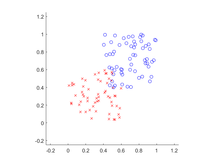
This paper is organized as follows. We introduce some preliminary materials of the SVM in 2​m2​m−1\frac{2m}{2m-1}-norm RKBS in Section 2. Next, we study the splitting method based on ADMM for Optimization (2.1) in Section 3. Moreover, we discuss the global convergence of the iterative algorithm for lower semi-continuous and subanalytic loss function in Section 4. Finally, we give some numerical examples for synthetic data and real data in Section 5 to show that the SVM in RKBS with lower semi-continuous loss function is better than the SVM in RKHS with convex loss function in some cases.

2 Support Vector Machines in 2​m2​m−1\frac{2m}{2m-1}-norm Reproducing Kernel Banach Space

In this section, we review some preliminaries of the SVM in 2​m2​m−1\frac{2m}{2m-1}-norm RKBS. We denote the set of positive integers as ℕ\mathbb{N}, the set of natural numbers as ℕ0\mathbb{N}_{0} and the finite set {1,2,…,N}\{1,2,...,N\} as ℕN\mathbb{N}_{N} respectively. Also, ℕd\mathbb{N}^{d} is the tensor product of positive integers and ℝd\mathbb{R}^{d} is the dd-dimensional Euclidean space. For the rest of this paper, without specification, every vector is supposed to be a column vector.

2.1 2​m2​m−1\frac{2m}{2m-1}-norm Reproducing Kernel Banach Space

For convenient coding and computation, in this subsection, we review the basic concepts of infinite-dimensional 2​m2​m−1\frac{2m}{2m-1}-norm separable RKBS (See [29, Section 3.2]), m∈ℕm\in\mathbb{N}. For a given nonempty subset X⊆ℝdX\subseteq\mathbb{R}^{d} and a linearly independent basis ϕn:X→ℝ,n=1,2,…,\phi_{n}:X\to\mathbb{R},\ n=1,2,..., such that

∑n∈ℕ|ϕn​(𝒙)|<∞​for all​𝒙∈X,\sum_{n\in\mathbb{N}}|\phi_{n}(\boldsymbol{x})|<\infty\ \text{for all}\ \boldsymbol{x}\in X,

we introduce the following 2​m2​m−1\frac{2m}{2m-1}-norm Banach space of continuous functions over XX, that is,

ℬK2​m2​m−1(X):={f:=∑n∈ℕanϕn:an∈ℝ,∑n∈ℕ|an|2​m2​m−1<∞},\mathcal{B}^{\frac{2m}{2m-1}}_{K}(X):=\left\{f:=\sum\limits_{n\in\mathbb{N}}a_{n}\phi_{n}:\ a_{n}\in\mathbb{R},\ \sum_{n\in\mathbb{N}}|a_{n}|^{\frac{2m}{2m-1}}<\infty\right\},

equipped with the norm ‖f‖ℬK2​m2​m−1​(X):=(∑n∈ℕ|an|2​m2​m−1)2​m−12​m\|f\|_{\mathcal{B}^{\frac{2m}{2m-1}}_{K}(X)}:=\left(\sum\limits_{n\in\mathbb{N}}|a_{n}|^{\frac{2m}{2m-1}}\right)^{\frac{2m-1}{2m}} and the well-defined kernel K:X×X→ℝK:X\times X\to\mathbb{R}, and

K⁡(𝒙,𝒙′):=∑n∈ℕϕn​(𝒙)​ϕn​(𝒙′),∀𝒙,𝒙′∈X.K(\boldsymbol{x},\boldsymbol{x}^{\prime}):=\sum\limits_{n\in\mathbb{N}}\phi_{n}(\boldsymbol{x})\phi_{n}(\boldsymbol{x}^{\prime}),\ \forall\boldsymbol{x},\boldsymbol{x}^{\prime}\in X.

Let l2​m2​m−1l^{\frac{2m}{2m-1}} and l2​ml^{2m} be the set of all countable sequences of real scalars with the standard 2​m2​m−1\frac{2m}{2m-1}-norm and 2​m2m-norm, respectively. This construction of ℬK2​m2​m−1​(X)\mathcal{B}^{\frac{2m}{2m-1}}_{K}(X) ensures that ℬK2​m2​m−1​(X)\mathcal{B}^{\frac{2m}{2m-1}}_{K}(X) is isometrically isomorphic to l2​m2​m−1l^{\frac{2m}{2m-1}}, that is, ℬK2​m2​m−1​(X)≅l2​m2​m−1\mathcal{B}^{\frac{2m}{2m-1}}_{K}(X)\cong l^{\frac{2m}{2m-1}}. Let (l2​m2​m−1)′(l^{\frac{2m}{2m-1}})^{{}^{\prime}} and (ℬK2​m2​m−1(X))′(\mathcal{B}^{\frac{2m}{2m-1}}_{K}(X))^{{}^{\prime}} be the dual space of l2​m2​m−1l^{\frac{2m}{2m-1}} and ℬK2​m2​m−1​(X)\mathcal{B}^{\frac{2m}{2m-1}}_{K}(X), respectively. Since (l2​m2​m−1)′≅l2​m(l^{\frac{2m}{2m-1}})^{{}^{\prime}}\cong l^{2m}, we have that

(ℬK2​m2​m−1(X))′≅ℬK2​m(X):={g:=∑n∈ℕbnϕn:bn∈ℝ,∑n∈ℕ|bn|2​m<∞},(\mathcal{B}^{\frac{2m}{2m-1}}_{K}(X))^{{}^{\prime}}\cong\mathcal{B}^{2m}_{K}(X):=\left\{g:=\sum\limits_{n\in\mathbb{N}}b_{n}\phi_{n}:\ b_{n}\in\mathbb{R},\ \sum_{n\in\mathbb{N}}|b_{n}|^{2m}<\infty\right\},

and ℬK2​m​(X)\mathcal{B}^{2m}_{K}(X) is equipped with the norm ‖g‖ℬK2​m​(X):=(∑n∈ℕ|bn|2​m)12​m\|g\|_{\mathcal{B}^{2m}_{K}(X)}:=\left(\sum\limits_{n\in\mathbb{N}}|b_{n}|^{2m}\right)^{\frac{1}{2m}} and the same kernel KK. Moreover, we find that the dual bilinear product of ℬK2​m2​m−1​(X)\mathcal{B}^{\frac{2m}{2m-1}}_{K}(X) is consistent with the dual bilinear product of l2​m2​m−1l^{\frac{2m}{2m-1}}, that is,

⟨f,g⟩ℬK2​m2​m−1​(X)=⟨{an},{bn}⟩l2​m2​m−1=∑n∈ℕan​bn,\langle f,g\rangle_{\mathcal{B}^{\frac{2m}{2m-1}}_{K}(X)}=\langle\{a_{n}\},\{b_{n}\}\rangle_{l^{\frac{2m}{2m-1}}}=\sum\limits_{n\in\mathbb{N}}a_{n}b_{n},

for all f∈ℬK2​m2​m−1​(X)f\in\mathcal{B}^{\frac{2m}{2m-1}}_{K}(X) and g∈ℬK2​m​(X)g\in\mathcal{B}^{2m}_{K}(X). Next we check the two-sided reproducing property of ℬK2​m2​m−1​(X)\mathcal{B}^{\frac{2m}{2m-1}}_{K}(X), that is, for all 𝒙,𝒙′∈X\boldsymbol{x},\boldsymbol{x}^{\prime}\in X, f∈ℬK2​m2​m−1​(X)f\in\mathcal{B}^{\frac{2m}{2m-1}}_{K}(X), g∈ℬK2​m​(X)g\in\mathcal{B}^{2m}_{K}(X),

K⁡(𝒙,⋅)=∑n∈ℕϕn​(𝒙)​ϕn∈ℬK2​m​(X),⟨f,K⁡(𝒙,⋅)⟩ℬK2​m2​m−1​(X)=∑n∈ℕan​ϕn​(𝒙)=f⁡(𝒙),K(\boldsymbol{x},\cdot)=\sum_{n\in\mathbb{N}}\phi_{n}(\boldsymbol{x})\phi_{n}\in\mathcal{B}^{2m}_{K}(X),\ \ \langle f,K(\boldsymbol{x},\cdot)\rangle_{\mathcal{B}^{\frac{2m}{2m-1}}_{K}(X)}=\sum_{n\in\mathbb{N}}a_{n}\phi_{n}(\boldsymbol{x})=f(\boldsymbol{x}),

and

K⁡(⋅,𝒙′)=∑n∈ℕϕn​(𝒙′)​ϕn∈ℬK2​m2​m−1​(X),⟨K⁡(⋅,𝒙′),g⟩ℬK2​m2​m−1​(X)=∑n∈ℕbn​ϕn​(𝒙′)=g⁡(𝒙′).K(\cdot,\boldsymbol{x}^{\prime})=\sum_{n\in\mathbb{N}}\phi_{n}(\boldsymbol{x}^{\prime})\phi_{n}\in\mathcal{B}^{\frac{2m}{2m-1}}_{K}(X),\ \ \langle K(\cdot,\boldsymbol{x}^{\prime}),g\rangle_{\mathcal{B}^{\frac{2m}{2m-1}}_{K}(X)}=\sum_{n\in\mathbb{N}}b_{n}\phi_{n}(\boldsymbol{x}^{\prime})=g(\boldsymbol{x}^{\prime}).

Specially, for any m∈ℕm\in\mathbb{N}, ℬK2​m2​m−1​(X)\mathcal{B}^{\frac{2m}{2m-1}}_{K}(X) has the same reproducing kernel KK. In particular, when m=1m=1, 2​m2​m−1=2\frac{2m}{2m-1}=2 and ℬK2​(X)\mathcal{B}_{K}^{2}(X) is consistent with the separable RKHS.

2.2 Support Vector Machines in 2​m2​m−1\frac{2m}{2m-1}-norm Reproducing Kernel Banach Space

In this subsection, we introduce some preliminaries of the SVM in ℬK2​m2​m−1​(X)\mathcal{B}^{\frac{2m}{2m-1}}_{K}(X). Let XX and YY be the sample space in ℝd\mathbb{R}^{d} and the label space in ℝ\mathbb{R}, respectively. We have the training data

D:={(𝒙i,yi):i=1,2,…,N}⊆X×Y,D:=\{(\boldsymbol{x}_{i},y_{i}):i=1,2,...,N\}\subseteq X\times Y,

composed of input data 𝒙1,𝒙2,…,𝒙N∈X\boldsymbol{x}_{1},\boldsymbol{x}_{2},...,\boldsymbol{x}_{N}\in X and output data y1,y2,…,yN∈Yy_{1},y_{2},...,y_{N}\in Y. To avoid overfitting, we use the training data DD to learn a function fD:X→ℝf_{D}:X\to\mathbb{R} that achieves the smallest regularized possible empirical risk in a given kernel-based function space over XX and build the corresponding SVM ℛ​fD:X→Y\mathcal{R}f_{D}:X\to Y to predict the label of 𝒙≠𝒙i,i=1,2,…,N\boldsymbol{x}\neq\boldsymbol{x}_{i},\ i=1,2,...,N. According to the task requirements, we use fDf_{D} to construct different SVMs. For example, if Y=ℝY=\mathbb{R}, then we build ℛ​fD=fD\mathcal{R}f_{D}=f_{D} for regression. If Y={+1,−1}Y=\{+1,-1\}, then we can build the following SVM

ℛ​fD​(𝒙)={+1,fD​(𝒙)≥0,−1,fD​(𝒙)<0.\mathcal{R}f_{D}(\boldsymbol{x})=\begin{cases}+1,&f_{D}(\boldsymbol{x})\geq 0,\\ -1,&f_{D}(\boldsymbol{x})<0.\end{cases}

for binary classification (See [26, Section 8 and 9]). The classical SVM is discussed in a dd-dimensional RKHS consisting all linear functionals on XX with linear kernel (see [8] and [26, Section 1.3]). For more flexible kernels such as those of Gaussian kernels, which belong to the most important kernels in practice, the corresponding RKHS is infinite-dimensional such that the learning algorithms can be chosen from the enough large amounts of suitable solutions (see in [26, Chapter 5]). The SVM in RKHS has two main areas of application: risk minimization in machine learning and data mining. The typical examples of the SVM in RKHS are the price assessment of a house based on certain characteristics for regression and the automatic recognition of hand-written digits for classification. After the success of the SVM in RKHS, people begin to discuss the SVM in RKBS because RKHS is a special case of RKBS.

Since ℬK2​(X)\mathcal{B}_{K}^{2}(X) is a separable RKHS with reproducing kernel KK, the SVM in ℬK2​(X)\mathcal{B}_{K}^{2}(X) is consistent with the SVM in separable RKHS. Recently, [29, Section 5.4] generalizes the SVM in ℬK2​(X)\mathcal{B}_{K}^{2}(X) to ℬK2​m2​m−1​(X)\mathcal{B}^{\frac{2m}{2m-1}}_{K}(X). For a given ℬK2​m2​m−1​(X)\mathcal{B}^{\frac{2m}{2m-1}}_{K}(X), the training data DD and λ>0\lambda>0, we will find a function in ℬK2​m2​m−1​(X)\mathcal{B}^{\frac{2m}{2m-1}}_{K}(X) that achieves the smallest regularized possible empirical risk, that is,

inff∈ℬK2​m2​m−1​(X)1N​∑i∈ℕNL⁡(𝒙i,yi,f⁡(𝒙i))+λ​‖f‖ℬK2​m2​m−1​(X)2​m2​m−1,\mathop{\mathrm{inf}}_{f\in\mathcal{B}^{\frac{2m}{2m-1}}_{K}(X)}\ \frac{1}{N}\sum_{i\in\mathbb{N}_{N}}L(\boldsymbol{x}_{i},y_{i},f(\boldsymbol{x}_{i}))+\lambda\|f\|_{\mathcal{B}^{\frac{2m}{2m-1}}_{K}(X)}^{\frac{2m}{2m-1}}, (2.1)

where L:X×Y×ℝ→[0,∞)L:X\times Y\times\mathbb{R}\rightarrow[0,\infty) is a given loss function and λ​‖f‖ℬK2​m2​m−1​(X)2​m2​m−1\lambda\|f\|_{\mathcal{B}^{\frac{2m}{2m-1}}_{K}(X)}^{\frac{2m}{2m-1}} is the regularization term used to penalize ff with the large RKBS norm. In the following, we will interpret L⁡(𝒙,y,f⁡(𝒙))L(\boldsymbol{x},y,f(\boldsymbol{x})) as the loss of predicting yy by f⁡(𝒙)f(\boldsymbol{x}) if 𝒙\boldsymbol{x} is observed, that is, the smaller the value L⁡(𝒙,y,f⁡(𝒙))L(\boldsymbol{x},y,f(\boldsymbol{x})) is, the better f⁡(𝒙)f(\boldsymbol{x}) predicts yy in the sense of LL (See Section 5 for more detail). It is clear that Optimization (2.1) is infinite-dimensional and nonnegative. We denote the minimizer of Optimization (2.1) as fD2​m2​m−1f_{D}^{\frac{2m}{2m-1}}, then we build the SVM ℛ​fD2​m2​m−1:X→Y\mathcal{R}f_{D}^{\frac{2m}{2m-1}}:X\to Y according to the task requirement. Moreover, SVMs constructed by different minimizers of Optimization (2.1) have no difference in performance. Hence, we just need to find a minimizer of Optimization (2.1). Next, we focus on the minimizer of Optimization (2.1).

2.3 Duality Mapping and Tensor

To discuss the minimizer of Optimization (2.1), we review some concepts of duality mapping and tensor in ℬK2​m2​m−1​(X)\mathcal{B}^{\frac{2m}{2m-1}}_{K}(X) (See [27, Section 2.1] and [31, Section 3]). Recall that a mapping (not necessarily linear) ΨK2​m2​m−1:ℬK2​m2​m−1​(X)→ℬK2​m​(X)\Psi_{K}^{\frac{2m}{2m-1}}:\mathcal{B}^{\frac{2m}{2m-1}}_{K}(X)\to\mathcal{B}^{2m}_{K}(X) is called duality mapping if

‖ΨK2​m2​m−1​(f)‖ℬK2​m​(X)=‖f‖ℬK2​m2​m−1​(X)12​m−1​and​⟨f,ΨK2​m2​m−1​(f)⟩ℬK2​m2​m−1​(X)=‖f‖ℬK2​m2​m−1​(X)2​m2​m−1.\|\Psi_{K}^{\frac{2m}{2m-1}}(f)\|_{\mathcal{B}^{2m}_{K}(X)}=\|f\|_{\mathcal{B}^{\frac{2m}{2m-1}}_{K}(X)}^{\frac{1}{2m-1}}\ \text{and}\ \langle f,\Psi_{K}^{\frac{2m}{2m-1}}(f)\rangle_{\mathcal{B}^{\frac{2m}{2m-1}}_{K}(X)}=\|f\|_{\mathcal{B}^{\frac{2m}{2m-1}}_{K}(X)}^{\frac{2m}{2m-1}}.

Since l2​m2​m−1l^{\frac{2m}{2m-1}} is reflexive, strictly convex and smooth, ℬK2​m2​m−1​(X)\mathcal{B}^{\frac{2m}{2m-1}}_{K}(X) is also reflexive, strictly convex and smooth. Hence, ΨK2​m2​m−1\Psi_{K}^{\frac{2m}{2m-1}} is a homeomorphism, and

ΨK2​m2​m−1​(f)\displaystyle\Psi_{K}^{\frac{2m}{2m-1}}(f) =∑n∈ℕ(an)12​m−1​ϕn,∀f∈ℬK2​m2​m−1​(X),\displaystyle=\sum_{n\in\mathbb{N}}(a_{n})^{\frac{1}{2m-1}}\phi_{n},\ \forall f\in\mathcal{B}^{\frac{2m}{2m-1}}_{K}(X),
(ΨK2​m2​m−1)−1​(g)\displaystyle(\Psi_{K}^{\frac{2m}{2m-1}})^{-1}(g) =∑n∈ℕ(bn)2​m−1​ϕn,∀g∈ℬK2​m​(X).\displaystyle=\sum\limits_{n\in\mathbb{N}}(b_{n})^{2m-1}\phi_{n},\ \forall g\in\mathcal{B}^{2m}_{K}(X).

If m=1m=1, then ΨK2\Psi_{K}^{2} is an identity mapping and thus linear from ℬK2​(X)\mathcal{B}_{K}^{2}(X) onto ℬK2​(X)\mathcal{B}_{K}^{2}(X). However, if m>1m>1, then ΨK2​m2​m−1\Psi_{K}^{\frac{2m}{2m-1}} is nonlinear but continuous. Furthermore, we obtain the following formula of Fréchet derivative (see the proof of [29, Theorem 5.2])

∇(∥⋅∥ℬK2​m2​m−1​(X))(f)=ΨK2​m2​m−1​(f)‖f‖ℬK2​m2​m−1​(X)12​m−1∈ℬK2​m(X),∀f≠0,\nabla(\|\cdot\|_{\mathcal{B}^{\frac{2m}{2m-1}}_{K}(X)})(f)=\frac{\Psi_{K}^{\frac{2m}{2m-1}}(f)}{\|f\|_{\mathcal{B}^{\frac{2m}{2m-1}}_{K}(X)}^{\frac{1}{2m-1}}}\in\mathcal{B}^{2m}_{K}(X),\ \ \forall f\neq 0, (2.2)

where ∇\nabla denotes the Fréchet derivative. In particular, for a differentiable real function, ∇\nabla represents the gradient and ∇2\nabla^{2} represents the Hessian matrix, respectively.

Next we review some basic theory of tensor in ℬK2​m2​m−1​(X)\mathcal{B}^{\frac{2m}{2m-1}}_{K}(X). For convenience of readers, the notations and operations of tensors are defined as in the book [21]. For the training data DD, let

𝚽n:=(ϕn(𝒙1),ϕn(𝒙2),..,ϕn(𝒙N))T∈ℝN,n∈ℕ.\boldsymbol{\boldsymbol{\Phi}}_{n}:=\left(\phi_{n}(\boldsymbol{x}_{1}),\phi_{n}(\boldsymbol{x}_{2}),..,\phi_{n}(\boldsymbol{x}_{N})\right)^{T}\in\mathbb{R}^{N},\ n\in\mathbb{N}.

Since 2​m2m is even, we define the following (2​m)(2m)-th order NN-dimensional real tensor in ℬK2​m2​m−1​(X)\mathcal{B}^{\frac{2m}{2m-1}}_{K}(X)

𝒜K2​m:=(∑n∈ℕϕn​(𝒙i1)​ϕn​(𝒙i2)​…​ϕn​(𝒙i2​m))i1,i2,…,i2​m=1N,N,…,N=∑n∈ℕ(𝚽n)⊗2​m,\mathcal{A}_{K}^{2m}:=\left(\sum\limits_{n\in\mathbb{N}}\phi_{n}(\boldsymbol{x}_{i_{1}})\phi_{n}(\boldsymbol{x}_{i_{2}})...\phi_{n}(\boldsymbol{x}_{i_{2m}})\right)_{i_{1},i_{2},...,i_{2m}=1}^{N,N,...,N}=\sum\limits_{n\in\mathbb{N}}(\boldsymbol{\Phi}_{n})^{\otimes 2m},

where ⊗\otimes denotes the tensor outer product. Specially, if m=1m=1, then 𝒜K2\mathcal{A}_{K}^{2} is a matrix in ℬK2​(X)\mathcal{B}_{K}^{2}(X). It is easy to check that 𝒜K2​m\mathcal{A}_{K}^{2m} is symmetric, that is, all entries of 𝒜K2​m\mathcal{A}_{K}^{2m} are invariant under any permutation of the indices. For any 𝒄∈ℝN\boldsymbol{c}\in\mathbb{R}^{N}, we denote

𝒜K2​m​𝒄2​m:=\displaystyle\mathcal{A}_{K}^{2m}\boldsymbol{c}^{2m}:= (∑n∈ℕ(𝚽n)⊗2​m)⋅𝒄⊗2​m=∑n∈ℕ(𝚽nT​𝒄)2​m≥0,\displaystyle\left(\sum\limits_{n\in\mathbb{N}}(\boldsymbol{\Phi}_{n})^{\otimes 2m}\right)\cdot\boldsymbol{c}^{\otimes 2m}=\sum_{n\in\mathbb{N}}\left(\boldsymbol{\Phi}_{n}^{T}\boldsymbol{c}\right)^{2m}\geq 0,
𝒜K2​m​𝒄2​m−1:=\displaystyle\mathcal{A}_{K}^{2m}\boldsymbol{c}^{2m-1}:= (∑n∈ℕ(𝚽n)⊗2​m)⋅𝒄⊗2​m−1=∑n∈ℕ(𝚽nT​𝒄)2​m−1​𝚽n∈ℝN,\displaystyle\left(\sum\limits_{n\in\mathbb{N}}(\boldsymbol{\Phi}_{n})^{\otimes 2m}\right)\cdot\boldsymbol{c}^{\otimes 2m-1}=\sum_{n\in\mathbb{N}}\left(\boldsymbol{\Phi}_{n}^{T}\boldsymbol{c}\right)^{2m-1}\boldsymbol{\Phi}_{n}\in\mathbb{R}^{N},
𝒜K2​m​𝒄2​m−2:=\displaystyle\mathcal{A}_{K}^{2m}\boldsymbol{c}^{2m-2}:= (∑n∈ℕ(𝚽n)⊗2​m)⋅𝒄⊗2​m−2=∑n∈ℕ(𝚽nT​𝒄)2​m−2​𝚽n​𝚽nT∈ℝN×N.\displaystyle\left(\sum\limits_{n\in\mathbb{N}}(\boldsymbol{\Phi}_{n})^{\otimes 2m}\right)\cdot\boldsymbol{c}^{\otimes 2m-2}=\sum_{n\in\mathbb{N}}\left(\boldsymbol{\Phi}_{n}^{T}\boldsymbol{c}\right)^{2m-2}\boldsymbol{\Phi}_{n}\boldsymbol{\Phi}_{n}^{T}\in\mathbb{R}^{N\times N}.

Specially, we adopt the convention that 𝒜K2​𝒄0=𝒜K2\mathcal{A}_{K}^{2}\boldsymbol{c}^{0}=\mathcal{A}_{K}^{2} for any 𝒄≠𝟎\boldsymbol{c}\neq\boldsymbol{0}. It is clear that

𝒜K2​m​𝒄2​m=(𝒜K2​m​𝒄2​m−1)T​𝒄,𝒜K2​m​𝒄2​m−1=𝒜K2​m​𝒄2​m−2⋅𝒄.\mathcal{A}_{K}^{2m}\boldsymbol{c}^{2m}=(\mathcal{A}_{K}^{2m}\boldsymbol{c}^{2m-1})^{T}\boldsymbol{c},\ \ \mathcal{A}_{K}^{2m}\boldsymbol{c}^{2m-1}=\mathcal{A}_{K}^{2m}\boldsymbol{c}^{2m-2}\cdot\boldsymbol{c}. (2.3)

Also, by derivative rule, we have that for any 𝒄∈ℝN\boldsymbol{c}\in\mathbb{R}^{N},

∇(𝒜K2​m​(⋅)2​m)​(𝒄)=2​m​𝒜K2​m​𝒄2​m−1,∇2(𝒜K2​m​(⋅)2​m)​(𝒄)=2​m​(2​m−1)​𝒜K2​m​𝒄2​m−2.\nabla(\mathcal{A}_{K}^{2m}(\cdot)^{2m})(\boldsymbol{c})=2m\mathcal{A}_{K}^{2m}\boldsymbol{c}^{2m-1},\ \ \nabla^{2}(\mathcal{A}_{K}^{2m}(\cdot)^{2m})(\boldsymbol{c})=2m(2m-1)\mathcal{A}_{K}^{2m}\boldsymbol{c}^{2m-2}. (2.4)

By definition, it is easy to check that 𝒜K2​m​𝒄2​m−2\mathcal{A}_{K}^{2m}\boldsymbol{c}^{2m-2} is symmetric. For any 𝒅∈ℝN\boldsymbol{d}\in\mathbb{R}^{N}, we have that

𝒅T​(𝒜K2​m​𝒄2​m−2)​𝒅=∑n∈ℕ(𝚽nT​𝒄)2​m−2​(𝚽nT​𝒅)2≥0.\boldsymbol{d}^{T}\left(\mathcal{A}_{K}^{2m}\boldsymbol{c}^{2m-2}\right)\boldsymbol{d}=\sum_{n\in\mathbb{N}}\left(\boldsymbol{\Phi}_{n}^{T}\boldsymbol{c}\right)^{2m-2}\left(\boldsymbol{\Phi}_{n}^{T}\boldsymbol{d}\right)^{2}\geq 0.

Thus, 𝒜K2​m​𝒄2​m−2\mathcal{A}_{K}^{2m}\boldsymbol{c}^{2m-2} is a positive definite matrix.

2.4 Representer Theorem

The loss functions and RKBSs are the core research content, because it determines the minimizer of Optimization (2.1). For machine learning, the most common loss function is convex loss function, that is, L(𝒙,y,⋅)L(\boldsymbol{x},y,\cdot) is a convex function for all 𝒙∈X\boldsymbol{x}\in X and y∈Yy\in Y. Besides convexity, we can define other loss functions in a similar way, such as continuity, smoothness, lower semi-continuity, etc. Specially, if LL is a convex loss function, then LL is a lower semi-continuous loss function. But the lower semi-continuity can not imply the convexity.

If LL is a convex loss function, then [29, Theorem 5.2] assures that Optimization (2.1) in ℬK2​m2​m−1​(X)\mathcal{B}^{\frac{2m}{2m-1}}_{K}(X) with convex loss function has a unique minimizer contained in a known finite-dimensional space spanned by the reproducing kernel KK and the training data DD, even if the space ℬK2​m2​m−1​(X)\mathcal{B}^{\frac{2m}{2m-1}}_{K}(X) itself is substantially larger. The convex loss function is viewed as highly preferable in many publications because of their computational advantages (unique minimizer, ease-of-use, ability to be efficiently optimized by convex optimization tools, etc.).

Recently, some nonconvex and lower semi-continuous loss functions, such as ramp loss and truncated pinball loss are proposed and used in SVM (see [7, 11, 16, 24]). From some preliminary numerical experiments in [29, Chapter 6], it shows that the SVM in ℬK43​(X)\mathcal{B}_{K}^{\frac{4}{3}}(X) may perform better than the SVM in ℬK2​(X)\mathcal{B}_{K}^{2}(X) with Hinge loss and Gaussian kernel in some cases. Furthermore, the SVM in ℬK65​(X)\mathcal{B}_{K}^{\frac{6}{5}}(X) may perform better than the SVM in ℬK43​(X)\mathcal{B}_{K}^{\frac{4}{3}}(X) and ℬK2​(X)\mathcal{B}_{K}^{2}(X) with a nonconvex linear piecewise loss function and Gaussian kernel in some cases (See Section 5). But an effective algorithm for the SVM in ℬK2​m2​m−1​(X)\mathcal{B}^{\frac{2m}{2m-1}}_{K}(X) with lower semi-continuous loss function is still lack of study. Thus, in the rest of this paper, we mainly study how to solve Optimization (2.1) in ℬK2​m2​m−1​(X)\mathcal{B}^{\frac{2m}{2m-1}}_{K}(X) with lower semi-continuous loss function. First, we establish the representer theorem by the same techniques as those used in [13]. We present it below.

Lemma 2.1.

If LL is a lower semi-continuous loss function, then Optimization (2.1) has a minimizer fD2​m2​m−1f_{D}^{\frac{2m}{2m-1}} such that

fD2​m2​m−1∈ΔK2​m2​m−1​(X):=(ΨK2​m2​m−1)−1​(span⁡{K⁡(𝒙1,⋅),…,K⁡(𝒙N,⋅)}).f_{D}^{\frac{2m}{2m-1}}\in\Delta_{K}^{\frac{2m}{2m-1}}(X):=(\Psi_{K}^{\frac{2m}{2m-1}})^{-1}(\mathrm{span}\{K(\boldsymbol{x}_{1},\cdot),...,K(\boldsymbol{x}_{N},\cdot)\}).
Proof.

From (2.1), ℬK2​m2​m−1​(X)\mathcal{B}^{\frac{2m}{2m-1}}_{K}(X) is a two-sided RKBS and thus a right-sided RKBS (See [29, Definition 2.1]). By [9, Definition 2.2.27] and reflexity of ℬK2​m2​m−1​(X)\mathcal{B}^{\frac{2m}{2m-1}}_{K}(X), the predual space of ℬK2​m2​m−1​(X)\mathcal{B}^{\frac{2m}{2m-1}}_{K}(X) is ℬK2​m​(X)\mathcal{B}^{2m}_{K}(X). Moreover, the right-sided reproducing property of ℬK2​m2​m−1​(X)\mathcal{B}^{\frac{2m}{2m-1}}_{K}(X) shows that {K⁡(𝒙,⋅):𝒙∈X}⊆ℬK2​m​(X)\{K(\boldsymbol{x},\cdot):\boldsymbol{x}\in X\}\subseteq\mathcal{B}^{2m}_{K}(X). In conclusion, we use λ∥⋅∥ℬK2​m2​m−1​(X)2​m2​m−1\lambda\|\cdot\|_{\mathcal{B}^{\frac{2m}{2m-1}}_{K}(X)}^{\frac{2m}{2m-1}} instead of λ∥⋅∥ℬK2​m2​m−1​(X)2\lambda\|\cdot\|_{\mathcal{B}^{\frac{2m}{2m-1}}_{K}(X)}^{2} to reproof [13, Theorem 3.1] and use similar line of arguments of [13, Corollary 4.1] to show that Optimization (2.1) has a minimizer fD2​m2​m−1f_{D}^{\frac{2m}{2m-1}}. Moreover, if fD2​m2​m−1≠0f_{D}^{\frac{2m}{2m-1}}\neq 0, then (2.2) guarantees that

ΨK2​m2​m−1​(fD2​m2​m−1)‖fD2​m2​m−1‖ℬK2​m2​m−1​(X)12​m−1=∇(∥⋅∥ℬK2​m2​m−1​(X))(fD2​m2​m−1)∈span{K(𝒙1,⋅),…,K(𝒙N,⋅)},\frac{\Psi_{K}^{\frac{2m}{2m-1}}(f_{D}^{\frac{2m}{2m-1}})}{\|f_{D}^{\frac{2m}{2m-1}}\|_{\mathcal{B}^{\frac{2m}{2m-1}}_{K}(X)}^{\frac{1}{2m-1}}}=\nabla(\|\cdot\|_{\mathcal{B}^{\frac{2m}{2m-1}}_{K}(X)})(f_{D}^{\frac{2m}{2m-1}})\in\mathrm{span}\{K(\boldsymbol{x}_{1},\cdot),...,K(\boldsymbol{x}_{N},\cdot)\},

which ensures that

fD2​m2​m−1∈ΔK2​m2​m−1​(X)=(ΨK2​m2​m−1)−1​(span⁡{K⁡(𝒙1,⋅),…,K⁡(𝒙N,⋅)}).f_{D}^{\frac{2m}{2m-1}}\in\Delta_{K}^{\frac{2m}{2m-1}}(X)=(\Psi_{K}^{\frac{2m}{2m-1}})^{-1}(\mathrm{span}\{K(\boldsymbol{x}_{1},\cdot),...,K(\boldsymbol{x}_{N},\cdot)\}).

If fD2​m2​m−1=0f_{D}^{\frac{2m}{2m-1}}=0, then the proof is straight-forward. This completes the proof. ∎

Since ΨK2​m2​m−1\Psi_{K}^{\frac{2m}{2m-1}} is a homeomorphism and span⁡{K⁡(𝒙1,⋅),…,K⁡(𝒙N,⋅)}\mathrm{span}\{K(\boldsymbol{x}_{1},\cdot),...,K(\boldsymbol{x}_{N},\cdot)\} is a finite-dimensional subspace and thus a closed subset in ℬK2​m​(X)\mathcal{B}^{2m}_{K}(X), ΔK2​m2​m−1​(X)\Delta_{K}^{\frac{2m}{2m-1}}(X) is a closed subset in ℬK2​m2​m−1​(X)\mathcal{B}^{\frac{2m}{2m-1}}_{K}(X). If m=1m=1, then ΨK2\Psi_{K}^{2} is linear and ΔK2​(X)\Delta_{K}^{2}(X) is a subspace. If m>1m>1, then ΨK2​m2​m−1\Psi_{K}^{\frac{2m}{2m-1}} is nonlinear and ΔK2​m2​m−1​(X)\Delta_{K}^{\frac{2m}{2m-1}}(X) is not a subspace.

Remark 2.2.

If LL is a lower semi-continuous and nonconvex loss function, then Optimization (2.1) may have more than one minimizer and at least one of them is in ΔK2​m2​m−1​(X)\Delta_{K}^{\frac{2m}{2m-1}}(X). Hence, we focus on finding the minimizer in ΔK2​m2​m−1​(X)\Delta_{K}^{\frac{2m}{2m-1}}(X).

2.5 Tensor Optimization

In this subsection, we introduce how to equivalently transfer Optimization (2.1) to a finite-dimensional tensor Optimization. First, Lemma 2.1 shows that Optimization (2.1) in ℬK2​m2​m−1​(X)\mathcal{B}^{\frac{2m}{2m-1}}_{K}(X) can be equivalently transferred to Optimization (2.1) in ΔK2​m2​m−1​(X)\Delta_{K}^{\frac{2m}{2m-1}}(X). For any f∈ΔK2​m2​m−1​(X)f\in\Delta_{K}^{\frac{2m}{2m-1}}(X), there exists a vector 𝒄=(c1,c2​…,cN)T∈ℝN\boldsymbol{c}=(c_{1},c_{2}...,c_{N})^{T}\in\mathbb{R}^{N} such that

ΨK2​m2​m−1​(f)=∑i∈ℕNci​K​(𝒙i,⋅)=∑n∈ℕ(𝚽nT​𝒄)​ϕn.\Psi_{K}^{\frac{2m}{2m-1}}(f)=\sum_{i\in\mathbb{N}_{N}}c_{i}K(\boldsymbol{x}_{i},\cdot)=\sum_{n\in\mathbb{N}}\left(\boldsymbol{\Phi}_{n}^{T}\boldsymbol{c}\right)\phi_{n}.

Thus, ff has the representation

f=(ΨK2​m2​m−1)−1​(∑n∈ℕ(𝚽nT​𝒄)​ϕn)=∑n∈ℕ(𝚽nT​𝒄)2​m−1​ϕn,f=(\Psi_{K}^{\frac{2m}{2m-1}})^{-1}\left(\sum_{n\in\mathbb{N}}\left(\boldsymbol{\Phi}_{n}^{T}\boldsymbol{c}\right)\phi_{n}\right)=\sum_{n\in\mathbb{N}}\left(\boldsymbol{\Phi}_{n}^{T}\boldsymbol{c}\right)^{2m-1}\phi_{n},

which ensures that

f(𝒙i)=∑n∈ℕ(𝚽nT𝒄)2​m−1ϕn(𝒙i)=(𝒜K2​m𝒄2​m−1)i,i=1,2,…,N.f(\boldsymbol{x}_{i})=\sum_{n\in\mathbb{N}}\left(\boldsymbol{\Phi}_{n}^{T}\boldsymbol{c}\right)^{2m-1}\phi_{n}(\boldsymbol{x}_{i})=(\mathcal{A}_{K}^{2m}\boldsymbol{c}^{2m-1})_{i},\ i=1,2,...,N.

On the other hand, by definition of ∥⋅∥ℬK2​m2​m−1​(X)\|\cdot\|_{\mathcal{B}^{\frac{2m}{2m-1}}_{K}(X)}, for any f∈ΔK2​m2​m−1​(X)f\in\Delta_{K}^{\frac{2m}{2m-1}}(X), we compute

‖f‖ℬK2​m2​m−1​(X)2​m2​m−1=∑n∈ℕ|(𝚽nT​𝒄)2​m−1|2​m2​m−1=∑n∈ℕ(𝚽nT​𝒄)2​m=𝒜K2​m​𝒄2​m.\|f\|_{\mathcal{B}^{\frac{2m}{2m-1}}_{K}(X)}^{\frac{2m}{2m-1}}=\sum_{n\in\mathbb{N}}\left|\left(\boldsymbol{\Phi}_{n}^{T}\boldsymbol{c}\right)^{2m-1}\right|^{\frac{2m}{2m-1}}=\sum_{n\in\mathbb{N}}\left(\boldsymbol{\Phi}_{n}^{T}\boldsymbol{c}\right)^{2m}=\mathcal{A}_{K}^{2m}\boldsymbol{c}^{2m}.

Thus, Optimization (2.1) in ΔK2​m2​m−1​(X)\Delta_{K}^{\frac{2m}{2m-1}}(X) can be equivalently transferred to a tensor Optimization in ℝN\mathbb{R}^{N}

min𝒄∈ℝN⁡1N​∑i∈ℕNL⁡(𝒙i,yi,(𝒜K2​m​𝒄2​m−1)i)+λ​𝒜K2​m​𝒄2​m.\min_{\boldsymbol{c}\in\mathbb{R}^{N}}\ \frac{1}{N}\sum_{i\in\mathbb{N}_{N}}L(\boldsymbol{x}_{i},y_{i},(\mathcal{A}_{K}^{2m}\boldsymbol{c}^{2m-1})_{i})+\lambda\mathcal{A}_{K}^{2m}\boldsymbol{c}^{2m}. (2.5)

Since fD2​m2​m−1∈ΔK2​m2​m−1​(X)f_{D}^{\frac{2m}{2m-1}}\in\Delta_{K}^{\frac{2m}{2m-1}}(X) is a minimizer of Optimization (2.1) in ℬK2​m2​m−1​(X)\mathcal{B}^{\frac{2m}{2m-1}}_{K}(X), there exists 𝒄D2​m2​m−1∈ℝN\boldsymbol{c}_{D}^{\frac{2m}{2m-1}}\in\mathbb{R}^{N} such that

fD2​m2​m−1=∑n∈ℕ(𝚽nT​𝒄D2​m2​m−1)2​m−1​ϕnf_{D}^{\frac{2m}{2m-1}}=\sum_{n\in\mathbb{N}}\left(\boldsymbol{\Phi}_{n}^{T}\boldsymbol{c}_{D}^{\frac{2m}{2m-1}}\right)^{2m-1}\phi_{n}

and 𝒄D2​m2​m−1\boldsymbol{c}_{D}^{\frac{2m}{2m-1}} is a minimizer of Optimization (2.5). This ensures that we employ the finite suitable parameters to reconstruct the SVM in ℬK2​m2​m−1​(X)\mathcal{B}^{\frac{2m}{2m-1}}_{K}(X).

3 Splitting Method for Support Vector Machines in 2​m2​m−1\frac{2m}{2m-1}-norm Reproducing Kernel Banach Space

In this section, we consider to find an algorithm based on Optimization (2.5) to compute Optimization (2.1) easily. At present, we mainly use subgradient method, Lagrange multipliers method and sequential minimal optimization (SMO) to design algorithms for SVM. These classical numerical algorithms are suitable for solving convex and smooth programs. Since 𝒄↦(𝒜K2​m​𝒄2​m−1)i\boldsymbol{c}\mapsto(\mathcal{A}_{K}^{2m}\boldsymbol{c}^{2m-1})_{i} is continuous, the lower semi-continuity of L(𝒙i,yi,⋅)L(\boldsymbol{x}_{i},y_{i},\cdot) guarantees the lower semi-continuity of 𝒄↦L⁡(𝒙i,yi,(𝒜K2​m​𝒄2​m−1)i)\boldsymbol{c}\mapsto L(\boldsymbol{x}_{i},y_{i},(\mathcal{A}_{K}^{2m}\boldsymbol{c}^{2m-1})_{i}) for all i=1,2,…,Ni=1,2,...,N which ensures Optimization (2.5) is lower semi-continuous which maybe nonsmooth or nonconvex. Many classical numerical algorithms are not suitable for Optimization (2.5).

The ADMM algorithm, as one of splitting techniques, can even be used to minimize nonsmooth or nonconvex functions. Also, [28] discuss how to use ADMM for the traditional SVM with 0-1 loss function. For general lower semi-continuous loss functions and kernels, we observe that the subproblems in ADMM for Optimization (2.5) can be splitted into some Optimizations which are then easier to handle. Hence, we will study how to solve Optimization (2.1) by the splitting method based on ADMM.

Remark 3.1.

In the rest of this paper, we assume that the training data DD, loss function LL, RKBS ℬK2​m2​m−1​(X)\mathcal{B}^{\frac{2m}{2m-1}}_{K}(X) and λ>0\lambda>0 in Optimization (2.1) and (2.5) are given, which means that N∈ℕN\in\mathbb{N}, m∈ℕm\in\mathbb{N} and the tensor 𝒜K2​m\mathcal{A}_{K}^{2m} are confirmed before algorithm discussion.

For notational convenience, let

F⁡(𝜶):=1N​∑i∈ℕNL⁡(𝒙i,yi,αi),G⁡(𝒄):=λ​𝒜K2​m​𝒄2​m.F(\boldsymbol{\alpha}):=\frac{1}{N}\sum_{i\in\mathbb{N}_{N}}L(\boldsymbol{x}_{i},y_{i},\alpha_{i}),\ \ G(\boldsymbol{c}):=\lambda\mathcal{A}_{K}^{2m}\boldsymbol{c}^{2m}.

To describe the algorithm, we first reformulate Optimization (2.5) as

min𝒂,𝒄F⁡(𝜶)+G⁡(𝒄),s.t.𝜶=𝒜K2​m​𝒄2​m−1.\begin{array}[]{cl}\displaystyle\min_{\boldsymbol{a},\boldsymbol{c}}&\displaystyle F(\boldsymbol{\alpha})+G(\boldsymbol{c}),\\ \text{s.t.}&\boldsymbol{\alpha}=\mathcal{A}_{K}^{2m}\boldsymbol{c}^{2m-1}.\end{array}

Recall that the augmented Lagrangian function for the above problem is defined as:

ℒβ​(𝜶,𝒄,𝜸):=F⁡(𝜶)+G⁡(𝒄)+𝜸T​(𝜶−𝒜K2​m​𝒄2​m−1)+β2​‖𝜶−𝒜K2​m​𝒄2​m−1‖2,\mathcal{L}_{\beta}(\boldsymbol{\alpha},\boldsymbol{c},\boldsymbol{\gamma}):=F(\boldsymbol{\alpha})+G(\boldsymbol{c})+\boldsymbol{\gamma}^{T}(\boldsymbol{\alpha}-\mathcal{A}_{K}^{2m}\boldsymbol{c}^{2m-1})+\frac{\beta}{2}\|\boldsymbol{\alpha}-\mathcal{A}_{K}^{2m}\boldsymbol{c}^{2m-1}\|^{2},

where the Lagrangian multiplier β>0\beta>0 and ∥⋅∥\|\cdot\| denotes the 22-norm in Euclidean space. The splitting method based on ADMM is then presented as follows. Suppose that the algorithm is initialized at (𝜶0,𝒄0,𝜸0)(\boldsymbol{\alpha}^{0},\boldsymbol{c}^{0},\boldsymbol{\gamma}^{0}), its iterative scheme is

𝜶k+1\displaystyle\boldsymbol{\alpha}_{k+1} ∈argmin𝜶∈ℝNℒβ​(𝜶,𝒄k,𝜸k),\displaystyle\in\mathop{\mathrm{argmin}}_{\boldsymbol{\alpha}\in\mathbb{R}^{N}}\ \mathcal{L}_{\beta}(\boldsymbol{\alpha},\boldsymbol{c}_{k},\boldsymbol{\gamma}_{k}), (S-1)
𝒄k+1\displaystyle\boldsymbol{c}_{k+1} ∈argmin𝒄∈ℝNℒβ​(𝜶k+1,𝒄,𝜸k),\displaystyle\in\mathop{\mathrm{argmin}}_{\boldsymbol{c}\in\mathbb{R}^{N}}\ \mathcal{L}_{\beta}(\boldsymbol{\alpha}_{k+1},\boldsymbol{c},\boldsymbol{\gamma}_{k}), (S-2)
𝜸k+1\displaystyle\boldsymbol{\gamma}_{k+1} :=𝜸k+β⁡(𝜶k+1−𝒜K2​m​(𝒄k+1)2​m−1),\displaystyle:=\boldsymbol{\gamma}_{k}+\beta(\boldsymbol{\alpha}_{k+1}-\mathcal{A}_{K}^{2m}(\boldsymbol{c}_{k+1})^{2m-1}), (S-3)
sk+1\displaystyle s_{k+1} :=∑n∈ℕ(𝚽nT​𝒄k+1)2​m−1​ϕn,\displaystyle:=\sum_{n\in\mathbb{N}}\left(\boldsymbol{\Phi}_{n}^{T}\boldsymbol{c}_{k+1}\right)^{2m-1}\phi_{n}, (S-4)

where k∈ℕ0k\in\mathbb{N}_{0}. Since (S-1) only depends on 𝜶\boldsymbol{\alpha} and (S-2) only depends on 𝒄\boldsymbol{c}, combining the linear and quadratic terms, we equivalently transfer (S-1) and (S-2) to

𝜶k+1\displaystyle\boldsymbol{\alpha}_{k+1} ∈argmin𝜶∈ℝNF⁡(𝜶)+β2​‖𝜶−𝒜K2​m​(𝒄k)2​m−1+1β​𝜸k‖2,\displaystyle\in\mathop{\mathrm{argmin}}_{\boldsymbol{\alpha}\in\mathbb{R}^{N}}\ F(\boldsymbol{\alpha})+\frac{\beta}{2}\|\boldsymbol{\alpha}-\mathcal{A}_{K}^{2m}(\boldsymbol{c}_{k})^{2m-1}+\frac{1}{\beta}\boldsymbol{\gamma}_{k}\|^{2}, (S-1’)
𝒄k+1\displaystyle\boldsymbol{c}_{k+1} ∈argmin𝒄∈ℝNG⁡(𝒄)+β2​‖𝜶k+1−𝒜K2​m​𝒄2​m−1+1β​𝜸k‖2.\displaystyle\in\mathop{\mathrm{argmin}}_{\boldsymbol{c}\in\mathbb{R}^{N}}\ G(\boldsymbol{c})+\frac{\beta}{2}\|\boldsymbol{\alpha}_{k+1}-\mathcal{A}_{K}^{2m}\boldsymbol{c}^{2m-1}+\frac{1}{\beta}\boldsymbol{\gamma}_{k}\|^{2}. (S-2’)

By definition, it is easy to check that (S-1’) is lower semi-continuous and (S-2’) is continuous. Moreover, (S-1’) and (S-2’) are coercive (see [1, Definition 2.13]), Weierstrass Theorem [1, Theorem 2.14] assures that (S-1’) and (S-2’) both have a solution. As a consequence, the splitting method above is well-defined and an infinite iterative sequence {(𝜶k,𝒄k,𝜸k,sk)}\{(\boldsymbol{\alpha}_{k},\boldsymbol{c}_{k},\boldsymbol{\gamma}_{k},s_{k})\} is generated. Also, {sk}\{s_{k}\} can be seen as an infinite iterative sequence to approximate the minimizer of Optimization (2.1).

Next, we discuss how to solve subproblems (S-1’) and (S-2’). As for (S-1’), since FF and ∥⋅∥2\|\cdot\|^{2} can be split of the variable into subvectors, we equivalently transfer an Optimization in ℝN\mathbb{R}^{N} to some Optimizations in ℝ\mathbb{R}, that is, for i=1,…,Ni=1,...,N,

(𝜶k+1)i∈argminαiL⁡(𝒙i,yi,αi)N+β2​(αi−(𝒜K2​m​(𝒄k)2​m−1)i+1β​(𝜸k)i)2.(\boldsymbol{\alpha}_{k+1})_{i}\in\mathop{\mathrm{argmin}}_{\alpha_{i}}\ \frac{L(\boldsymbol{x}_{i},y_{i},\alpha_{i})}{N}+\frac{\beta}{2}\left(\alpha_{i}-(\mathcal{A}_{K}^{2m}(\boldsymbol{c}_{k})^{2m-1})_{i}+\frac{1}{\beta}(\boldsymbol{\gamma}_{k})_{i}\right)^{2}. (S-1”)

In other words, we solve Optimization (S-1’) in ℝN\mathbb{R}^{N} by breaking it into NN Optimizations (S-1”) in ℝ\mathbb{R}, each of them easier to handle. For the general lower semi-continuous loss function LL, the minimizer set of (S-1”) may not be a singleton. In this case, we choose one of the elements in the minimizer set as (𝜶k+1)i,i=1,2,…,N(\boldsymbol{\alpha}_{k+1})_{i},\ i=1,2,...,N.

As for (S-2’), it is easy to see that (S-2’) is nonconvex and continuously differentiable. By definition of (S-2’), (2.3) and (2.4), we have

∇(G+β2​‖𝜶k+1−𝒜K2​m​(⋅)2​m−1+1β​𝜸k‖2)​(𝒄)\displaystyle\nabla(G+\frac{\beta}{2}\|\boldsymbol{\alpha}_{k+1}-\mathcal{A}_{K}^{2m}(\cdot)^{2m-1}+\frac{1}{\beta}\boldsymbol{\gamma}_{k}\|^{2})(\boldsymbol{c})
=\displaystyle= 2​m​λ​𝒜K2​m​𝒄2​m−1−β⁡(2​m−1)​𝒜K2​m​𝒄2​m−2⋅(𝜶k+1−𝒜K2​m​𝒄2​m−1+1β​𝜸k)\displaystyle 2m\lambda\mathcal{A}_{K}^{2m}\boldsymbol{c}^{2m-1}-\beta(2m-1)\mathcal{A}_{K}^{2m}\boldsymbol{c}^{2m-2}\cdot(\boldsymbol{\alpha}_{k+1}-\mathcal{A}_{K}^{2m}\boldsymbol{c}^{2m-1}+\frac{1}{\beta}\boldsymbol{\gamma}_{k})
=\displaystyle= β⁡(2​m−1)​𝒜K2​m​𝒄2​m−2⋅(𝒜K2​m​𝒄2​m−1+2​m​λ(2​m−1)​β​𝒄−(𝜶k+1+1β​𝜸k)).\displaystyle\beta(2m-1)\mathcal{A}_{K}^{2m}\boldsymbol{c}^{2m-2}\cdot\left(\mathcal{A}_{K}^{2m}\boldsymbol{c}^{2m-1}+\frac{2m\lambda}{(2m-1)\beta}\boldsymbol{c}-(\boldsymbol{\alpha}_{k+1}+\frac{1}{\beta}\boldsymbol{\gamma}_{k})\right).

Next we show that the solution of the following tensor equation

𝒜K2​m​𝒄2​m−1+2​m​λ(2​m−1)​β​𝒄=𝜶k+1+1β​𝜸k.\mathcal{A}_{K}^{2m}\boldsymbol{c}^{2m-1}+\frac{2m\lambda}{(2m-1)\beta}\boldsymbol{c}=\boldsymbol{\alpha}_{k+1}+\frac{1}{\beta}\boldsymbol{\gamma}_{k}. (S-2”)

is a minimizer of (S-2’) by comparing the function values. We denote

H⁡(𝒄):=12​m​𝒜K2​m​𝒄2​m+m​λ(2​m−1)​β​‖𝒄‖2−(𝜶k+1+1β​𝜸k)T​𝒄.H(\boldsymbol{c}):=\frac{1}{2m}\mathcal{A}_{K}^{2m}\boldsymbol{c}^{2m}+\frac{m\lambda}{(2m-1)\beta}\|\boldsymbol{c}\|^{2}-(\boldsymbol{\alpha}_{k+1}+\frac{1}{\beta}\boldsymbol{\gamma}_{k})^{T}\boldsymbol{c}.

Then the solution of (S-2”) is a stationary point of HH. Also, (2.4) shows that

∇2H​(𝒄)=(2​m−1)​𝒜K2​m​𝒄2​m−2+2​m​λ(2​m−1)​β​I,∀𝒄∈ℝN,\nabla^{2}H(\boldsymbol{c})=(2m-1)\mathcal{A}_{K}^{2m}\boldsymbol{c}^{2m-2}+\frac{2m\lambda}{(2m-1)\beta}I,\ \forall\boldsymbol{c}\in\mathbb{R}^{N},

where II denotes the identity matrix of NN-dimensional. Since 𝒜K2​m​𝒄2​m−2\mathcal{A}_{K}^{2m}\boldsymbol{c}^{2m-2} is symmetric and positive definite, [2, Proposition 1.1.10 (ii)] guarantees that HH is strictly convex on ℝN\mathbb{R}^{N}, which ensures that (S-2”) has a unique solution 𝒄¯\bar{\boldsymbol{c}}. By (S-2”), (2.3) and (2.4), it follows that for any 𝒄∈ℝN\boldsymbol{c}\in\mathbb{R}^{N},

G⁡(𝒄)+β2​‖𝜶k+1−𝒜K2​m​𝒄2​m−1+1β​𝜸k‖2−G⁡(𝒄¯)−β2​‖𝜶k+1−𝒜K2​m​𝒄¯2​m−1+1β​𝜸k‖2\displaystyle G(\boldsymbol{\boldsymbol{c}})+\tfrac{\beta}{2}\|\boldsymbol{\alpha}_{k+1}-\mathcal{A}_{K}^{2m}\boldsymbol{c}^{2m-1}+\tfrac{1}{\beta}\boldsymbol{\gamma}_{k}\|^{2}-G(\bar{\boldsymbol{c}})-\tfrac{\beta}{2}\|\boldsymbol{\alpha}_{k+1}-\mathcal{A}_{K}^{2m}\bar{\boldsymbol{c}}^{2m-1}+\tfrac{1}{\beta}\boldsymbol{\gamma}_{k}\|^{2}
=\displaystyle= λ​𝒜K2​m​𝒄2​m+β2​‖𝒜K2​m​𝒄¯2​m−1+2​m​λ(2​m−1)​β​𝒄¯−𝒜K2​m​𝒄2​m−1‖2−λ​𝒜K2​m​𝒄¯2​m−β2​‖2​m​λ(2​m−1)​β​𝒄¯‖2\displaystyle\lambda\mathcal{A}_{K}^{2m}\boldsymbol{c}^{2m}+\tfrac{\beta}{2}\|\mathcal{A}_{K}^{2m}\bar{\boldsymbol{c}}^{2m-1}+\tfrac{2m\lambda}{(2m-1)\beta}\bar{\boldsymbol{c}}-\mathcal{A}_{K}^{2m}\boldsymbol{c}^{2m-1}\|^{2}-\lambda\mathcal{A}_{K}^{2m}\bar{\boldsymbol{c}}^{2m}-\tfrac{\beta}{2}\|\tfrac{2m\lambda}{(2m-1)\beta}\bar{\boldsymbol{c}}\|^{2}
=\displaystyle= λ​𝒜K2​m​𝒄2​m+λ2​m−1​𝒜K2​m​𝒄¯2​m−2​m​λ2​m−1​(𝒜K2​m​𝒄2​m−1)T​𝒄¯+β2​‖𝒜K2​m​𝒄¯2​m−1−𝒜K2​m​𝒄2​m−1‖2.\displaystyle\lambda\mathcal{A}_{K}^{2m}\boldsymbol{c}^{2m}+\tfrac{\lambda}{2m-1}\mathcal{A}_{K}^{2m}\bar{\boldsymbol{c}}^{2m}-\tfrac{2m\lambda}{2m-1}(\mathcal{A}_{K}^{2m}\boldsymbol{c}^{2m-1})^{T}\bar{\boldsymbol{c}}+\tfrac{\beta}{2}\|\mathcal{A}_{K}^{2m}\bar{\boldsymbol{c}}^{2m-1}-\mathcal{A}_{K}^{2m}\boldsymbol{c}^{2m-1}\|^{2}.

Since 𝒜K2​m​𝒄2​m−2\mathcal{A}_{K}^{2m}\boldsymbol{c}^{2m-2} is a positive definite matrix, [2, Proposition 1.1.7 (a) and 1.1.10 (i)] and (2.4) assure that 𝒄↦λ2​m−1​𝒜K2​m​𝒄2​m\boldsymbol{c}\mapsto\frac{\lambda}{2m-1}\mathcal{A}_{K}^{2m}\boldsymbol{c}^{2m} is convex and

λ2​m−1​𝒜K2​m​𝒄¯2​m≥λ2​m−1​𝒜K2​m​𝒄2​m+(2​m​λ2​m−1​𝒜K2​m​𝒄2​m−1)T​(𝒄¯−𝒄).\frac{\lambda}{2m-1}\mathcal{A}_{K}^{2m}\bar{\boldsymbol{c}}^{2m}\geq\frac{\lambda}{2m-1}\mathcal{A}_{K}^{2m}\boldsymbol{c}^{2m}+(\frac{2m\lambda}{2m-1}\mathcal{A}_{K}^{2m}\boldsymbol{c}^{2m-1})^{T}(\bar{\boldsymbol{c}}-\boldsymbol{c}).

By rearranging terms, we see that

λ​𝒜K2​m​𝒄2​m+λ2​m−1​𝒜K2​m​𝒄¯2​m−2​m​λ2​m−1​(𝒜K2​m​𝒄2​m−1)T​𝒄¯≥0.\lambda\mathcal{A}_{K}^{2m}\boldsymbol{c}^{2m}+\frac{\lambda}{2m-1}\mathcal{A}_{K}^{2m}\bar{\boldsymbol{c}}^{2m}-\frac{2m\lambda}{2m-1}(\mathcal{A}_{K}^{2m}\boldsymbol{c}^{2m-1})^{T}\bar{\boldsymbol{c}}\geq 0.

Since β2​‖𝒜K2​m​𝒄¯2​m−1−𝒜K2​m​𝒄2​m−1‖2≥0\frac{\beta}{2}\|\mathcal{A}_{K}^{2m}\bar{\boldsymbol{c}}^{2m-1}-\mathcal{A}_{K}^{2m}\boldsymbol{c}^{2m-1}\|^{2}\geq 0, we conclude that for any 𝒄∈ℝN\boldsymbol{c}\in\mathbb{R}^{N},

G⁡(𝒄)+β2​‖𝜶k+1−𝒜K2​m​𝒄2​m−1+1β​𝜸k‖2≥G⁡(𝒄¯)+β2​‖𝜶k+1−𝒜K2​m​𝒄¯2​m−1+1β​𝜸k‖2,G(\boldsymbol{\boldsymbol{c}})+\frac{\beta}{2}\|\boldsymbol{\alpha}_{k+1}-\mathcal{A}_{K}^{2m}\boldsymbol{c}^{2m-1}+\frac{1}{\beta}\boldsymbol{\gamma}_{k}\|^{2}\geq G(\bar{\boldsymbol{c}})+\frac{\beta}{2}\|\boldsymbol{\alpha}_{k+1}-\mathcal{A}_{K}^{2m}\bar{\boldsymbol{c}}^{2m-1}+\frac{1}{\beta}\boldsymbol{\gamma}_{k}\|^{2},

which ensures that 𝒄k+1=𝒄¯\boldsymbol{c}_{k+1}=\bar{\boldsymbol{c}}. Next we consider to use Newton method for (S-2”), whose convergence can be guaranteed by [20, 10.2.2 Newton Attraction Theorem].

When 𝜶k+1\boldsymbol{\alpha}_{k+1} and 𝒄k+1\boldsymbol{c}_{k+1} is acquired, we obtain 𝜸k+1\boldsymbol{\gamma}_{k+1} by (S-3). However, we have a simpler one that accomplishes the same goal. Substituting (S-3) into (S-2”), we have

𝜸k+1=2​m​λ2​m−1​𝒄k+1.\boldsymbol{\gamma}_{k+1}=\frac{2m\lambda}{2m-1}\boldsymbol{c}_{k+1}. (S-3’)

In conclusion, we present the following splitting method for Optimization (2.1) with lower semi-continuous loss function below.

Algorithm 1 Splitting Method for Optimization (2.1) with Lower Semi-continuous Loss Function
 input: initial value (𝜶0,𝒄0,𝜸0)(\boldsymbol{\alpha}^{0},\boldsymbol{c}^{0},\boldsymbol{\gamma}^{0}), the training data DD, lower semi-continuous loss function LL, kernel KK, λ>0\lambda>0, β>0\beta>0, m∈ℕm\in\mathbb{N} and stopping threshold ε1,ε2>0\varepsilon_{1},\varepsilon_{2}>0.
 for k=0,1,2,…k=0,1,2,... do    (1) Solve (S-1”) and take the output as 𝜶k+1\boldsymbol{\alpha}_{k+1}.    (2) input: initial value 𝒄k,0=𝒄k\boldsymbol{c}_{k,0}=\boldsymbol{c}_{k}       for j=0,1,2,…j=0,1,2,... do          (2-1) Solve the linear system
∇2H​(𝒄k,j)⋅𝒅=−∇H​(𝒄k,j)\nabla^{2}H(\boldsymbol{c}_{k,j})\cdot\boldsymbol{d}=-\nabla H(\boldsymbol{c}_{k,j})
         and take the solution 𝒅k,j\boldsymbol{d}_{k,j}.          (2-2) Set 𝒄k,j+1←𝒄k,j+𝒅k,j\boldsymbol{c}_{k,j+1}\leftarrow\boldsymbol{c}_{k,j}+\boldsymbol{d}_{k,j}.          if ‖𝒅k,j‖<ε1\|\boldsymbol{d}_{k,j}\|<\varepsilon_{1} then stop.       end for       output: The approximate solution 𝒄k,j+1\boldsymbol{c}_{k,j+1} as 𝒄k+1\boldsymbol{c}_{k+1}.    (3) Set 𝜸k+1←2​m​λ2​m−1​𝒄k+1\boldsymbol{\gamma}_{k+1}\leftarrow\frac{2m\lambda}{2m-1}\boldsymbol{c}_{k+1}.    (4) Set sk+1←∑n∈ℕ(𝚽nT​𝒄k+1)2​m−1​ϕns_{k+1}\leftarrow\sum\limits_{n\in\mathbb{N}}\left(\boldsymbol{\Phi}_{n}^{T}\boldsymbol{c}_{k+1}\right)^{2m-1}\phi_{n}.    if ‖𝜶k+1−𝒜K2​m​(𝒄k+1)2​m−1‖<ε2\|\boldsymbol{\alpha}_{k+1}-\mathcal{A}_{K}^{2m}(\boldsymbol{c}_{k+1})^{2m-1}\|<\varepsilon_{2} then stop.
 end for
 output: The proposed solution is sk+1s_{k+1} obtained after k+1k+1 iterations.

In the next section, we verify that under some mild assumptions, {sk}\{s_{k}\} is globally convergent to a stationary point of Optimization (2.1). Hence, it is better to solve Optimization (2.1) repeatedly by selecting some initial values randomly and choosing the minimizer of these outputs as the approximate solution sD2​m2​m−1:X→ℝs_{D}^{\frac{2m}{2m-1}}:X\to\mathbb{R} of Optimization (2.1). At last, we build the SVM ℛ​sD2​m2​m−1:X→Y\mathcal{R}s_{D}^{\frac{2m}{2m-1}}:X\rightarrow Y to make the prediction according to task requirement.

4 Convergence Analysis

In this section, we investigate the convergence of {sk}\{s_{k}\} inspired from the work [12, 14] and use similar line of arguments therein.

4.1 Assumptions

To ensure the convergence, we need the additional conditions of Optimization (2.1) which we describe below. First, we denote the space consisting of all symmetric matrix of NN-dimensional as 𝕊N×N\mathbb{S}^{N\times N}. It is easy to check that 𝕊N×N\mathbb{S}^{N\times N} is a N⁡(N+1)2\frac{N(N+1)}{2}-dimensional space. For {𝚽1,…,𝚽n,…}⊆ℝN\{\boldsymbol{\Phi}_{1},...,\boldsymbol{\Phi}_{n},...\}\subseteq\mathbb{R}^{N}, we have that {𝚽1​𝚽1T,…,𝚽n​𝚽nT,…}⊆𝕊N×N\{\boldsymbol{\Phi}_{1}\boldsymbol{\Phi}_{1}^{T},...,\boldsymbol{\Phi}_{n}\boldsymbol{\Phi}_{n}^{T},...\}\subseteq\mathbb{S}^{N\times N}. In conclusion, we have the following assumptions.

Assumption 4.1.

For Optimization (2.1), the following condition hold

(i) LL is a lower semi-continuous and subanalytic loss function.

(ii) For any 𝒙∈X\boldsymbol{x}\in X and y∈ℝy\in\mathbb{R}, L(𝒙,y,⋅)L(\boldsymbol{x},y,\cdot) is continuous at 00.

(iii) For any 𝒙∈X\boldsymbol{x}\in X and y∈ℝy\in\mathbb{R}, 00 is not the stationary point of L(𝒙,y,⋅)L(\boldsymbol{x},y,\cdot) in the sense of limiting subdifferential, that is, 0∉∂L⁡(𝒙,y,0)0\notin\partial L(\boldsymbol{x},y,0). (see [22, Definition 8.3])

(iv) rank⁡(𝚽1​𝚽1T,…,𝚽n​𝚽nT,…)=N⁡(N+1)2\mathrm{rank}(\boldsymbol{\Phi}_{1}\boldsymbol{\Phi}_{1}^{T},...,\boldsymbol{\Phi}_{n}\boldsymbol{\Phi}_{n}^{T},...)=\frac{N(N+1)}{2}.

Under Assumption 4.1, we see that (i), (ii) and (iii) are the additional conditions of loss function and (iv) is the additional condition of RKBS. Subanalytic functions are quite wide, including semi-algebraic, analytic and semi-analytic functions (see [10, 6.6 Analytic Problems]). More precisely, polynomial functions and piecewise polynomial functions are subanalytic functions. However, subanalyticity does not even imply continuity. Specially, some margin-based loss functions (see [26, Section 2.3]) satisfy Assumption 4.1 (i), (ii) and (iii), such as the least square loss, the Hinge loss, the truncated least squares loss, logistic loss and so on. For the given training data, we can find a suitable RKBS and verify Assumption 4.1 (iv). In numerical experiment, for all n∈ℕn\in\mathbb{N}, since 𝚽n​𝚽nT\boldsymbol{\Phi}_{n}\boldsymbol{\Phi}_{n}^{T} is symmetric, we can take the upper triangle part and vectorize them as row vectors. If we find a N⁡(N+1)/2×NN(N+1)/2\times N-dimensional nonsingular submatrix consisting of these row vectors, then we can verify the Assumption 4.1 (iv) to ensure the convergence before using Algorithm 1.

In the rest of this subsection, we discuss what conclusions can be drawn under Assumption 4.1. By definition of ℒβ\mathcal{L}_{\beta} and Assumption 4.1 (i), we check that ℒβ\mathcal{L}_{\beta} is lower semi-continuous. Since FF, GG and β2​‖𝜶−𝒜K2​m​𝒄2​m−1‖2\frac{\beta}{2}\|\boldsymbol{\alpha}-\mathcal{A}_{K}^{2m}\boldsymbol{c}^{2m-1}\|^{2} are nonnegative and subanalytic and 𝜸T​(𝜶−𝒜K2​m​𝒄2​m−1)\boldsymbol{\gamma}^{T}(\boldsymbol{\alpha}-\mathcal{A}_{K}^{2m}\boldsymbol{c}^{2m-1}) is subanalytic and bounded for any bounded set in ℝ3​N\mathbb{R}^{3N}, [25, (I.2.1.9)] shows that ℒβ\mathcal{L}_{\beta} is subanalytic. Moreover, [3, 4, 30] assures that ℒβ\mathcal{L}_{\beta} is a KL function on ℝ3​N\mathbb{R}^{3N}, that is, ℒβ\mathcal{L}_{\beta} has KL property at each point in ℝ3​N\mathbb{R}^{3N} (see [5, Section 2.4]). The KL property of ℒβ\mathcal{L}_{\beta} plays a cruical role in estimating the error bounds of the iterative sequence.

Next we verify that (𝟎,𝟎)(\boldsymbol{0},\boldsymbol{0}) is not the subsequential limit of {(𝒄k,𝒄k+1)}\{(\boldsymbol{c}_{k},\boldsymbol{c}_{k+1})\} under Assumption 4.1 (ii) and (iii). Assume that there exists a subsequence {𝒄kj}\{\boldsymbol{c}_{k_{j}}\} such that (𝒄kj,𝒄kj+1)→(𝟎,𝟎)(\boldsymbol{c}_{k_{j}},\boldsymbol{c}_{k_{j}+1})\to(\boldsymbol{0},\boldsymbol{0}). From (S-3) and (S-3’), we also have that 𝜸kj→𝟎\boldsymbol{\gamma}_{k_{j}}\to\boldsymbol{0}, 𝜸kj+1→𝟎\boldsymbol{\gamma}_{k_{j}+1}\to\boldsymbol{0} and 𝜶kj+1→𝟎\boldsymbol{\alpha}_{k_{j}+1}\to\boldsymbol{0}. Moreover, from the optimality condition of (S-1), the iterates generated satisfy

𝟎∈∂F⁡(𝜶kj+1)+𝜸kj+β⁡(𝜶kj+1−𝒜K2​m​(𝒄kj)2​m−1).\boldsymbol{0}\in\partial F(\boldsymbol{\alpha}_{k_{j}+1})+\boldsymbol{\gamma}_{k_{j}}+\beta(\boldsymbol{\alpha}_{k_{j}+1}-\mathcal{A}_{K}^{2m}(\boldsymbol{c}_{k_{j}})^{2m-1}).

By Assumption 4.1 (ii), we have that FF is continuous at 𝟎\boldsymbol{0}, which ensures that F⁡(𝜶kj+1)→F⁡(𝟎)F(\boldsymbol{\alpha}_{k_{j}+1})\to F(\boldsymbol{0}). Therefore, passing to the limit along {(𝜶kj,𝒄kj,𝜸kj)}\{(\boldsymbol{\alpha}_{k_{j}},\boldsymbol{c}_{k_{j}},\boldsymbol{\gamma}_{k_{j}})\}, [22, proposition 8.7] shows that

𝟎∈∂F⁡(𝟎).\boldsymbol{0}\in\partial F(\boldsymbol{0}).

Since FF can be split of the variable into subvectors, Assumption 4.1 (iii) and [22, proposition 10.5] and [22, D. Rescaling] assure that

𝟎∉∂F(𝟎)=(1N∂L(𝒙1,y1,0))×⋯×(1N∂L(𝒙N,yN,0)).\boldsymbol{0}\notin\partial F(\boldsymbol{0})=\left(\frac{1}{N}\partial L(\boldsymbol{x}_{1},y_{1},0)\right)\times\cdots\times\left(\frac{1}{N}\partial L(\boldsymbol{x}_{N},y_{N},0)\right).

Clearly, the two relations above are contradiction. Hence, (𝟎,𝟎)(\boldsymbol{0},\boldsymbol{0}) is not the subsequential limit of {(𝒄k,𝒄k+1)}\{(\boldsymbol{c}_{k},\boldsymbol{c}_{k+1})\}, which means that there exists a neighbourhood of (𝟎,𝟎)(\boldsymbol{0},\boldsymbol{0}) and k0∈ℕk_{0}\in\mathbb{N} such that the neighbourhood does not have any point of {(𝒄k,𝒄k+1)}\{(\boldsymbol{c}_{k},\boldsymbol{c}_{k+1})\} when k>k0k>k_{0}. Furthermore, we observe that if {𝒄k}\{\boldsymbol{c}_{k}\} is convergent, then {𝒄k}\{\boldsymbol{c}_{k}\} can not converge to 𝟎\boldsymbol{0}.

Under Assumption 4.1 (iv), we obtain the symmetry and strictly positive definiteness of 𝒜K2​m​𝒄2​m−2\mathcal{A}_{K}^{2m}\boldsymbol{c}^{2m-2} for any 𝒄≠𝟎\boldsymbol{c}\neq\boldsymbol{0}. From Subsection 2.3, 𝒜K2​m​𝒄2​m−2\mathcal{A}_{K}^{2m}\boldsymbol{c}^{2m-2} is symmetric and positive definite. If 𝒅T​(𝒜K2​m​𝒄2​m−2)​𝒅=0\boldsymbol{d}^{T}\left(\mathcal{A}_{K}^{2m}\boldsymbol{c}^{2m-2}\right)\boldsymbol{d}=0, then for any n∈ℕn\in\mathbb{N}, (𝚽nT​𝒄)​(𝚽nT​𝒅)=(𝚽n​𝚽nT)⋅(𝒄​𝒅T)=0(\boldsymbol{\Phi}_{n}^{T}\boldsymbol{c})(\boldsymbol{\Phi}_{n}^{T}\boldsymbol{d})=(\boldsymbol{\Phi}_{n}\boldsymbol{\Phi}_{n}^{T})\cdot(\boldsymbol{c}\boldsymbol{d}^{T})=0. By Assumption 4.1 (iv), the following system

(𝚽1​𝚽1T,…,𝚽n​𝚽nT,…)T⋅(𝒄​𝒅T)=(0,…,0,…)T(\boldsymbol{\Phi}_{1}\boldsymbol{\Phi}_{1}^{T},...,\boldsymbol{\Phi}_{n}\boldsymbol{\Phi}_{n}^{T},...)^{T}\cdot(\boldsymbol{c}\boldsymbol{d}^{T})=(0,...,0,...)^{T}

only has zero solution, that is, 𝒄​𝒅T=O\boldsymbol{c}\boldsymbol{d}^{T}=O, where OO denotes zero matrix. Since 𝒄≠𝟎\boldsymbol{c}\neq\boldsymbol{0}, there exists at least one ci≠0c_{i}\neq 0. Since cidj=0,j=1,2,…,Nc_{i}d_{j}=0,\ j=1,2,...,N, it is easy to check that d1=d2=…=dN=0d_{1}=d_{2}=...=d_{N}=0, that is, 𝒅=𝟎\boldsymbol{d}=\boldsymbol{0}. Hence, for any 𝒄≠𝟎\boldsymbol{c}\neq\boldsymbol{0} and 𝒅≠𝟎\boldsymbol{d}\neq\boldsymbol{0}, we see that

𝒅T​(𝒜K2​m​𝒄2​m−2)​𝒅>0.\boldsymbol{d}^{T}\left(\mathcal{A}_{K}^{2m}\boldsymbol{c}^{2m-2}\right)\boldsymbol{d}>0.

that is, 𝒜K2​m​𝒄2​m−2\mathcal{A}_{K}^{2m}\boldsymbol{c}^{2m-2} is symmetric and strictly positive definite when 𝒄≠𝟎\boldsymbol{c}\neq\boldsymbol{0}. In particular, 𝒜K2\mathcal{A}_{K}^{2} is a symmetric and strictly positive definite matrix. Notably, 𝒜K2​m​𝟎2​m−2\mathcal{A}_{K}^{2m}\boldsymbol{0}^{2m-2} is a zero matrix of NN-dimensional.

Moreover, by definition, it is easy to check that Ψ⁡(f)=∑n∈ℕ(𝚽nT​𝒄)​ϕn↦𝒄\Psi(f)=\sum\limits_{n\in\mathbb{N}}\left(\boldsymbol{\Phi}_{n}^{T}\boldsymbol{c}\right)\phi_{n}\mapsto\boldsymbol{c} is a linear operator from span⁡{K⁡(𝒙1,⋅),…,K⁡(𝒙N,⋅)}\mathrm{span}\{K(\boldsymbol{x}_{1},\cdot),...,K(\boldsymbol{x}_{N},\cdot)\} to ℝN\mathbb{R}^{N}. For any f∈ΔK2​m2​m−1​(X)f\in\Delta_{K}^{\frac{2m}{2m-1}}(X), we assume that there exists 𝒄,𝒅∈ℝN\boldsymbol{c},\boldsymbol{d}\in\mathbb{R}^{N} such that

Ψ⁡(f)=∑n∈ℕ(𝚽nT​𝒄)​ϕn=∑n∈ℕ(𝚽nT​𝒅)​ϕn.\Psi(f)=\sum\limits_{n\in\mathbb{N}}\left(\boldsymbol{\Phi}_{n}^{T}\boldsymbol{c}\right)\phi_{n}=\sum\limits_{n\in\mathbb{N}}\left(\boldsymbol{\Phi}_{n}^{T}\boldsymbol{d}\right)\phi_{n}.

Hence, ∑n∈ℕ(𝚽nT​(𝒄−𝒅))​ϕn=0\sum\limits_{n\in\mathbb{N}}\left(\boldsymbol{\Phi}_{n}^{T}(\boldsymbol{c}-\boldsymbol{d})\right)\phi_{n}=0, that is,

(𝚽1,…,𝚽N,…)T​(𝒄−𝒅)=(0,…,0,…)T.(\boldsymbol{\Phi}_{1},...,\boldsymbol{\Phi}_{N},...)^{T}(\boldsymbol{c}-\boldsymbol{d})=(0,...,0,...)^{T}.

Since 𝒜K2\mathcal{A}_{K}^{2} is symmetric and strictly positive definite, rank⁡(𝒜K2)=N\mathrm{rank}(\mathcal{A}_{K}^{2})=N. As

rank⁡(𝒜K2)=rank⁡((𝚽1,…,𝚽n,…)​(𝚽1,…,𝚽n,…)T)≤rank⁡((,,,,,,,))≤N,\mathrm{rank}(\mathcal{A}_{K}^{2})=\mathrm{rank}((\boldsymbol{\Phi}_{1},...,\boldsymbol{\Phi}_{n},...)(\boldsymbol{\Phi}_{1},...,\boldsymbol{\Phi}_{n},...)^{T})\leq\mathrm{rank}((\boldsymbol{\Phi}_{1},...,\boldsymbol{\Phi}_{n},...))\leq N,

one can see rank⁡((,,,,,,,))=N\mathrm{rank}((\boldsymbol{\Phi}_{1},...,\boldsymbol{\Phi}_{n},...))=N and we conclude that 𝒄=𝒅\boldsymbol{c}=\boldsymbol{d}. Thus, Ψ⁡(f)↦𝒄\Psi(f)\mapsto\boldsymbol{c} is a linear operator from span⁡{K⁡(𝒙1,⋅),…,K⁡(𝒙N,⋅)}\mathrm{span}\{K(\boldsymbol{x}_{1},\cdot),...,K(\boldsymbol{x}_{N},\cdot)\} onto ℝN\mathbb{R}^{N} and thus an isomorphism by [17, 1.4.15 Theorem].

4.2 Convergence of Splitting Method

In this subsection, based on the Assumption 4.1, we introduce the convergence of {sk}\{s_{k}\}.

Theorem 4.1.

Suppose that Assumption 4.1 holds. There exists βm​i​n>0\beta_{min}>0 such that {sk}\{s_{k}\} converges to a stationary point of Optimization (2.1) when β>βm​i​n\beta>\beta_{min}.

For convenience, we will abbreviate ΨK2​m2​m−1\Psi_{K}^{\frac{2m}{2m-1}} as Ψ\Psi for simplicity in this subsection. The main idea of the proof is to use the property of {ℒβ​(𝜶k,𝒄k,𝜸k)}\{\mathcal{L}_{\beta}(\boldsymbol{\alpha}_{k},\boldsymbol{c}_{k},\boldsymbol{\gamma}_{k})\} to deduce the convergence of {Ψ⁡(sk)}\left\{\Psi(s_{k})\right\}. Since Ψ\Psi is a homeomorphism, we verify the convergence of {sk}\{s^{k}\}. Before presenting our main result in this section, we introduce a useful inequality which plays a cruical role in estimating the error bounds of {Ψ⁡(sk)}\left\{\Psi(s_{k})\right\}.

Lemma 4.2.

Suppose that Assumption 4.1 holds. There exists βm​i​n>0\beta_{min}>0, ζ1>0\zeta_{1}>0 and k0∈ℕk_{0}\in\mathbb{N} such that when β>βm​i​n\beta>\beta_{min} and k>k0k>k_{0}, the following descent inequality holds

ζ1​‖Ψ⁡(sk)−Ψ⁡(sk+1)‖ℬK2​m​(X)2≤ℒβ​(𝜶k,𝒄k,𝜸k)−ℒβ​(𝜶k+1,𝒄k+1,𝜸k+1).\zeta_{1}\|\Psi(s_{k})-\Psi(s_{k+1})\|_{\mathcal{B}_{K}^{2m}(X)}^{2}\leq\mathcal{L}_{\beta}(\boldsymbol{\alpha}_{k},\boldsymbol{c}_{k},\boldsymbol{\gamma}_{k})-\mathcal{L}_{\beta}(\boldsymbol{\alpha}_{k+1},\boldsymbol{c}_{k+1},\boldsymbol{\gamma}_{k+1}).
Proof.

From (S-1), we know that 𝜶k+1\boldsymbol{\alpha}_{k+1} is the minimizer of ℒβ​(𝜶,𝒄k,𝜸k)\mathcal{L}_{\beta}(\boldsymbol{\alpha},\boldsymbol{c}_{k},\boldsymbol{\gamma}_{k}), therefore

0≤ℒβ​(𝜶k,𝒄k,𝜸k)−ℒβ​(𝜶k+1,𝒄k,𝜸k).0\leq\mathcal{L}_{\beta}(\boldsymbol{\alpha}_{k},\boldsymbol{c}_{k},\boldsymbol{\gamma}_{k})-\mathcal{L}_{\beta}(\boldsymbol{\alpha}_{k+1},\boldsymbol{c}_{k},\boldsymbol{\gamma}_{k}). (4.1)

Similarily from the definition of ℒβ\mathcal{L}_{\beta}, (S-3) and rearranging terms, we see that

ℒβ​(𝜶k+1,𝒄k,𝜸k)−ℒβ​(𝜶k+1,𝒄k+1,𝜸k)\displaystyle\mathcal{L}_{\beta}(\boldsymbol{\alpha}_{k+1},\boldsymbol{c}_{k},\boldsymbol{\gamma}_{k})-\mathcal{L}_{\beta}(\boldsymbol{\alpha}_{k+1},\boldsymbol{c}_{k+1},\boldsymbol{\gamma}_{k})
=\displaystyle= G⁡(𝒄k)−G⁡(𝒄k+1)−(𝜸k)T​(𝒜K2​m​(𝒄k)2​m−1−𝒜K2​m​(𝒄k+1)2​m−1)\displaystyle G(\boldsymbol{c}_{k})-G(\boldsymbol{c}_{k+1})-(\boldsymbol{\gamma}_{k})^{T}(\mathcal{A}_{K}^{2m}(\boldsymbol{c}_{k})^{2m-1}-\mathcal{A}_{K}^{2m}(\boldsymbol{c}_{k+1})^{2m-1})
+β2​‖𝜶k+1−𝒜K2​m​(𝒄k)2​m−1‖2−β2​‖𝜶k+1−𝒜K2​m​(𝒄k+1)2​m−1‖2.\displaystyle+\frac{\beta}{2}\|\boldsymbol{\alpha}_{k+1}-\mathcal{A}_{K}^{2m}(\boldsymbol{c}_{k})^{2m-1}\|^{2}-\frac{\beta}{2}\|\boldsymbol{\alpha}_{k+1}-\mathcal{A}_{K}^{2m}(\boldsymbol{c}_{k+1})^{2m-1}\|^{2}. (4.2)
=\displaystyle= G⁡(𝒄k)−G⁡(𝒄k+1)−(𝜸k+1)T​(𝒜K2​m​(𝒄k)2​m−1−𝒜K2​m​(𝒄k+1)2​m−1)\displaystyle G(\boldsymbol{c}_{k})-G(\boldsymbol{c}_{k+1})-(\boldsymbol{\gamma}_{k+1})^{T}(\mathcal{A}_{K}^{2m}(\boldsymbol{c}_{k})^{2m-1}-\mathcal{A}_{K}^{2m}(\boldsymbol{c}_{k+1})^{2m-1})
+β2​‖𝒜K2​m​(𝒄k)2​m−1−𝒜K2​m​(𝒄k+1)2​m−1‖2.\displaystyle+\frac{\beta}{2}\|\mathcal{A}_{K}^{2m}(\boldsymbol{c}_{k})^{2m-1}-\mathcal{A}_{K}^{2m}(\boldsymbol{c}_{k+1})^{2m-1}\|^{2}.

it follows that for any 𝒄∈ℝN\boldsymbol{c}\in\mathbb{R}^{N},

G⁡(𝒄)−G⁡(𝒄k+1)−(𝜸k+1)T​(𝒜K2​m​𝒄2​m−1−𝒜K2​m​(𝒄k+1)2​m−1)\displaystyle G(\boldsymbol{c})-G(\boldsymbol{c}_{k+1})-(\boldsymbol{\gamma}_{k+1})^{T}(\mathcal{A}_{K}^{2m}\boldsymbol{c}^{2m-1}-\mathcal{A}_{K}^{2m}(\boldsymbol{c}_{k+1})^{2m-1})
=\displaystyle= λ​𝒜K2​m​(𝒄k)2​m−λ​𝒜K2​m​(𝒄k+1)2​m−2​m​λ2​m−1​(𝒜K2​m​(𝒄k)2​m−1)T​𝒄k+1+2​m​λ2​m−1​𝒜K2​m​(𝒄k+1)2​m\displaystyle\lambda\mathcal{A}_{K}^{2m}(\boldsymbol{c}_{k})^{2m}-\lambda\mathcal{A}_{K}^{2m}(\boldsymbol{c}_{k+1})^{2m}-\tfrac{2m\lambda}{2m-1}(\mathcal{A}_{K}^{2m}(\boldsymbol{c}_{k})^{2m-1})^{T}\boldsymbol{c}_{k+1}+\tfrac{2m\lambda}{2m-1}\mathcal{A}_{K}^{2m}(\boldsymbol{c}_{k+1})^{2m}
=\displaystyle= λ​𝒜K2​m​(𝒄k)2​m+λ2​m−1​𝒜K2​m​(𝒄k+1)2​m−2​m​λ2​m−1​(𝒜K2​m​(𝒄k)2​m−1)T​𝒄k+1.\displaystyle\lambda\mathcal{A}_{K}^{2m}(\boldsymbol{c}_{k})^{2m}+\tfrac{\lambda}{2m-1}\mathcal{A}_{K}^{2m}(\boldsymbol{c}_{k+1})^{2m}-\tfrac{2m\lambda}{2m-1}(\mathcal{A}_{K}^{2m}(\boldsymbol{c}_{k})^{2m-1})^{T}\boldsymbol{c}_{k+1}.

Since 𝒜K2​m​𝒄2​m−2\mathcal{A}_{K}^{2m}\boldsymbol{c}^{2m-2} is positive definite, [2, Proposition 1.1.7 (a) and 1.1.10 (i)] and (2.4) assure that 𝒄↦λ2​m−1​𝒜K2​m​𝒄2​m\boldsymbol{c}\mapsto\frac{\lambda}{2m-1}\mathcal{A}_{K}^{2m}\boldsymbol{c}^{2m} is convex, and

λ2​m−1​𝒜K2​m​(𝒄k+1)2​m≥λ2​m−1​𝒜K2​m​(𝒄k)2​m+(2​m​λ2​m−1​𝒜K2​m​(𝒄k)2​m−1)T​(𝒄k+1−𝒄k).\frac{\lambda}{2m-1}\mathcal{A}_{K}^{2m}(\boldsymbol{c}_{k+1})^{2m}\geq\frac{\lambda}{2m-1}\mathcal{A}_{K}^{2m}(\boldsymbol{c}_{k})^{2m}+(\frac{2m\lambda}{2m-1}\mathcal{A}_{K}^{2m}(\boldsymbol{c}_{k})^{2m-1})^{T}(\boldsymbol{c}_{k+1}-\boldsymbol{c}_{k}).

Combining (2.3) with two relations above, it follows that

G⁡(𝒄k)−G⁡(𝒄k+1)−(𝜸k+1)T​(𝒜K2​m​(𝒄k)2​m−1−𝒜K2​m​(𝒄k+1)2​m−1)≥0.G(\boldsymbol{c}_{k})-G(\boldsymbol{c}_{k+1})-(\boldsymbol{\gamma}_{k+1})^{T}(\mathcal{A}_{K}^{2m}(\boldsymbol{c}_{k})^{2m-1}-\mathcal{A}_{K}^{2m}(\boldsymbol{c}_{k+1})^{2m-1})\geq 0. (4.3)

From Assumption 4.1 (ii), (iii) and (iv), there exists ν>0\nu>0 and k0∈ℕk_{0}\in\mathbb{N} such that for any k>k0k>k_{0}, 𝒜K2​m​(𝒄k+1)2​m−2+𝒜K2​m​(𝒄k)2​m−2−2​ν​I\mathcal{A}_{K}^{2m}(\boldsymbol{c}_{k+1})^{2m-2}+\mathcal{A}_{K}^{2m}(\boldsymbol{c}_{k})^{2m-2}-2\nu I is strictly positive definite. Thus,

(𝒄k−𝒄k+1)T​(𝒜K2​m​(𝒄k)2​m−1−𝒜K2​m​(𝒄k+1)2​m−1)\displaystyle(\boldsymbol{c}_{k}-\boldsymbol{c}_{k+1})^{T}(\mathcal{A}_{K}^{2m}(\boldsymbol{c}_{k})^{2m-1}-\mathcal{A}_{K}^{2m}(\boldsymbol{c}_{k+1})^{2m-1})
=\displaystyle=\ (𝒄k−𝒄k+1)T​∑n∈ℕ((𝚽nT​𝒄k)2​m−1−(𝚽nT​𝒄k+1)2​m−1)​𝚽n\displaystyle(\boldsymbol{c}_{k}-\boldsymbol{c}_{k+1})^{T}\sum_{n\in\mathbb{N}}\left(\left(\boldsymbol{\Phi}_{n}^{T}\boldsymbol{c}_{k}\right)^{2m-1}-\left(\boldsymbol{\Phi}_{n}^{T}\boldsymbol{c}_{k+1}\right)^{2m-1}\right)\boldsymbol{\Phi}_{n}
=\displaystyle=\ (𝒄k−𝒄k+1)T​(∑n∈ℕ(∑j=02​m−2(𝚽nT​𝒄k)2​m−2−j​(𝚽nT​𝒄k+1)j)​𝚽n​𝚽nT)​(𝒄k−𝒄k+1)\displaystyle(\boldsymbol{c}_{k}-\boldsymbol{c}_{k+1})^{T}\left(\sum_{n\in\mathbb{N}}\left(\sum_{j=0}^{2m-2}\left(\boldsymbol{\Phi}_{n}^{T}\boldsymbol{c}_{k}\right)^{2m-2-j}\left(\boldsymbol{\Phi}_{n}^{T}\boldsymbol{c}_{k+1}\right)^{j}\right)\boldsymbol{\Phi}_{n}\boldsymbol{\Phi}_{n}^{T}\right)(\boldsymbol{c}_{k}-\boldsymbol{c}_{k+1})
≥\displaystyle\geq\ 12​(𝒄k−𝒄k+1)T​(∑n∈ℕ((𝚽nT​𝒄k)2​m−2+(𝚽nT​𝒄k+1)2​m−2)​𝚽n​𝚽nT)​(𝒄k−𝒄k+1)\displaystyle\frac{1}{2}(\boldsymbol{c}_{k}-\boldsymbol{c}_{k+1})^{T}\left(\sum_{n\in\mathbb{N}}\left(\left(\boldsymbol{\Phi}_{n}^{T}\boldsymbol{c}_{k}\right)^{2m-2}+\left(\boldsymbol{\Phi}_{n}^{T}\boldsymbol{c}_{k+1}\right)^{2m-2}\right)\boldsymbol{\Phi}_{n}\boldsymbol{\Phi}_{n}^{T}\right)(\boldsymbol{c}_{k}-\boldsymbol{c}_{k+1})
=\displaystyle=\ 12​(𝒄k−𝒄k+1)T​(𝒜K2​m​(𝒄k)2​m−2+𝒜K2​m​(𝒄k+1)2​m−2)​(𝒄k−𝒄k+1).\displaystyle\frac{1}{2}(\boldsymbol{c}_{k}-\boldsymbol{c}_{k+1})^{T}\left(\mathcal{A}_{K}^{2m}(\boldsymbol{c}_{k})^{2m-2}+\mathcal{A}_{K}^{2m}(\boldsymbol{c}_{k+1})^{2m-2}\right)(\boldsymbol{c}_{k}-\boldsymbol{c}_{k+1}).
≥\displaystyle\geq\ ν​‖𝒄k−𝒄k+1‖2.\displaystyle\nu\|\boldsymbol{c}_{k}-\boldsymbol{c}_{k+1}\|^{2}.

From Cauchy-Schwartz inequality, it follows that

‖𝒜K2​m​(𝒄k)2​m−1−𝒜K2​m​(𝒄k+1)2​m−1‖≥ν​‖𝒄k−𝒄k+1‖.\|\mathcal{A}_{K}^{2m}(\boldsymbol{c}_{k})^{2m-1}-\mathcal{A}_{K}^{2m}(\boldsymbol{c}_{k+1})^{2m-1}\|\geq\nu\|\boldsymbol{c}_{k}-\boldsymbol{c}_{k+1}\|.

Since sk,sk+1∈ΔK2​m2​m−1​(X)s_{k},s_{k+1}\in\Delta_{K}^{\frac{2m}{2m-1}}(X), then

Ψ⁡(sk)−Ψ⁡(sk+1)=∑n∈ℕ(𝚽nT​(𝒄k−𝒄k+1))​ϕn∈span⁡{K⁡(𝒙1,⋅),…,K⁡(𝒙N,⋅)}\Psi(s_{k})-\Psi(s_{k+1})=\sum_{n\in\mathbb{N}}\left(\boldsymbol{\Phi}_{n}^{T}(\boldsymbol{c}_{k}-\boldsymbol{c}_{k+1})\right)\phi_{n}\in\mathrm{span}\{K(\boldsymbol{x}_{1},\cdot),...,K(\boldsymbol{x}_{N},\cdot)\}

By Assumption 4.1 (iv), we see that Ψ⁡(f)↦𝒄\Psi(f)\mapsto\boldsymbol{c} is an isomorphism and [17, 1.4.14 Proposition (a)] assures that there are 0<w1≤w20<w_{1}\leq w_{2} such that

w1​‖Ψ⁡(sk)−Ψ⁡(sk+1)‖ℬK2​m​(X)≤|𝒄k−𝒄k+1|≤w2​‖Ψ⁡(sk)−Ψ⁡(sk+1)‖ℬK2​m​(X).w_{1}\|\Psi(s_{k})-\Psi(s_{k+1})\|_{\mathcal{B}_{K}^{2m}(X)}\leq\|\boldsymbol{c}_{k}-\boldsymbol{c}_{k+1}\|\leq w_{2}\|\Psi(s_{k})-\Psi(s_{k+1})\|_{\mathcal{B}_{K}^{2m}(X)}. (4.4)

Hence,

β​(ν​w1)22​‖Ψ⁡(sk)−Ψ⁡(sk+1)‖ℬK2​m​(X)2≤β2​‖𝒜K2​m​(𝒄k)2​m−1−𝒜K2​m​(𝒄k+1)2​m−1‖2.\frac{\beta(\nu w_{1})^{2}}{2}\|\Psi(s_{k})-\Psi(s_{k+1})\|_{\mathcal{B}_{K}^{2m}(X)}^{2}\leq\frac{\beta}{2}\|\mathcal{A}_{K}^{2m}(\boldsymbol{c}_{k})^{2m-1}-\mathcal{A}_{K}^{2m}(\boldsymbol{c}_{k+1})^{2m-1}\|^{2}. (4.5)

From (4.2), (4.3) and (4.5), we have that

β​(ν​w1)22​‖Ψ⁡(sk)−Ψ⁡(sk+1)‖ℬK2​m​(X)2≤ℒβ​(𝜶k+1,𝒄k,𝜸k)−ℒβ​(𝜶k+1,𝒄k+1,𝜸k).\frac{\beta(\nu w_{1})^{2}}{2}\|\Psi(s_{k})-\Psi(s_{k+1})\|_{\mathcal{B}_{K}^{2m}(X)}^{2}\leq\mathcal{L}_{\beta}(\boldsymbol{\alpha}_{k+1},\boldsymbol{c}_{k},\boldsymbol{\gamma}_{k})-\mathcal{L}_{\beta}(\boldsymbol{\alpha}_{k+1},\boldsymbol{c}_{k+1},\boldsymbol{\gamma}_{k}). (4.6)

Furthermore, from the definition of ℒβ\mathcal{L}_{\beta} and (S-3), it follows that

−1β​‖𝜸k−𝜸k+1‖2=ℒβ​(𝜶k+1,𝒄k+1,𝜸k)−ℒβ​(𝜶k+1,𝒄k+1,𝜸k+1).-\frac{1}{\beta}\|\boldsymbol{\gamma}_{k}-\boldsymbol{\gamma}_{k+1}\|^{2}=\mathcal{L}_{\beta}(\boldsymbol{\alpha}_{k+1},\boldsymbol{c}_{k+1},\boldsymbol{\gamma}_{k})-\mathcal{L}_{\beta}(\boldsymbol{\alpha}_{k+1},\boldsymbol{c}_{k+1},\boldsymbol{\gamma}_{k+1}). (4.7)

We denote

ζ1=4​m2​λ2​(w2)2(2​m−1)2​β,βm​i​n:=4​m​λ​w2(2​m−1)​ν​w1.\zeta_{1}=\frac{4m^{2}\lambda^{2}(w_{2})^{2}}{(2m-1)^{2}\beta},\ \ \beta_{min}:=\frac{4m\lambda w_{2}}{(2m-1)\nu w_{1}}.

Then ζ1>0\zeta_{1}>0 and βm​i​n>0\beta_{min}>0. Inserting (S-3’) and (4.4) into (4.7), we have that

−ζ1​‖Ψ⁡(sk)−Ψ⁡(sk+1)‖ℬK2​m​(X)2≤ℒβ​(𝜶k+1,𝒄k+1,𝜸k)−ℒβ​(𝜶k+1,𝒄k+1,𝜸k+1).-\zeta_{1}\|\Psi(s_{k})-\Psi(s_{k+1})\|_{\mathcal{B}_{K}^{2m}(X)}^{2}\leq\mathcal{L}_{\beta}(\boldsymbol{\alpha}_{k+1},\boldsymbol{c}_{k+1},\boldsymbol{\gamma}_{k})-\mathcal{L}_{\beta}(\boldsymbol{\alpha}_{k+1},\boldsymbol{c}_{k+1},\boldsymbol{\gamma}_{k+1}). (4.8)

If β>βm​i​n\beta>\beta_{min}, then

β​ν2​(w1)22−ζ1=β2​ν2​(w1)2−8​m2​λ2​(w2)2(2​m−1)22​β>4​m2​λ2​(w2)2(2​m−1)2​β=ζ1>0.\frac{\beta\nu^{2}(w_{1})^{2}}{2}-\zeta_{1}=\frac{\beta^{2}\nu^{2}(w_{1})^{2}-\frac{8m^{2}\lambda^{2}(w_{2})^{2}}{(2m-1)^{2}}}{2\beta}>\frac{4m^{2}\lambda^{2}(w_{2})^{2}}{(2m-1)^{2}\beta}=\zeta_{1}>0.

From (4.1), (4.6) and (4.8), if k>k0k>k_{0}, then the following descent inequality holds

ζ1​‖Ψ⁡(sk)−Ψ⁡(sk+1)‖ℬK2​m​(X)2≤ℒβ​(𝜶k,𝒄k,𝜸k)−ℒβ​(𝜶k+1,𝒄k+1,𝜸k+1).\zeta_{1}\|\Psi(s_{k})-\Psi(s_{k+1})\|_{\mathcal{B}_{K}^{2m}(X)}^{2}\leq\mathcal{L}_{\beta}(\boldsymbol{\alpha}_{k},\boldsymbol{c}_{k},\boldsymbol{\gamma}_{k})-\mathcal{L}_{\beta}(\boldsymbol{\alpha}_{k+1},\boldsymbol{c}_{k+1},\boldsymbol{\gamma}_{k+1}).

This proof is completed. ∎

Corollary 4.3.

Suppose that Assumption 4.1 holds. If β>βm​i​n\beta>\beta_{min}, then the sequence {ℒβ​(𝛂k,𝐜k,𝛄k)}\{\mathcal{L}_{\beta}(\boldsymbol{\alpha}_{k},\boldsymbol{c}_{k},\boldsymbol{\gamma}_{k})\} is convergent.

Proof.

By Lemma 4.2, it follows that {ℒβ​(𝜶k,𝒄k,𝜸k)}\{\mathcal{L}_{\beta}(\boldsymbol{\alpha}_{k},\boldsymbol{c}_{k},\boldsymbol{\gamma}_{k})\} is monotonically decreasing when k>k0k>k_{0}. Since F⁡(𝜶k)≥0F(\boldsymbol{\alpha}_{k})\geq 0, we have that

ℒβ​(𝜶k0+1,𝒄k0+1,𝜸k0+1)≥ℒβ​(𝜶k,𝒄k,𝜸k)≥G⁡(𝒄k)−2​m2​λ2(2​m−1)2​β​‖𝒄k‖2.\mathcal{L}_{\beta}(\boldsymbol{\alpha}^{k_{0}+1},\boldsymbol{c}^{k_{0}+1},\boldsymbol{\gamma}^{k_{0}+1})\geq\mathcal{L}_{\beta}(\boldsymbol{\alpha}_{k},\boldsymbol{c}_{k},\boldsymbol{\gamma}_{k})\geq G(\boldsymbol{c}_{k})-\frac{2m^{2}\lambda^{2}}{(2m-1)^{2}\beta}\|\boldsymbol{c}_{k}\|^{2}. (4.9)

If m=1m=1, then ν>0\nu>0 is its strong convexity parameter because of the symmetry and strictly positive definiteness of 𝒜K2\mathcal{A}_{K}^{2}. Hence, [1, Example 5.19 and Theorem 5.24 (iii)] show that

G⁡(𝒄)=λ​(𝒄−𝟎)T​(𝒜K2​𝒄−𝟎)≥λ​ν​‖𝒄‖2,G(\boldsymbol{c})=\lambda(\boldsymbol{c}-\boldsymbol{0})^{T}(\mathcal{A}_{K}^{2}\boldsymbol{c}-\boldsymbol{0})\geq\lambda\nu\|\boldsymbol{c}\|^{2},

Since β>βm​i​n=4​λ​w2ν​w1\beta>\beta_{min}=\frac{4\lambda w_{2}}{\nu w_{1}} and w2≥w1w_{2}\geq w_{1}, it follows that for any 𝒄∈ℝN\boldsymbol{c}\in\mathbb{R}^{N},

G⁡(𝒄)−2​λ2β​‖𝒄‖2≥λ​ν​‖𝒄‖2−λ​ν​w12​w2​‖𝒄‖2≥λ​ν2​‖𝒄‖2.G(\boldsymbol{c})-\frac{2\lambda^{2}}{\beta}\|\boldsymbol{c}\|^{2}\geq\lambda\nu\|\boldsymbol{c}\|^{2}-\frac{\lambda\nu w_{1}}{2w_{2}}\|\boldsymbol{c}\|^{2}\geq\frac{\lambda\nu}{2}\|\boldsymbol{c}\|^{2}.

Hence, the function G⁡(𝒄)−2​λ2β​‖𝒄‖2G(\boldsymbol{c})-\frac{2\lambda^{2}}{\beta}\|\boldsymbol{c}\|^{2} is continuous and coercive. Moreover, if m>1m>1, then by definition, G⁡(𝒄)−2​m2​λ2(2​m−1)2​β​‖𝒄‖2G(\boldsymbol{c})-\frac{2m^{2}\lambda^{2}}{(2m-1)^{2}\beta}\|\boldsymbol{c}\|^{2} is also continuous and coercive. Thus, according to Weierstrass Theorem, the sequence {G⁡(𝒄k)−2​m2​λ2(2​m−1)2​β​‖𝒄k‖2}\{G(\boldsymbol{c}_{k})-\frac{2m^{2}\lambda^{2}}{(2m-1)^{2}\beta}\|\boldsymbol{c}_{k}\|^{2}\} is lower bounded, which means that {ℒβ​(𝜶k,𝒄k,𝜸k)}\{\mathcal{L}_{\beta}(\boldsymbol{\alpha}_{k},\boldsymbol{c}_{k},\boldsymbol{\gamma}_{k})\} is also lower bounded when k>k0k>k_{0}. Hence, [23, Theorem 3.24] shows the convergence of {ℒβ​(𝜶k,𝒄k,𝜸k)}\{\mathcal{L}_{\beta}(\boldsymbol{\alpha}_{k},\boldsymbol{c}_{k},\boldsymbol{\gamma}_{k})\}. This proof is completed. ∎

For notational convenience, since {ℒβ​(𝜶k,𝒄k,𝜸k)}\{\mathcal{L}_{\beta}(\boldsymbol{\alpha}_{k},\boldsymbol{c}_{k},\boldsymbol{\gamma}_{k})\} is convergent, we denote the residual

rk:=ℒβ​(𝜶k,𝒄k,𝜸k)−limk→∞ℒβ​(𝜶k,𝒄k,𝜸k).r_{k}:=\mathcal{L}_{\beta}(\boldsymbol{\alpha}_{k},\boldsymbol{c}_{k},\boldsymbol{\gamma}_{k})-\lim_{k\rightarrow\infty}\mathcal{L}_{\beta}(\boldsymbol{\alpha}_{k},\boldsymbol{c}_{k},\boldsymbol{\gamma}_{k}).

When k>k0k>k_{0}, Lemma 4.2 can be rewritten as ,

ζ1​‖Ψ⁡(sk)−Ψ⁡(sk+1)‖ℬK2​m​(X)2≤rk−rk+1.\zeta_{1}\|\Psi(s_{k})-\Psi(s_{k+1})\|_{\mathcal{B}_{K}^{2m}(X)}^{2}\leq r_{k}-r_{k+1}.

Moreover, we conclude that {rk}\{r_{k}\} is monotonically decreasing when k>k0k>k_{0} and converges to 00.

Now we prove Theorem 4.1 by Lemma 4.2 and Corollary 4.3.

Proof of 4.1.

We consider the following two cases of {rk}\{r_{k}\}:

(I) If for kk sufficiently large, rk=rk+1=0r_{k}=r_{k+1}=0, then Lemma 4.2 shows that Ψ⁡(sk)=Ψ⁡(sk+1)\Psi(s_{k})=\Psi(s_{k+1}). Since Ψ\Psi is a homeomorphism, it follows that sk=sk+1s_{k}=s_{k+1}. Hence, {sk}\{s_{k}\} is convergent.

(II) If rk>0r_{k}>0 for any k>k0k>k_{0}, then for any m∈ℕm\in\mathbb{N}, (4.9) assures that {𝒄k}\{\boldsymbol{c}_{k}\} is bounded. Moreover, (S-3’) shows that {𝜸k}\{\boldsymbol{\gamma}_{k}\} is also bounded. Furthermore, by [21, Lemma 2.2] and (S-3), we have that

‖𝜶k‖≤‖𝒜K2​m​(𝒄k)2​m−1‖+1β​‖𝜸k−𝜸k−1‖≤‖𝒜K2​m‖F​‖𝒄k‖2​m−1+1β​(‖𝜸k‖+‖𝜸k−1‖),\|\boldsymbol{\alpha}_{k}\|\leq\|\mathcal{A}_{K}^{2m}(\boldsymbol{c}_{k})^{2m-1}\|+\frac{1}{\beta}\|\boldsymbol{\gamma}_{k}-\boldsymbol{\gamma}_{k-1}\|\leq\|\mathcal{A}_{K}^{2m}\|_{F}\|\boldsymbol{c}_{k}\|^{2m-1}+\frac{1}{\beta}\left(\|\boldsymbol{\gamma}_{k}\|+\|\boldsymbol{\gamma}_{k-1}\|\right),

where ∥⋅∥F\|\cdot\|_{F} denotes the Frobenius norm of tensor (see [21, Section 1.1]). Thus, {(𝜶k,𝒄k,𝜸k)}\{(\boldsymbol{\alpha}_{k},\boldsymbol{c}_{k},\boldsymbol{\gamma}_{k})\} is bounded. Let SS be the set of subsequential limits of {(𝜶k,𝒄k,𝜸k)}\{(\boldsymbol{\alpha}_{k},\boldsymbol{c}_{k},\boldsymbol{\gamma}_{k})\}. Then [23, Theorem 3.6 and 3.7] show that SS is nonempty compact, and

limk→∞dist​((𝜶k,𝒄k,𝜸k),S)=0.\lim_{k\rightarrow\infty}\text{dist}((\boldsymbol{\alpha}_{k},\boldsymbol{c}_{k},\boldsymbol{\gamma}_{k}),S)=0. (4.10)

where dist(⋅,⋅)(\cdot,\cdot) denotes Euclidean distance. By Assumption 4.1 (i), it follows that ℒβ\mathcal{L}_{\beta} is a KL function on ℝ3​N\mathbb{R}^{3N} and thus a KL function on SS. Moreover, we verify that ℒβ\mathcal{L}_{\beta} is constant on SS.

For any (𝜶∗,𝒄∗,𝜸∗)∈S(\boldsymbol{\alpha}_{*},\boldsymbol{c}_{*},\boldsymbol{\gamma}_{*})\in S, there exists a subsequence {(𝜶kj,𝒄kj,𝜸kj)}\{(\boldsymbol{\alpha}_{k_{j}},\boldsymbol{c}_{k_{j}},\boldsymbol{\gamma}_{k_{j}})\} that converges to (𝜶∗,𝒄∗,𝜸∗)(\boldsymbol{\alpha}_{*},\boldsymbol{c}_{*},\boldsymbol{\gamma}_{*}). Hence, the lower semi-continuity of ℒβ\mathcal{L}_{\beta} at (𝜶∗,𝒄∗,𝜸∗)(\boldsymbol{\alpha}_{*},\boldsymbol{c}_{*},\boldsymbol{\gamma}_{*}) and Corollary 4.3 show that

ℒβ​(𝜶∗,𝒄∗,𝜸∗)≤limk→∞ℒβ​(𝜶k,𝒄k,𝜸k)=lim infj→∞ℒβ​(𝜶kj,𝒄kj,𝜸kj).\mathcal{L}_{\beta}(\boldsymbol{\alpha}_{*},\boldsymbol{c}_{*},\boldsymbol{\gamma}_{*})\leq\lim_{k\rightarrow\infty}\mathcal{L}_{\beta}(\boldsymbol{\alpha}_{k},\boldsymbol{c}_{k},\boldsymbol{\gamma}_{k})=\liminf_{j\rightarrow\infty}\mathcal{L}_{\beta}(\boldsymbol{\alpha}_{k_{j}},\boldsymbol{c}_{k_{j}},\boldsymbol{\gamma}_{k_{j}}). (4.11)

Conversely, since 𝜶kj+1\boldsymbol{\alpha}_{k_{j}+1} is the minimizer of ℒβ​(𝜶,𝒄kj,𝜸kj)\mathcal{L}_{\beta}(\boldsymbol{\alpha},\boldsymbol{c}_{k_{j}},\boldsymbol{\gamma}_{k_{j}}) and δ>0\delta>0, it shows that when kj>k0k_{j}>k_{0},

ℒβ​(𝜶∗,𝒄kj,𝜸kj)≥ℒβ​(𝜶kj+1,𝒄kj,𝜸kj)≥ℒβ​(𝜶kj+1,𝒄kj+1,𝜸kj+1).\mathcal{L}_{\beta}(\boldsymbol{\alpha}_{*},\boldsymbol{c}_{k_{j}},\boldsymbol{\gamma}_{k_{j}})\geq\mathcal{L}_{\beta}(\boldsymbol{\alpha}_{k_{j}+1},\boldsymbol{c}_{k_{j}},\boldsymbol{\gamma}_{k_{j}})\geq\mathcal{L}_{\beta}(\boldsymbol{\alpha}_{k_{j}+1},\boldsymbol{c}_{k_{j}+1},\boldsymbol{\gamma}_{k_{j}+1}).

From the continuity of ℒβ\mathcal{L}_{\beta} with respect to 𝒄\boldsymbol{c} and 𝜸\boldsymbol{\gamma}, it holds

limj→∞ℒβ​(𝜶∗,𝒄kj,𝜸kj)=ℒβ​(𝜶∗,𝒄∗,𝜸∗).\lim_{j\rightarrow\infty}\mathcal{L}_{\beta}(\boldsymbol{\alpha}_{*},\boldsymbol{c}_{k_{j}},\boldsymbol{\gamma}_{k_{j}})=\mathcal{L}_{\beta}(\boldsymbol{\alpha}_{*},\boldsymbol{c}_{*},\boldsymbol{\gamma}_{*}).

Combining with two inequalities above, we verify that

limj→∞ℒβ​(𝜶kj+1,𝒄kj+1,𝜸kj+1)=limk→∞ℒβ​(𝜶k,𝒄k,𝜸k).\lim\limits_{j\rightarrow\infty}\mathcal{L}_{\beta}(\boldsymbol{\alpha}_{k_{j}+1},\boldsymbol{c}_{k_{j}+1},\boldsymbol{\gamma}_{k_{j}+1})=\lim_{k\rightarrow\infty}\mathcal{L}_{\beta}(\boldsymbol{\alpha}_{k},\boldsymbol{c}_{k},\boldsymbol{\gamma}_{k}).

From [23, Theorem 3.19], the three relations above show that

ℒβ​(𝜶∗,𝒄∗,𝜸∗)≥limk→∞ℒβ​(𝜶k,𝒄k,𝜸k).\mathcal{L}_{\beta}(\boldsymbol{\alpha}_{*},\boldsymbol{c}_{*},\boldsymbol{\gamma}_{*})\geq\lim_{k\rightarrow\infty}\mathcal{L}_{\beta}(\boldsymbol{\alpha}_{k},\boldsymbol{c}_{k},\boldsymbol{\gamma}_{k}). (4.12)

Finally, (4.11) and (4.12) assure that

ℒβ​(𝜶∗,𝒄∗,𝜸∗)=limk→∞ℒβ​(𝜶k,𝒄k,𝜸k).\mathcal{L}_{\beta}(\boldsymbol{\alpha}_{*},\boldsymbol{c}_{*},\boldsymbol{\gamma}_{*})=\lim_{k\rightarrow\infty}\mathcal{L}_{\beta}(\boldsymbol{\alpha}_{k},\boldsymbol{c}_{k},\boldsymbol{\gamma}_{k}).

Therefore, ℒβ\mathcal{L}_{\beta} is constant on SS, that is, the image ℒβ​(S)\mathcal{L}_{\beta}(S) is a singleton and

limk→∞ℒβ​(𝜶k,𝒄k,𝜸k)=ℒβ​(S).\lim_{k\rightarrow\infty}\mathcal{L}_{\beta}(\boldsymbol{\alpha}_{k},\boldsymbol{c}_{k},\boldsymbol{\gamma}_{k})=\mathcal{L}_{\beta}(S). (4.13)

Hence, [5, Lemma 3.6] assure that there exist ε>0\varepsilon>0, η>0\eta>0 and a continuous concave function φ:[0,η)→(0,∞)\varphi:[0,\eta)\rightarrow(0,\infty) related to KL property such that

(i) φ⁡(0)=0\varphi(0)=0 and φ\varphi is continuously differentiable on (0,η)(0,\eta) with positive derivatives;

(ii) if dist​((𝜶,𝒄,𝜸),S)<ε\text{dist}((\boldsymbol{\alpha},\boldsymbol{c},\boldsymbol{\gamma}),S)<\varepsilon and ℒβ​(S)<ℒβ​(𝜶,𝒄,𝜸)<ℒβ​(S)+η\mathcal{L}_{\beta}(S)<\mathcal{L}_{\beta}(\boldsymbol{\alpha},\boldsymbol{c},\boldsymbol{\gamma})<\mathcal{L}_{\beta}(S)+\eta, then

φ′(ℒβ(𝜶,𝒄,𝜸)−ℒβ(S))dist(0,∂ℒβ(𝜶,𝒄,𝜸))≥1.\varphi^{{}^{\prime}}(\mathcal{L}_{\beta}(\boldsymbol{\alpha},\boldsymbol{c},\boldsymbol{\gamma})-\mathcal{L}_{\beta}(S))\ \text{{dist}}(0,\partial\mathcal{L}_{\beta}(\boldsymbol{\alpha},\boldsymbol{c},\boldsymbol{\gamma}))\geq 1.

From Corollary 4.3, (4.10) and (4.13), it suffices to show that for ε>0\varepsilon>0 and η>0\eta>0 above, there exists an integer k1>k0k_{1}>k_{0} such that for any k>k1k>k_{1}, we have

φ′(rk)dist(0,∂ℒβ(𝜶k,𝒄k,𝜸k))≥1.\varphi^{{}^{\prime}}(r_{k})\ \text{{dist}}(0,\partial\mathcal{L}_{\beta}(\boldsymbol{\alpha}_{k},\boldsymbol{c}_{k},\boldsymbol{\gamma}_{k}))\geq 1. (4.14)

From the concavity of φ\varphi, we get that

φ′(rk)(rk−rk+1)≤φ(rk)−φ(rk+1).\varphi^{{}^{\prime}}(r_{k})(r_{k}-r_{k+1})\leq\varphi(r_{k})-\varphi(r_{k+1}).

Multiplying dist​(0,∂ℒβ​(𝜶k,𝒄k,𝜸k))\text{{dist}}(0,\partial\mathcal{L}_{\beta}(\boldsymbol{\alpha}_{k},\boldsymbol{c}_{k},\boldsymbol{\gamma}_{k})) on both side and using (4.14), we obtain that

rk−rk+1≤dist​(0,∂ℒβ​(𝜶k,𝒄k,𝜸k))​(φ⁡(rk)−φ⁡(rk+1)).r_{k}-r_{k+1}\leq\text{{dist}}(0,\partial\mathcal{L}_{\beta}(\boldsymbol{\alpha}_{k},\boldsymbol{c}_{k},\boldsymbol{\gamma}_{k}))(\varphi(r_{k})-\varphi(r_{k+1})). (4.15)

By [22, 8.8 Exercise (c) and 10.5 proposition] and (S-3’), it follows that

∂ℒβ​(𝜶k,𝒄k,𝜸k)=∂𝜶ℒβ​(𝜶k,𝒄k,𝜸k)×∇𝒄ℒβ​(𝜶k,𝒄k,𝜸k)×∇𝜸ℒβ​(𝜶k,𝒄k,𝜸k),\partial\mathcal{L}_{\beta}(\boldsymbol{\alpha}_{k},\boldsymbol{c}_{k},\boldsymbol{\gamma}_{k})=\partial_{\boldsymbol{\alpha}}\mathcal{L}_{\beta}(\boldsymbol{\alpha}_{k},\boldsymbol{c}_{k},\boldsymbol{\gamma}_{k})\times\nabla_{\boldsymbol{c}}\mathcal{L}_{\beta}(\boldsymbol{\alpha}_{k},\boldsymbol{c}_{k},\boldsymbol{\gamma}_{k})\times\nabla_{\boldsymbol{\gamma}}\mathcal{L}_{\beta}(\boldsymbol{\alpha}_{k},\boldsymbol{c}_{k},\boldsymbol{\gamma}_{k}), (4.16)

where

∂𝜶ℒβ​(𝜶k,𝒄k,𝜸k)=∂F⁡(𝜶k)+𝜸k+β⁡(𝜶k−𝒜K2​m​(𝒄k)2​m−1),\displaystyle\partial_{\boldsymbol{\alpha}}\mathcal{L}_{\beta}(\boldsymbol{\alpha}_{k},\boldsymbol{c}_{k},\boldsymbol{\gamma}_{k})=\partial F(\boldsymbol{\alpha}_{k})+\boldsymbol{\gamma}_{k}+\beta\left(\boldsymbol{\alpha}_{k}-\mathcal{A}_{K}^{2m}(\boldsymbol{c}_{k})^{2m-1}\right),
∇𝒄ℒβ(𝜶k,𝒄k,𝜸k)=−(2m−1)𝒜K2​m(𝒄k)2​m−2⋅β(𝜶k−𝒜K2​m(𝒄k)2​m−1),\displaystyle\nabla_{\boldsymbol{c}}\mathcal{L}_{\beta}(\boldsymbol{\alpha}_{k},\boldsymbol{c}_{k},\boldsymbol{\gamma}_{k})=-(2m-1)\mathcal{A}_{K}^{2m}(\boldsymbol{c}_{k})^{2m-2}\cdot\beta\left(\boldsymbol{\alpha}_{k}-\mathcal{A}_{K}^{2m}(\boldsymbol{c}_{k})^{2m-1}\right),
∇𝜸ℒβ​(𝜶k,𝒄k,𝜸k)=𝜶k−𝒜K2​m​(𝒄k)2​m−1.\displaystyle\nabla_{\boldsymbol{\gamma}}\mathcal{L}_{\beta}(\boldsymbol{\alpha}_{k},\boldsymbol{c}_{k},\boldsymbol{\gamma}_{k})=\boldsymbol{\alpha}_{k}-\mathcal{A}_{K}^{2m}(\boldsymbol{c}_{k})^{2m-1}.

Invoking the optimality condition for (S-1’), we have that

−β⁡(𝜶k−𝒜K2​m​(𝒄k−1)2​m−1+1β​𝜸k−1)∈∂F⁡(𝜶k),-\beta\left(\boldsymbol{\alpha}_{k}-\mathcal{A}_{K}^{2m}(\boldsymbol{c}_{k-1})^{2m-1}+\frac{1}{\beta}\boldsymbol{\gamma}_{k-1}\right)\in\partial F(\boldsymbol{\alpha}_{k}), (4.17)

From (S-3), (4.16) and (4.17), we obtain further that

𝜶k#\displaystyle\boldsymbol{\alpha}^{\#}_{k} :=β⁡(𝒜K2​m​(𝒄k−1)2​m−1−𝒜K2​m​(𝒄k)2​m−1)−(𝜸k−1−𝜸k)∈∂𝜶ℒβ​(𝜶k,𝒄k,𝜸k),\displaystyle:=\beta(\mathcal{A}_{K}^{2m}(\boldsymbol{c}_{k-1})^{2m-1}-\mathcal{A}_{K}^{2m}(\boldsymbol{c}_{k})^{2m-1})-(\boldsymbol{\gamma}_{k-1}-\boldsymbol{\gamma}_{k})\in\partial_{\boldsymbol{\alpha}}\mathcal{L}_{\beta}(\boldsymbol{\alpha}_{k},\boldsymbol{c}_{k},\boldsymbol{\gamma}_{k}),
𝒄k#\displaystyle\boldsymbol{c}^{\#}_{k} :=(2​m−1)​𝒜K2​m​(𝒄k)2​m−2⋅(𝜸k−1−𝜸k)=∇𝒄ℒβ​(𝜶k,𝒄k,𝜸k),\displaystyle:=(2m-1)\mathcal{A}_{K}^{2m}(\boldsymbol{c}_{k})^{2m-2}\cdot(\boldsymbol{\gamma}_{k-1}-\boldsymbol{\gamma}_{k})=\nabla_{\boldsymbol{c}}\mathcal{L}_{\beta}(\boldsymbol{\alpha}_{k},\boldsymbol{c}_{k},\boldsymbol{\gamma}_{k}),
𝜸k#\displaystyle\boldsymbol{\gamma}^{\#}_{k} :=−1β​(𝜸k−1−𝜸k)=∇𝜸ℒβ​(𝜶k,𝒄k,𝜸k).\displaystyle:=-\frac{1}{\beta}(\boldsymbol{\gamma}_{k-1}-\boldsymbol{\gamma}_{k})=\nabla_{\boldsymbol{\gamma}}\mathcal{L}_{\beta}(\boldsymbol{\alpha}_{k},\boldsymbol{c}_{k},\boldsymbol{\gamma}_{k}).

Hence, we have that (𝜶k#,𝒄k#,𝜸k#)∈∂ℒβ​(𝜶k,𝒄k,𝜸k)(\boldsymbol{\alpha}^{\#}_{k},\boldsymbol{c}^{\#}_{k},\boldsymbol{\gamma}^{\#}_{k})\in\partial\mathcal{L}_{\beta}(\boldsymbol{\alpha}_{k},\boldsymbol{c}_{k},\boldsymbol{\gamma}_{k}). It means that

dist​(0,∂ℒβ​(𝜶k,𝒄k,𝜸k))≤‖(𝜶k#,𝒄k#,𝜸k#)‖≤‖𝜶k#‖+‖𝒄k#‖+‖𝜸k#‖.\text{{dist}}(0,\partial\mathcal{L}_{\beta}(\boldsymbol{\alpha}_{k},\boldsymbol{c}_{k},\boldsymbol{\gamma}_{k}))\leq\|(\boldsymbol{\alpha}^{\#}_{k},\boldsymbol{c}^{\#}_{k},\boldsymbol{\gamma}^{\#}_{k})\|\leq\|\boldsymbol{\alpha}^{\#}_{k}\|+\|\boldsymbol{c}^{\#}_{k}\|+\|\boldsymbol{\gamma}^{\#}_{k}\|. (4.18)

Since {𝒄k}\{\boldsymbol{c}_{k}\} is bounded, there exists υ>0\upsilon>0 such that ‖𝒄k‖≤υ\|\boldsymbol{c}_{k}\|\leq\upsilon. Let

ι:=(2​m−1)​‖𝒜K2​m‖F​υ2​m−2.\iota:=(2m-1)\|\mathcal{A}_{K}^{2m}\|_{F}\upsilon^{2m-2}.

Then [21, Lemma 2.2] shows that for any 𝒄∈ℝN\boldsymbol{c}\in\mathbb{R}^{N} such that ‖𝒄‖≤υ\|\boldsymbol{c}\|\leq\upsilon, we have

‖(2​m−1)​𝒜K2​m​𝒄2​m−2‖≤(2​m−1)​‖𝒜K2​m‖F​‖𝒄‖2​m−2≤(2​m−1)​‖𝒜K2​m‖F​υ2​m−2=ι.\|(2m-1)\mathcal{A}_{K}^{2m}\boldsymbol{c}^{2m-2}\|\leq(2m-1)\|\mathcal{A}_{K}^{2m}\|_{F}\|\boldsymbol{c}\|^{2m-2}\leq(2m-1)\|\mathcal{A}_{K}^{2m}\|_{F}\upsilon^{2m-2}=\iota.

Using the convex subset {𝒄:‖𝒄‖≤υ}\{\boldsymbol{c}:\|\boldsymbol{c}\|\leq\upsilon\} instead of ℝN\mathbb{R}^{N} to reproof [1, Theorem 5.12], we see that 𝒄↦𝒜K2​m​𝒄2​m−1\boldsymbol{c}\mapsto\mathcal{A}_{K}^{2m}\boldsymbol{c}^{2m-1} is ι\iota-smooth on {𝒄:‖𝒄‖≤υ}\{\boldsymbol{c}:\|\boldsymbol{c}\|\leq\upsilon\}. Since for any k∈ℕk\in\mathbb{N}, ‖𝒄k−1‖≤υ\|\boldsymbol{c}_{k-1}\|\leq\upsilon and ‖𝒄k‖≤υ\|\boldsymbol{c}_{k}\|\leq\upsilon, then

‖𝒜K2​m​(𝒄k−1)2​m−1−𝒜K2​m​(𝒄k)2​m−1‖≤ι​‖𝒄k−1−𝒄k‖.\|\mathcal{A}_{K}^{2m}(\boldsymbol{c}_{k-1})^{2m-1}-\mathcal{A}_{K}^{2m}(\boldsymbol{c}_{k})^{2m-1}\|\leq\iota\|\boldsymbol{c}_{k-1}-\boldsymbol{c}_{k}\|. (4.19)

From (S-3’), (4.4) and (4.19), we have that

‖𝒜K2​m​(𝒄k−1)2​m−1−𝒜K2​m​(𝒄k)2​m−1‖\displaystyle\|\mathcal{A}_{K}^{2m}(\boldsymbol{c}_{k-1})^{2m-1}-\mathcal{A}_{K}^{2m}(\boldsymbol{c}_{k})^{2m-1}\| ≤ι​w2​‖Ψ⁡(sk−1)−Ψ⁡(sk)‖ℬK2​m​(X)\displaystyle\leq\iota w_{2}\|\Psi(s_{k-1})-\Psi(s_{k})\|_{\mathcal{B}_{K}^{2m}(X)}
‖𝜸k−1−𝜸k‖=2​m​λ2​m−1​‖𝒄k−1−𝒄k‖\displaystyle\|\boldsymbol{\gamma}_{k-1}-\boldsymbol{\gamma}_{k}\|=\frac{2m\lambda}{2m-1}\|\boldsymbol{c}_{k-1}-\boldsymbol{c}_{k}\| ≤2​m​λ​w22​m−1​‖Ψ⁡(sk−1)−Ψ⁡(sk)‖ℬK2​m​(X).\displaystyle\leq\frac{2m\lambda w_{2}}{2m-1}\|\Psi(s_{k-1})-\Psi(s_{k})\|_{\mathcal{B}_{K}^{2m}(X)}.

Inserting three inequalites above into 𝜶k#\boldsymbol{\alpha}^{\#}_{k}, 𝒄k#\boldsymbol{c}^{\#}_{k} and 𝜸k#\boldsymbol{\gamma}^{\#}_{k}, we verify that

‖𝜶k#‖\displaystyle\|\boldsymbol{\alpha}^{\#}_{k}\| ≤(β​ι​w2+2​m​λ​w22​m−1)​‖Ψ⁡(sk−1)−Ψ⁡(sk)‖ℬK2​m​(X),\displaystyle\leq\left(\beta\iota w_{2}+\frac{2m\lambda w_{2}}{2m-1}\right)\|\Psi(s_{k-1})-\Psi(s_{k})\|_{\mathcal{B}_{K}^{2m}(X)},
‖𝒄k#‖\displaystyle\|\boldsymbol{c}^{\#}_{k}\| ≤2​m​λ​w2​ι2​m−1​‖Ψ⁡(sk−1)−Ψ⁡(sk)‖ℬK2​m​(X),\displaystyle\leq\frac{2m\lambda w_{2}\iota}{2m-1}\|\Psi(s_{k-1})-\Psi(s_{k})\|_{\mathcal{B}_{K}^{2m}(X)}, (4.20)
‖𝜸k#‖\displaystyle\|\boldsymbol{\gamma}^{\#}_{k}\| ≤2​m​λ​w2(2​m−1)​β​‖Ψ⁡(sk−1)−Ψ⁡(sk)‖ℬK2​m​(X).\displaystyle\leq\frac{2m\lambda w_{2}}{(2m-1)\beta}\|\Psi(s_{k-1})-\Psi(s_{k})\|_{\mathcal{B}_{K}^{2m}(X)}.

From (4.18) and (4.2), it follows that there exists ζ2>0\zeta_{2}>0 such that

dist​(0,∂ℒβ​(𝜶k,𝒄k,𝜸k))≤ζ2​‖Ψ⁡(sk−1)−Ψ⁡(sk)‖ℬK2​m​(X).\text{{dist}}(0,\partial\mathcal{L}_{\beta}(\boldsymbol{\alpha}_{k},\boldsymbol{c}_{k},\boldsymbol{\gamma}_{k}))\leq\zeta_{2}\|\Psi(s_{k-1})-\Psi(s_{k})\|_{\mathcal{B}_{K}^{2m}(X)}. (4.21)

Since ζ1,ζ2>0\zeta_{1},\zeta_{2}>0, whenever k>k1+1k>k_{1}+1, Lemma 4.2, (4.15) and (4.21) assure that

ζ1​‖Ψ⁡(sk)−Ψ⁡(sk+1)‖ℬK2​m​(X)2≤ζ2​‖Ψ⁡(sk−1)−Ψ⁡(sk)‖ℬK2​m​(X)​(φ⁡(rk)−φ⁡(rk+1)).\zeta_{1}\|\Psi(s_{k})-\Psi(s_{k+1})\|_{\mathcal{B}_{K}^{2m}(X)}^{2}\leq\zeta_{2}\|\Psi(s_{k-1})-\Psi(s_{k})\|_{\mathcal{B}_{K}^{2m}(X)}\left(\varphi(r_{k})-\varphi(r_{k+1})\right).

By the mean inequality and rearranging term, we have that

‖Ψ⁡(sk)−Ψ⁡(sk+1)‖ℬK2​m​(X)≤‖Ψ⁡(sk−1)−Ψ⁡(sk)‖ℬK2​m​(X)+ζ2ζ1​(φ⁡(rk)−φ⁡(rk+1))2.\|\Psi(s_{k})-\Psi(s_{k+1})\|_{\mathcal{B}_{K}^{2m}(X)}\leq\frac{\|\Psi(s_{k-1})-\Psi(s_{k})\|_{\mathcal{B}_{K}^{2m}(X)}+\dfrac{\zeta_{2}}{\zeta_{1}}(\varphi(r_{k})-\varphi(r_{k+1}))}{2}.

Summing up the above relation from k=k1+1k=k_{1}+1 to ∞\infty and rearranging terms, since φ⁡(rk1+1)>0\varphi(r_{k_{1}+1})>0, we see that

∑k=k1+1∞‖Ψ⁡(sk)−Ψ⁡(sk+1)‖ℬK2​m​(X)≤‖Ψ⁡(sk1)−Ψ⁡(sk1+1)‖ℬK2​m​(X)+ζ2ζ1​φ​(rk1+1).\sum_{k=k_{1}+1}^{\infty}\|\Psi(s_{k})-\Psi(s_{k+1})\|_{\mathcal{B}_{K}^{2m}(X)}\leq\|\Psi(s_{k_{1}})-\Psi(s_{k_{1}+1})\|_{\mathcal{B}_{K}^{2m}(X)}+\frac{\zeta_{2}}{\zeta_{1}}\varphi(r_{k_{1}+1}).

Thus, it shows that

∑k∈ℕ‖Ψ⁡(sk)−Ψ⁡(sk+1)‖ℬK2​m​(X)<∞,\sum\limits_{k\in\mathbb{N}}\|\Psi(s_{k})-\Psi(s_{k+1})\|_{\mathcal{B}_{K}^{2m}(X)}<\infty, (4.22)

which means that {Ψ⁡(sk)}\{\Psi(s_{k})\} is a Cauchy sequence by triangle inequality. Since ℬK2​m​(X)\mathcal{B}_{K}^{2m}(X) is a Banach space which is a complete metric space, the convergence of {Ψ⁡(sk)}\{\Psi(s_{k})\} follows immediately from this. Since Ψ\Psi is a homeomorphism, then the convergence of {Ψ⁡(sk)}\{\Psi(s_{k})\} implies the convergence of {sk}\{s_{k}\}.

Combining (I) with (II), we conclude that {sk}\{s_{k}\} is convergent. We denote

s∗:=limk→∞sk.s_{*}:=\lim_{k\to\infty}s_{k}.

Since {sk}⊆ΔK2​m2​m−1​(X)\{s_{k}\}\subseteq\Delta_{K}^{\frac{2m}{2m-1}}(X) and ΔK2​m2​m−1​(X)\Delta_{K}^{\frac{2m}{2m-1}}(X) is closed, s∗∈ΔK2​m2​m−1​(X)s^{*}\in\Delta_{K}^{\frac{2m}{2m-1}}(X). Hence, there exists 𝒄∗∈ℝN\boldsymbol{c}_{*}\in\mathbb{R}^{N} such that s∗s^{*} has the representation

s∗=∑n∈ℕ(𝚽nT​𝒄∗)2​m−1​ϕn.s_{*}=\sum_{n\in\mathbb{N}}\left(\boldsymbol{\Phi}_{n}^{T}\boldsymbol{c}_{*}\right)^{2m-1}\phi_{n}.

Since sk→s∗s_{k}\to s_{*} when k→∞k\to\infty, we observe that

limk→∞Ψ⁡(sk)=Ψ⁡(s∗)​and​limk→∞𝒄k=𝒄∗.\lim_{k\to\infty}\Psi(s_{k})=\Psi(s^{*})\ \ \text{and}\ \lim_{k\to\infty}\boldsymbol{c}_{k}=\boldsymbol{c}_{*}.

In particular, Assumption 4.1 (ii) and (iii) show that 𝒄∗≠𝟎\boldsymbol{c}_{*}\neq\boldsymbol{0} which means that s∗≠0s_{*}\neq 0. Next we show that s∗s_{*} is a stationary point of Optimization (2.1). Let 𝜹:=(δ𝒙1,δ𝒙2,…,δ𝒙N)T\boldsymbol{\delta}:=(\delta_{\boldsymbol{x}_{1}},\delta_{\boldsymbol{x}_{2}},...,\delta_{\boldsymbol{x}_{N}})^{T}, and δ𝒙i:ℬK2​m2​m−1​(X)→ℝ\delta_{\boldsymbol{x}_{i}}:\mathcal{B}_{K}^{\frac{2m}{2m-1}}(X)\to\mathbb{R} is the Dirac functional, that is,

δ𝒙i(f):=f(𝒙i),i=1,2,…,N.\delta_{\boldsymbol{x}_{i}}(f):=f(\boldsymbol{x}_{i}),\ i=1,2,...,N.

Also, we denote the objective function of Optimization (2.1) as 𝒯:ℬK2​m2​m−1​(X)→ℝ\mathcal{T}:\mathcal{B}_{K}^{\frac{2m}{2m-1}}(X)\to\mathbb{R}. Thus, we see that

𝒯⁡(f)=1N​∑i=1NL⁡(𝒙i,yi,δ𝒙i​(f))+λ​‖f‖ℬK2​m2​m−1​(X)2​m2​m−1.\mathcal{T}(f)=\frac{1}{N}\sum_{i=1}^{N}L(\boldsymbol{x}_{i},y_{i},\delta_{\boldsymbol{x}_{i}}(f))+\lambda\|f\|_{\mathcal{B}_{K}^{\frac{2m}{2m-1}}(X)}^{\frac{2m}{2m-1}}.

Since δ𝒙i(f)=f(𝒙i)=∑n∈ℕanϕn(𝒙i),i=1,2,…,N\delta_{\boldsymbol{x}_{i}}(f)=f(\boldsymbol{x}_{i})=\sum\limits_{n\in\mathbb{N}}a_{n}\phi_{n}(\boldsymbol{x}_{i}),\ i=1,2,...,N, by derivative rule, we see that

∇𝜹​(s∗)=(∑n∈ℕϕn​(𝒙1)​ϕn,∑n∈ℕϕn​(𝒙2)​ϕn,…,∑n∈ℕϕn​(𝒙N)​ϕn)T.\nabla\boldsymbol{\delta}(s_{*})=\left(\sum_{n\in\mathbb{N}}\phi_{n}(\boldsymbol{x}_{1})\phi_{n},\sum_{n\in\mathbb{N}}\phi_{n}(\boldsymbol{x}_{2})\phi_{n},...,\sum_{n\in\mathbb{N}}\phi_{n}(\boldsymbol{x}_{N})\phi_{n}\right)^{T}. (4.23)

Moreover, from (S-3) and (S-3’), it follows that the sequence {(𝜶k,𝒄k,𝜸k)}\{(\boldsymbol{\alpha}_{k},\boldsymbol{c}_{k},\boldsymbol{\gamma}_{k})\} also converges to (𝜶∗,𝒄∗,𝜸∗)∈S(\boldsymbol{\alpha}_{*},\boldsymbol{c}_{*},\boldsymbol{\gamma}_{*})\in S, and

𝜶∗=𝒜K2​m​(𝒄∗)2​m−1,𝜸∗=2​m​λ2​m−1​𝒄∗,\boldsymbol{\alpha}_{*}=\mathcal{A}_{K}^{2m}(\boldsymbol{c}_{*})^{2m-1},\ \boldsymbol{\gamma}_{*}=\frac{2m\lambda}{2m-1}\boldsymbol{c}_{*},

which ensures that

ℒβ​(𝜶∗,𝒄∗,𝜸∗)=F⁡(𝜶∗)+G⁡(𝒄∗)=ℒβ​(S).\mathcal{L}_{\beta}(\boldsymbol{\alpha}_{*},\boldsymbol{c}_{*},\boldsymbol{\gamma}_{*})=F(\boldsymbol{\alpha}_{*})+G(\boldsymbol{c}_{*})=\mathcal{L}_{\beta}(S). (4.24)

By (4.13), (4.24) and the continuity of GG, we observe that

limk→∞F⁡(𝜶k)=F⁡(𝜶∗)+G⁡(𝒄∗)−G⁡(𝒄∗)−0−0=F⁡(𝜶∗).\lim_{k\rightarrow\infty}F(\boldsymbol{\alpha}_{k})=F(\boldsymbol{\alpha}_{*})+G(\boldsymbol{c}_{*})-G(\boldsymbol{c}_{*})-0-0=F(\boldsymbol{\alpha}_{*}).

In the view of (4.17) and (S-3’), by [22, proposition 8.7] and passing to the limit along the sequence {(𝜶k,𝒄k,𝜸k)}\{(\boldsymbol{\alpha}_{k},\boldsymbol{c}_{k},\boldsymbol{\gamma}_{k})\}, it follows that

−2​m​λ2​m−1​𝒄∗=−𝜸∗∈∂F⁡(𝜶∗)=∂F⁡(𝒜K2​m​(𝒄∗)2​m−1).-\frac{2m\lambda}{2m-1}\boldsymbol{c}_{*}=-\boldsymbol{\gamma}_{*}\in\partial F(\boldsymbol{\alpha}_{*})=\partial F(\mathcal{A}_{K}^{2m}(\boldsymbol{c}_{*})^{2m-1}). (4.25)

By (4.23) and (4.25), the chain rule shows that

(∇𝜹​(s∗))T​(−2​m​λ2​m−1​𝒄∗)=−2​m​λ2​m−1​Ψ​(s∗)∈∂(1N​∑i=1NL⁡(𝒙i,yi,δ𝒙i​(⋅)))​(s∗).(\nabla\boldsymbol{\delta}(s_{*}))^{T}(-\frac{2m\lambda}{2m-1}\boldsymbol{c}_{*})=-\frac{2m\lambda}{2m-1}\Psi(s_{*})\in\partial\left(\frac{1}{N}\sum_{i=1}^{N}L(\boldsymbol{x}_{i},y_{i},\delta_{\boldsymbol{x}_{i}}(\cdot))\right)(s_{*}).

On the other hand, since s∗≠0s_{*}\neq 0, (2.2) assures that

∇(λ∥⋅∥ℬK2​m2​m−1​(X)2​m2​m−1)(s∗)=2​m​λ2​m−1∥s∗∥ℬK2​m2​m−1​(X)12​m−1∇(∥⋅∥ℬK2​m2​m−1​(X)2​m2​m−1)(s∗)=2​m​λ2​m−1Ψ(s∗).\nabla(\lambda\|\cdot\|_{\mathcal{B}_{K}^{\frac{2m}{2m-1}}(X)}^{\frac{2m}{2m-1}})(s_{*})=\frac{2m\lambda}{2m-1}\|s^{*}\|_{\mathcal{B}_{K}^{\frac{2m}{2m-1}}(X)}^{\frac{1}{2m-1}}\nabla(\|\cdot\|_{\mathcal{B}_{K}^{\frac{2m}{2m-1}}(X)}^{\frac{2m}{2m-1}})(s_{*})=\frac{2m\lambda}{2m-1}\Psi(s_{*}).

Combining with two relations above, [19, Definition 1.77 and Proposition 1.107] assure that

0∈∂𝒯(s∗)=∂(1N∑i=1NL(𝒙i,yi,δ𝒙i(⋅)))(s∗)+∇(λ∥⋅∥ℬ2​m2​m−1​(X)2​m2​m−1)(s∗),0\in\partial\mathcal{T}(s_{*})=\partial\left(\frac{1}{N}\sum_{i=1}^{N}L(\boldsymbol{x}_{i},y_{i},\delta_{\boldsymbol{x}_{i}}(\cdot))\right)(s_{*})+\nabla(\lambda\|\cdot\|_{\mathcal{B}^{\frac{2m}{2m-1}}(X)}^{\frac{2m}{2m-1}})(s_{*}),

that is, s∗s_{*} is a stationary point of Optimization (2.1). This proof is completed. ∎

Remark 4.4.

Similariy, we can deduce that {𝒄k}\{\boldsymbol{c}_{k}\} converges to a stationary point of Optimization (2.5). We give an example of ADMM ((S-1), (S-2) and (S-3)) for the sum of a lower semi-continuous function and a convex function with nonlinear constraint.

5 Numerical Examples

In this section, we test Algorithm 1 by the synthetic data and the real data for binary classification. We choose some training data and testing data, loss functions and kernels to test Algorithm 1. For simplicity, let L1L_{1}, L2L_{2}, L3L_{3} and L4L_{4} be four loss functions used in our experiments, that is,

L1​(𝒙,y,t)={−y​t+1,y​t−1<00,y​t−1≥0,L2​(𝒙,y,t)={(−y​t+1)2,y​t−1<00,y​t−1≥0,L_{1}(\boldsymbol{x},y,t)=\begin{cases}-yt+1,&yt-1<0\\ 0,&yt-1\geq 0\end{cases},\ \ L_{2}(\boldsymbol{x},y,t)=\begin{cases}(-yt+1)^{2},&yt-1<0\\ 0,&yt-1\geq 0\end{cases},

and

L3​(𝒙,y,t)={l​n​(2−y​t),y​t−1<00,y​t−1≥0,L4​(𝒙,y,t)={−y​t+2,y​t−1<−1−2​y​t+2,−1≤y​t−1<00,y​t−1≥0.L_{3}(\boldsymbol{x},y,t)=\begin{cases}ln(2-yt),&yt-1<0\\ 0,&yt-1\geq 0\end{cases},\ L_{4}(\boldsymbol{x},y,t)=\begin{cases}-yt+2,&yt-1<-1\\ -2yt+2,&-1\leq yt-1<0\\ 0,&yt-1\geq 0\end{cases}.

We see that L1L_{1} is convex Hinge loss, L2L_{2} is convex squared Hinge loss, L3L_{3} is a nonconvex piecewise logarithmic loss function and L4L_{4} is a nonconvex linear piecewise loss function. All of these loss functions satisfy Assumption 4.1 (i), (ii) and (iii).
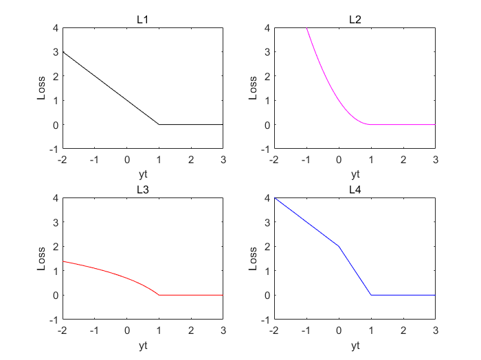
Refer to caption
Figure 2: The support vector loss function L1L_{1}, L2L_{2}, L3L_{3} and L4L_{4}. All are shown as a function of y​tyt rather than tt, because of the symmetry between the y=+1y=+1 and y=−1y=-1 case.

Let K1K_{1} be the Gaussian kernel, that is,

K1(𝒙,𝒙′)=exp(−σ2∥𝒙−𝒙′∥2)=∑𝒏∈(ℕ0)dϕ𝒏(𝒙)ϕ𝒏(𝒙′),σ>0,∀𝒙,𝒙′∈X,K_{1}(\boldsymbol{x},\boldsymbol{x}^{\prime})=\exp(-\sigma^{2}\|\boldsymbol{x}-\boldsymbol{x}^{\prime}\|^{2})=\sum_{\boldsymbol{n}\in(\mathbb{N}_{0})^{d}}\phi_{\boldsymbol{n}}(\boldsymbol{x})\phi_{\boldsymbol{n}}(\boldsymbol{x}^{\prime}),\ \sigma>0,\ \forall\boldsymbol{x},\boldsymbol{x}^{\prime}\in X,

where ϕ𝒏​(𝒙)=∏j=1d(2njnj!)12​(σ​xj)nj​exp−σ2​(xj)2,∀𝒙=(x1,x2,…,xd)T∈X\phi_{\boldsymbol{n}}(\boldsymbol{x})=\prod_{j=1}^{d}\left(\frac{2^{n_{j}}}{n_{j}!}\right)^{\frac{1}{2}}(\sigma x_{j})^{n_{j}}\exp^{-\sigma^{2}(x_{j})^{2}},\ \forall\boldsymbol{x}=(x_{1},x_{2},...,x_{d})^{T}\in X. Also, let K2K_{2} be the min kernel, that is, for any 𝒙,𝒙′∈X\boldsymbol{x},\boldsymbol{x}^{\prime}\in X,

K2​(𝒙,𝒙′)=∏j=1d(min⁡{xj,xj′}−xj​xj′)=∑𝒏∈ℕdϕ𝒏​(𝒙)​ϕ𝒏​(𝒙′),K_{2}(\boldsymbol{x},\boldsymbol{x}^{\prime})=\prod_{j=1}^{d}\left(\min\{x_{j},x_{j}^{\prime}\}-x_{j}x_{j}^{\prime}\right)=\sum_{\boldsymbol{n}\in\mathbb{N}^{d}}\phi_{\boldsymbol{n}}(\boldsymbol{x})\phi_{\boldsymbol{n}}(\boldsymbol{x}^{\prime}),

where ϕ𝒏​(𝒙)=∏j=1d2nj​π​sin⁡(nj​π​xj),∀𝒙=(x1,x2,…,xd)T∈X\phi_{\boldsymbol{n}}(\boldsymbol{x})=\prod_{j=1}^{d}\frac{\sqrt{2}}{n_{j}\pi}\sin(n_{j}\pi x_{j}),\ \forall\boldsymbol{x}=(x_{1},x_{2},...,x_{d})^{T}\in X. For any m∈ℕm\in\mathbb{N}, we can construct ℬK12​m2​m−1​(X)\mathcal{B}_{K_{1}}^{\frac{2m}{2m-1}}(X) and ℬK22​m2​m−1​(X)\mathcal{B}_{K_{2}}^{\frac{2m}{2m-1}}(X).

In each experiment, we select the training data, a loss function and a RKBS above and some suitable parameters, and use Algorithm 1 for training. Since {sk}\{s_{k}\} is globally convergent to a stationary point of Optimization (2.1), we solve Optimization (2.1) repeatedly by selecting some initial values randomly and choosing the minimizer of these outputs as the approximate solution sD2​m2​m−1:X→ℝs_{D}^{\frac{2m}{2m-1}}:X\to\mathbb{R} to build the SVM

ℛ​sD2​m2​m−1​(𝒙)={+1,sD2​m2​m−1​(𝒙)≥0,−1,sD2​m2​m−1​(𝒙)<0.\mathcal{R}s_{D}^{\frac{2m}{2m-1}}(\boldsymbol{x})=\begin{cases}+1,&s_{D}^{\frac{2m}{2m-1}}(\boldsymbol{x})\geq 0,\\ -1,&s_{D}^{\frac{2m}{2m-1}}(\boldsymbol{x})<0.\end{cases}

to make the prediction on testing data. Recall that 𝒜K2​m\mathcal{A}_{K}^{2m} is the sum of infinite terms and is absolutely uniformly convergent, we truncate 𝒜K2​m\mathcal{A}_{K}^{2m} by MM terms and use (𝒜K2​m)M(\mathcal{A}_{K}^{2m})_{M} instead of 𝒜K2​m\mathcal{A}_{K}^{2m} to deal with the infinite sum and reduce the computation, that is,

𝒜K2​m≈(𝒜K2​m)M=∑n∈ℕM(𝚽n)⊗2​m.\mathcal{A}_{K}^{2m}\approx(\mathcal{A}_{K}^{2m})_{M}=\sum\limits_{n\in\mathbb{N}_{M}}(\boldsymbol{\Phi}_{n})^{\otimes 2m}.

It is clear that limM→∞(𝒜K2​m)M=𝒜K2​m\lim\limits_{M\to\infty}(\mathcal{A}_{K}^{2m})_{M}=\mathcal{A}_{K}^{2m}. If M≥N⁡(N+1)/2M\geq N(N+1)/2 and (𝒜K2​m)M(\mathcal{A}_{K}^{2m})_{M} satisfies Assumption 4.1 (iv), then we make sure the convergence of Algorithm 1 with the loss functions and kernels above. Next, we discuss how to solve Optimization (S-1’) by breaking them in NN Optimizations in ℝ\mathbb{R}. To illustrate above, we give a simple example. For the loss function L1L_{1}, by simple algebra, we have that if yi=+1y_{i}=+1, then

(𝜶k+1)i={ei+1β​Nei<1−1β​N,11−1β​N≤ei<1,eiei≥1,​i=1,2,…,N,(\boldsymbol{\alpha}_{k+1})_{i}=\begin{cases}e_{i}+\frac{1}{\beta N}&e_{i}<1-\frac{1}{\beta N},\\ 1&1-\frac{1}{\beta N}\leq e_{i}<1,\\ e_{i}&e_{i}\geq 1,\end{cases}\ \ i=1,2,...,N,

where ei=(𝒜K2​m​(𝒄k)2​m−1)i−1β​(𝜸k)ie_{i}=(\mathcal{A}_{K}^{2m}(\boldsymbol{c}_{k})^{2m-1})_{i}-\frac{1}{\beta}(\boldsymbol{\gamma}_{k})_{i}. On the other hand, if yi=−1y_{i}=-1, then

(𝜶k+1)i={eiei<−1,−1−1≤ei<−1+1β​N,ei−1β​Nei≥−1+1β​N.(\boldsymbol{\alpha}_{k+1})_{i}=\begin{cases}e_{i}&e_{i}<-1,\\ -1&-1\leq e_{i}<-1+\frac{1}{\beta N},\\ e_{i}-\frac{1}{\beta N}&e_{i}\geq-1+\frac{1}{\beta N}.\end{cases}

Next we introduce our test results on synthetic data and real data.

5.1 Examples on Synthetic Data

In this subsection, we introduce our test results on the synthetic data. First, we use a training set D11D_{11} with 25 points and a testing set D12D_{12} with 2601 points to show the effectiveness of Algorithm 1.

Refer to caption
(a) Training Set D11D_{11}
Refer to caption
(b) Testing Set D12D_{12}
Figure 3: The binary classification X1=[−1,1]×[−1,1]X_{1}=[-1,1]\times[-1,1] and Y={+1,−1}Y=\{+1,-1\}: The classes are coded as a binary variable (blue=+1+1 and red=−1-1). The left panel represents the training data D11D_{11} and the right panel represents the testing data D12D_{12}.

First, we show the convergence of Algorithm 1. The selection of relevant parameters in this numerical experiments is given below which satisfies Assumption 4.1.

  • •

    Gaussian kernel K1K_{1}, where σ=1\sigma=1.

  • •

    The loss functions L1L_{1}, L2L_{2}, L3L_{3} and L4L_{4}.

  • •

    The RKBS ℬK12​(X1)\mathcal{B}_{K_{1}}^{2}(X_{1}), ℬK143​(X1)\mathcal{B}_{K_{1}}^{\frac{4}{3}}(X_{1}) and ℬK165​(X1)\mathcal{B}_{K_{1}}^{\frac{6}{5}}(X_{1}).

  • •

    N=25N=25, λ=0.04\lambda=0.04, β=0.1\beta=0.1, μ=10−6\mu=10^{-6} and ε0=10−12\varepsilon_{0}=10^{-12}.

  • •

    we choose 20 initial values randomly in [−1,1]N[-1,1]^{N}.

By Theorem 4.1, we can show the convergence of the sequence {sk}\{s_{k}\} by

∑k∈ℕ‖Ψ⁡(sk+1)−Ψ⁡(sk)‖ℬK12​m​(X1)=∑k∈ℕ(∑n∈ℕ|𝚽nT​(𝒄k+1−𝒄k)|2​m)12​m.\sum\limits_{k\in\mathbb{N}}\|\Psi(s_{k+1})-\Psi(s_{k})\|_{\mathcal{B}_{K_{1}}^{2m}(X_{1})}=\sum_{k\in\mathbb{N}}\left(\sum_{n\in\mathbb{N}}\left|\boldsymbol{\Phi}_{n}^{T}(\boldsymbol{c}_{k+1}-\boldsymbol{c}_{k})\right|^{2m}\right)^{\frac{1}{2m}}.

We use (𝒜K2​m)M(\mathcal{A}_{K}^{2m})_{M} instead of 𝒜K2​m\mathcal{A}_{K}^{2m} and we have that

∑k∈ℕ‖Ψ⁡(sk+1)−Ψ⁡(sk)‖ℬK12​m​(X1)≈∑k∈ℕ(∑n∈ℕM|𝚽nT​(𝒄k+1−𝒄k)|2​m)12​m.\sum_{k\in\mathbb{N}}\|\Psi(s_{k+1})-\Psi(s_{k})\|_{\mathcal{B}_{K_{1}}^{2m}(X_{1})}\approx\sum_{k\in\mathbb{N}}\left(\sum_{n\in\mathbb{N}_{M}}\left|\boldsymbol{\Phi}_{n}^{T}(\boldsymbol{c}_{k+1}-\boldsymbol{c}_{k})\right|^{2m}\right)^{\frac{1}{2m}}.

We now conduct experiments to verify convergence of Algorithm 1 with nonconvex loss function L3L_{3}.

Refer to caption
(a) m=1m=1
Refer to caption
(b) m=2m=2
Refer to caption
(c) m=3m=3
Figure 4: The convergence of Algorithm 1 in different RKBSs with the loss function L3L_{3}. The horizontal axis represents iterations and the vertical axis represents ∑k∈ℕ‖Ψ⁡(sk+1)−Ψ⁡(sk)‖ℬK12​m​(X1)\sum\limits_{k\in\mathbb{N}}\|\Psi(s_{k+1})-\Psi(s_{k})\|_{\mathcal{B}_{K_{1}}^{2m}(X_{1})}.

As shown in Figure 4, for the training data D11D_{11}, loss function L3L_{3} and other parameters above, Algorithm 1 converges in less than 50 iterations. These numerical results shows that Algorithm 1 is efficient and stable. Next, we use other loss functions mentioned above to test Algorithm 1 and reveal the advantage of the SVM in general RKBS with nonconvex loss function through comparing the performance in different RKBSs with different lower semi-continuous loss functions. Here are the results of these experiments:

Table 1: Different Testing Accuracy on Testing Set D12D_{12}.
RKBSLoss L1L_{1} L2L_{2} L3L_{3} L4L_{4}
ℬK12​(X1)\mathcal{B}_{K_{1}}^{2}(X_{1}) 90.3% 92.0% 89.1% 91.4%
ℬK143​(X1)\mathcal{B}_{K_{1}}^{\frac{4}{3}}(X_{1}) 90.3% 91.4% 91.2% 92.5%
ℬK165​(X1)\mathcal{B}_{K_{1}}^{\frac{6}{5}}(X_{1}) 91.2% 91.4% 85.2% 93.2%

From Table 1, it shows that the SVM in RKBS with lower semi-continuous loss function by Algorithm 1 is feasible in terms of accuracy. Moreover, it is easy to see that for this training data D11D_{11} and testing data D12D_{12}, the SVM in ℬK165​(X1)\mathcal{B}_{K_{1}}^{\frac{6}{5}}(X_{1}) with the nonconvex loss function L4L_{4} performs better than other case shown in Table 1. However, when mm is larger, the performance of corresponding SVM is not necessarily better, such as the performance of L3L_{3} above. Next, we introduce the numerical experiment result on another dataset.

We sample from Ω1=[0.4,1]×[0.4,1]\Omega_{1}=[0.4,1]\times[0.4,1] labeled by +1+1 and Ω2=[0,0.6]×[0,0.6]\Omega_{2}=[0,0.6]\times[0,0.6] labeled by −1-1 randomly to obtain training set D21D_{21} and testing set D22D_{22}. The data labeled by +1+1 are equal to the data labeled by −1-1 in D21D_{21} or D22D_{22}. Here is an example of sampling. In the following figures, two subdatasets are colored in blue and red.

Refer to caption
(a) Training Set D21D_{21}
Refer to caption
(b) Testing Set D22D_{22}
Figure 5: An example of sampling where X2=[0,1]×[0,1]X_{2}=[0,1]\times[0,1] and Y={+1,−1}Y=\{+1,-1\}. The classes are coded as a binary variable (blue=+1+1 and red=−1-1). The left panel represents the training data D21D_{21} and the right panel represents the testing data D22D_{22}.

Next, we use a training set D21D_{21} with 300 points and a testing set D22D_{22} with 120 points to show the effectiveness of Algorithm 1. Here are some parameters and results of these experiments:
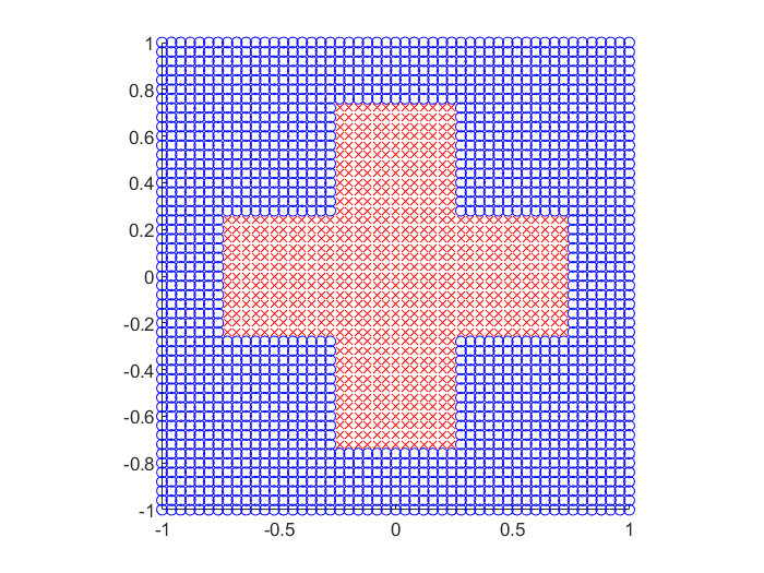
  • •

    Min kernel K2K_{2}.

  • •

    The loss functions L1L_{1}, L2L_{2}, L3L_{3} and L4L_{4}.

  • •

    The RKBS ℬK22​(X2)\mathcal{B}_{K_{2}}^{2}(X_{2}), ℬK243​(X2)\mathcal{B}_{K_{2}}^{\frac{4}{3}}(X_{2}) and ℬK265​(X2)\mathcal{B}_{K_{2}}^{\frac{6}{5}}(X_{2}).

  • •

    N=300N=300, λ=0.01\lambda=0.01, β=1\beta=1 and ε0=10−12\varepsilon_{0}=10^{-12}.

  • •

    Choose 2020 initial values randomly in [0,1]N[0,1]^{N}.

Table 2: Different Testing Accuracy on Testing Set D22D_{22}.
RKBSLoss L1L_{1} L2L_{2} L3L_{3} L4L_{4}
ℬK22​(X2)\mathcal{B}_{K_{2}}^{2}(X_{2}) 90.0% 90.0% 90.0% 89.2%
ℬK243​(X2)\mathcal{B}_{K_{2}}^{\frac{4}{3}}(X_{2}) 89.2% 90.0% 89.2% 90.8%
ℬK265​(X2)\mathcal{B}_{K_{2}}^{\frac{6}{5}}(X_{2}) 90.0% 90.0% 89.2% 90.0%

From Table 2, we check that the SVM in ℬK243​(X2)\mathcal{B}_{K_{2}}^{\frac{4}{3}}(X_{2}) with nonconvex loss function L4L_{4} performs better than others. It shows that in some cases the SVM in RKBS is more suitable than the classical SVM in RKHS. Next we introduce our experiments on real data.

5.2 Examples on UCI Machine Learning Repository

We choose the banknote authentication dataset in UCI Machine Learning Repository to test Algorithm 1. The data were extracted from images that were taken from genuine and forged banknote-like specimens. Wavelet Transform tool were used to extract features from images. There are 4 input variables about them, which are variance, skewness, curtosis of wavelet transformed image and entropy of image. Using principal component analysis, we select 33 main input variables (variance, skewness, curtosis of wavelet transformed image) and denote the sample space X3=[−20,20]3X_{3}=[-20,20]^{3} and the label space Y={+1,−1}Y=\{+1,-1\}. Next, we choose 200200 images randomly as training set D31D_{31}, and a half of them are labeled by +1+1 and the others are labeled by −1-1. Also, we choose 100100 images randomly as testing set D32D_{32}, and a half of them are labeled by +1+1 and the others are labeled by −1-1. We introduce some parameters of these experiments:

  • •

    The kernels K1K_{1}, where σ=0.5\sigma=0.5.

  • •

    The loss functions L1L_{1}, L2L_{2}, L3L_{3} and L4L_{4}.

  • •

    The RKBS ℬK12​(X3)\mathcal{B}_{K_{1}}^{2}(X_{3}), ℬK143​(X3)\mathcal{B}_{K_{1}}^{\frac{4}{3}}(X_{3}) and ℬK165​(X3)\mathcal{B}_{K_{1}}^{\frac{6}{5}}(X_{3}).

  • •

    N=200N=200, λ=0.01\lambda=0.01, β=0.01\beta=0.01 and ε0=10−12\varepsilon_{0}=10^{-12}.

  • •

    Choose 2020 initial values randomly in [−1,1]N[-1,1]^{N}.

In each experiment, we will choose a loss function and an RKBS. Then we have the following results.

Table 3: Different Testing Accuracy of on Testing Set D32D_{32}.
RKBSLoss L1L_{1} L2L_{2} L3L_{3} L4L_{4}
ℬK12​(X3)\mathcal{B}_{K_{1}}^{2}(X_{3}) 87.0% 85.0% 86.0% 79.0%
ℬK143​(X3)\mathcal{B}_{K_{1}}^{\frac{4}{3}}(X_{3}) 86.0% 82.0% 88.0% 86.0%
ℬK143​(X3)\mathcal{B}_{K_{1}}^{\frac{4}{3}}(X_{3}) 86.0% 82.0% 86.0% 86.0%

From Table 3, we check that the SVM in ℬK143​(X3)\mathcal{B}_{K_{1}}^{\frac{4}{3}}(X_{3}) with nonconvex loss function L3L_{3} performs better than others in these experiments. It shows that in some cases the nonconvex loss function and RKBS are more suitable than the convex loss function and RKHS, which is our motivation of this paper.

In Section 5, we demonstrate the effectiveness of solving the SVM in RKBS with lower semi-continuous loss function by splitting method based on ADMM. In addition, we give some examples to show that in some cases, the SVM in RKBS with lower semi-continuous loss function is better than the SVM in RKHS with convex loss function. Therefore, we can consider not only RKHS and convex loss function, but also RKBS and nonconvex loss function.

6 Final Remarks

In the paper [15], the second author and the third author propose several numerical tricks in RKBS and discuss the homotopy method for the multikernel-based approximation method. As a continuation of the program, in this paper, we discuss the splitting method based on ADMM for the SVM in ℬK2​m2​m−1​(X)\mathcal{B}_{K}^{\frac{2m}{2m-1}}(X) with lower semi-continuous loss function. Since ℬKp​(X)​(1≤p<∞)\mathcal{B}_{K}^{p}(X)\ (1\leq p<\infty) are also RKBSs, from [29, Chapter 5] and [13, Corollary 4.1], the SVM in ℬKp​(X)​(1≤p<∞)\mathcal{B}_{K}^{p}(X)\ (1\leq p<\infty) have a minimizer. Since ℬKp​(X)​(p>1)\mathcal{B}_{K}^{p}(X)\ (p>1) has similar property with ℬK2​m2​m−1​(X)\mathcal{B}_{K}^{\frac{2m}{2m-1}}(X), we try to use similar line of arguments therein to deal with. Although ℬK1​(X)\mathcal{B}_{K}^{1}(X) is not reflexive, strictly convex or smooth, we can use the SVM in ℬKp​(X)​(1<p<∞)\mathcal{B}_{K}^{p}(X)\ (1<p<\infty) to approximate the SVM in ℬK1​(X)\mathcal{B}_{K}^{1}(X). Next we will study how to solve the SVM in ℬKp​(X)​(1≤p<∞)\mathcal{B}_{K}^{p}(X)\ (1\leq p<\infty) with lower semi-continuous loss function.

References

  • [1] A. Beck. First-Order Methods in Optimization. SIAM, Philadelphia, 2017.
  • [2] D. Bertsekas. Convex Optimization Theory. Athena Scientific, Nashua, NH, 2009.
  • [3] J. Bolte, A. Daniilidis and A. Lewis. The Lojasiewicz inequality for nonsmooth subanalytic functions with applications to subgradient dynamical systems. SIAM J. Optimiz., 17 (2007), pp. 1205-1223.
  • [4] J. Bolte, A. Daniilidis, A. Lewis and M. Shiota. Clarke subgradients of stratifiable functions. SIAM J. Optimiz., 18 (2007), pp. 556-572.
  • [5] J. Bolte, S. Sabach and M. Teboulle. Proximal alternating linearized minimization for nonconvex and nonsmooth problems. Math. Program., 146 (2014), pp. 459-494.
  • [6] S. Boyd, N. Parikh, E. Chu, B. Peleato, J. Eckstein, et al. Distributed optimization and statistical learning via the alternating direction method of multipliers. Found. Trends. Mach. Le., 3 (2011), pp. 1-122.
  • [7] J. Brooks. Support Vector Machines with Ramp Loss and the Hard Margin Loss. Oper. Res., 59 (2011), pp. 467-479.
  • [8] C. Cortes and V. Vapnik. Support Vector Network. Mach. Learn., 20 (1995), pp. 273-297.
  • [9] H. Dales, F. Dashiell, A. Tau and D. Strauss. Banach Spaces of Continuous Functions as Dual Spaces. Springer, Switzerland, 2016.
  • [10] F. Facchinei and J. Pang. Finite-Dimensional Variational Inequalities and Complementarity Problems, vol.I. Springer, Berlin, 2003.
  • [11] Y. Feng, Y. Yang, S. Huang, S. Mehrkanoon and J. Suykens. Robust Support Vector Machines for Classification with Nonconvex and Smooth Losses. Neural Comput., 28 (2016), pp. 1217-1247.
  • [12] K. Guo, D. Han and T. Wu. Convergence of alternating direction method for minimizing sum of two nonconvex functions with linear constraints. Int. J. Comput. Math., 94 (2016), pp. 1-18.
  • [13] L. Huang, C. Liu, L. Tan and Q. Ye. Generalized representer theorems in Banach spaces. Anal. Appl., 19 (2021), pp. 125-146.
  • [14] G. Li and T. Pong. Global convergence of splitting methods for nonconvex composite optimization. SIAM J. Optimiz., 25 (2015), pp. 2434-2460.
  • [15] Y. Lin, Y. Wei and Q. Ye. A Homotopy Method for Multikernel-based Approximation. J. Nonlinear Var. Anal., 6 (2022), pp. 139-154.
  • [16] D. Liu, Y. Shi, Y. Tian and X. Huang. Ramp loss least squares support vector machine. J. Comput. Sci-Neth., 14 (2016), pp. 61-68.
  • [17] R. Megginson. An Introduction to Banach Space Theory. Springer-Verlag, New York, 1998.
  • [18] M. Mo and Q. Ye. Splitting Method for Support Vector Machines with Lower Semi-continuous Loss. arXiv preprint, arXiv:2208.12522, 2022.
  • [19] B. Mordukhovich. Variational Analysis and Generalized Differentiation. I: Basic Theory. Grundlehren Series (Fundamental Principles of Mathematical Sciences), Springer, Berlin, 2006.
  • [20] J. Ortega and W. Rheinboldt. Iterative Solution of Nonlinear Equations in Several Variables. Academic Press, inc, San Diego, 1970.
  • [21] L. Qi, H. Chen and Y. Chen. Tensor Eigenvalues and Their Applications. Springer, Singapore, 2018
  • [22] R. Rockafellar and R. Wets. Variational Analysis. Springer Berlin Heidelberg, Berlin, 1998.
  • [23] W. Rudin. Principles of mathematical analysis. McGraw-Hill, Inc, New York, 1976.
  • [24] X. Shen, L. Niu, Z. Qi. and Y. Tian, Support Vector Machine Classifier with Truncated Pinball Loss. Pattern Recogn., 68 (2017), pp. 199-210.
  • [25] M. Shiota. Geometry of Subanalytic and Semialgebraic Sets. Birkhäuser, Boston, 1998.
  • [26] I. Steinwart and A. Christmann. Support Vector Machines. Springer-Verlag, New York, 2008.
  • [27] M. Unser. A Unifying Representer Theorem for Inverse Problems and Machine Learning. Found. Comput. Math., 21 (2021), pp. 941–960.
  • [28] H. Wang, Y. Shao, S. Zhou, C. Zhang and N. Xiu. Support vector machine classifier via L0/1 soft-margin loss. IEEE T. Pattern Anal., 44 (2022), pp. 7253-7265.
  • [29] Y. Xu and Q. Ye. Generalized Mercer kernels and reproducing kernel Banach spaces. Mem. Am. Math. Soc., 258 (2019), pp. 1-122.
  • [30] Y. Xu and W. Yin. A block coordinate descent method for regularized multiconvex optimization with applications to nonnegative tensor factorization and completion. SIAM J. Imaging Sci., 6 (2013), pp. 1758–1789.
  • [31] Q. Ye. Positive Definite Multi-kernels for Scattered Data Interpolations. Appl. Comput. Harmon. A., 62 (2023), pp. 251-260.


Mingyu Mo

School of Mathematical Sciences

South China Normal University

Guangzhou, 510631, Guangdong, PR China

Email-address: mmymaths@qq.com.

Yimin Wei

School of Mathematical Sciences

Fudan University

Shanghai, PR China

Email-address: ymwei@fudan.edu.cn.

Qi Ye

School of Mathematical Sciences

South China Normal University

Guangzhou, 510631, Guangdong, PR China

Pazhou Lab

Guangzhou, 511442, Guangdong, PR China.

Email-address: yeqi@m.scnu.edu.cn.