Snapshot disjointness in temporal graphs
Abstract
In the study of temporal graphs, only paths respecting the flow of time are relevant. In this context, many concepts of walks disjointness were proposed over the years, and the validity of Menger’s Theorem, as well as the complexity of related problems, has been investigated. In this paper, we introduce and investigate a type of disjointness that is only time dependent. Two walks are said to be snapshot disjoint if they are not active in a same snapshot (also called timestep). The related paths and cut problems are then defined and proved to be -hard and -time solvable when parameterized by the size of the solution. Additionally, in the light of the definition of Mengerian graphs given by Kempe, Kleinberg and Kumar in their seminal paper (STOC’2000), we define a Mengerian graph for time as a graph that cannot form an example where Menger’s Theorem does not hold in the context of snapshot disjointness. We then give a characterization in terms of forbidden structures and provide a polynomial-time recognition algorithm. Finally, we also prove that, given a temporal graph and a pair of vertices , deciding whether at most multiedges can separate from is -complete.
1 Introduction
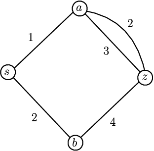
A temporal graph can be described as a graph that varies in time. Such objects can be modeled in different ways, usually according to the application being considered, and have appeared in the literature under many names as for instance dynamic networks [19], temporal networks [9], time-varying graphs [4], etc. For surveys we refer the reader to [9, 14]. In this paper, we consider a temporal graph to be a pair , where is a multigraph (hereon called just graph) and is a function, called timefunction, that relates each edge to a discrete label telling when such edge is going to be active. The value is called lifetime and is denoted by . Also, graph is called the base graph. See Figure 1a for an example.


Many practical problems are modeled in temporal graphs (see [9] for a nice collection of practical examples), and among the most common ones are those related to temporal walks and connectivity. A temporal walk is a walk that respects the flow of time; for simplicity, we represent them as sequences of vertices and timesteps. For instance, in Figure 1a, the sequence is a temporal walk between and (also called temporal -walk). A temporal path is then defined as a temporal walk whose internal vertices are all distinct. Hence, the previously mentioned temporal -walk is not a path, while the walk is a temporal path. Additionally, some authors deal only with walks and paths whose edges are active in strictly increasing times; in such case, is a valid temporal -path, while is not. To distinguish from these, we say that a walk/path is strict if the edges are active in strictly increasing times, and that it is non-strict if they are active in non-decreasing times.
In contrast with classic graph theory, when dealing with walks and paths in temporal graphs, it is not always the case that the problems defined on walks are equivalent to those defined on paths. See for instance [1, 5, 7, 10]. This is not the case for the problems investigated here, and this is why we interchangeably use the terms walks and paths.
Connectivity problems concern the robustness of a network, which translates into knowing how many independent (or disjoint) ways there are to go from one vertex to another, and how easy it is to break such connections. In this paper, we introduce a new robustness concept that relies on the time aspect of a network. To better understand these concepts, consider the following scenario. Suppose a temporal graph models a communication network. Such network might be prone to interruptions of all communications at a given timestep due to attacks, blackouts, maintenance, etc. A good measure of robustness of such networks could then be the minimum number of timesteps in which the communications must get interrupted in order to break all possible connections between a pair of vertices. A network with higher measure means that it is less susceptible to failing under such interruptions and hence is considered more robust. In Figure 1a, for instance, if there is an interruption on timesteps and , then vertex cannot relay a message to anymore, while it still can relay messages to through the path .
To model such scenario, we say that two temporal -paths and are snapshot disjoint if, at any given timestep, at most one between and is traversing any edges. For example, in Figure 1a, paths and are two snapshot disjoint temporal -paths. We also say that a set of timesteps is a snapshot -cut if every temporal -path uses an edge active in timestep for some . For example, in Figure 1a, is a snapshot -cut. The following problems are then defined.
-snapshot -cut
Input. A temporal graph , vertices , and an integer .
Question. Is there a snapshot -cut in of size at most ?
-snapshot disjoint temporal -paths
Input. A temporal graph , a pair of vertices , and a positive integer .
Question. Is there a set of snapshot disjoint temporal -paths in of size at least ?
We prove that, when parameterized by and respectively, both problems are -hard, and that this is best possible, i.e., that they are also . While the algorithm for snapshot -cut follows easily from the definition and the fact that we can test all possible cuts in time (namely, time), the algorithm for snapshot disjoint temporal -paths is much more involved and uses a technique similar to the one applied to find vertex disjoint paths between given pairs of vertices (also known as the -linkage problem) in a DAG [17]. As we will see in the related works, this is the first result of such kind, with all previously defined disjointness either having the related paths problem polynomial-time solvable or para--complete (i.e., -complete for fixed values of ).
A celebrated result in classic graph theory tells us that, in a graph and for every pair , the maximum number of internally vertex disjoint -paths is equal to the minimum size of an -cut (vertices whose removal breaks all -paths). This is the well known Menger’s Theorem, and it holds on both undirected and directed graphs, as well as for edge-disjoint paths and edge cuts. When translating these concepts to temporal graphs, it is natural to ask whether a version of Menger’s Theorem holds. The answer in our context is no, as can be witnessed by the example in Figure 1b. Note that any two temporal -paths intersect in some timestep, while there is no snapshot -cut of size 1. Indeed, does not use edges active in timestep , does not use 1, and does not use 2.
In their seminal paper, Kempe, Kleinberg and Kumar [13], in the context of vertex disjoint temporal paths, defined a Mengerian graph as being a graph where Menger’s Theorem would hold for whatever choice of timefunction. They then characterize these graphs when constrained to simple graphs (every multiedge has multiplicity 1), and more recently their result was generalized to allow for multigraphs [11]. Here, we say that is Mengerian for time if, for every timefunction and every , the maximum number of snapshot disjoint temporal -paths in is equal to the minimum size of a snapshot -cut. In other words, the snapshot disjoint version of Menger’s Theorem always holds on temporal graphs whose base graph is . We then give the following characterization. The formal definition of an m-topological minor is given in Section 2, but for now it suffices to say that, when subdividing an edge , the multiplicity of the obtained edges is the same as .

Theorem 1.
Let be a graph. Then is Mengerian for time if and only if does not have any of the graphs in Figure 2 as m-topological minor. Moreover, we can recognize whether is Mengerian for time in polynomial time.
Finally, in order to fill an open entry related to multiedge disjoint temporal paths (the definition is presented shortly), we prove in Section 6 that the related cut problem is -complete even if the temporal graph has lifetime equal to 2.
Related problems.
As snapshot disjointness is a newly introduced concept, no previous results exist. We then refer the reader to the many results about Menger’s related concepts in temporal graphs. In this context, the vertex disjoint version of Menger’s Theorem was proved not to hold by Berman [3]. Since then a number of papers have investigated the complexity of related problems [13, 20], as well as new structural concepts like the definition of Mengerian graphs [13, 11], and adaptations to temporal vertex disjoint versions [16, 10]. Because our problem is more closely related to edge connectivity, we refrain from commenting in details the results on vertex connectivity, but refer the reader to [10] for an overview of such results. In what follows, we present the edge-related concepts and existing results. These are summarized in Table 1.
| Non-strict | Strict | |||
|---|---|---|---|---|
| -Walks | -Cut | -Walks | -Cut | |
| Multiedge | c [3], if dir., | c for | c for [12] | c for [2] |
| even for | (Theorem 11) | and [15] | and for [8] | |
| Edge | Polynomial [3] | Polynomial [16] | ||
| Snapshot | for (Th. 6) | for (Th. 7) | Open | |
| for (Th. 5) | for (Th. 4) | |||
| Node dep. | Open | Polynomial [16] | ||
A set of temporal -walks are edge disjoint if they share no edges, and are multiedge disjoint if they share no multiedges. For example, in Figure 1a, the paths and are edge disjoint, but are not multiedge disjoint, since they share the multiedge with endpoints . A set of (multi)edges is a temporal (multi)edge -cut if they intersect every temporal -walk. For example, in Figure 1a, and form a multiedge -cut, but if we want an edge -cut, we have to pick both edges whose endpoints are . In some works, instead of using a multigraph, it is used a simple graph together with a timefunction that assigns to each edge a finite set of positive integers. In such cases, an edge in our context would be called a temporal edge, while a multiedge in our context would be a simple edge of the base graph.
In [3], Berman showed that the edge problems for non-strict temporal paths are polynomial-time solvable, and that deciding the existence of at least multiedge disjoint temporal paths is -complete, directed or undirected, and if is directed, then the same holds even if . Up to our knowledge, no result concerning the cut problem related to multiedges was presented so far. By a simple modification of a proof in [20], we present in Section 6 a proof of -completeness of the multiedge cut problem. Our proof works also for the case where is a directed multigraph. Concerning strict paths, the complexities of these problems follow directly from results about problems on bounded length paths [2, 8]. Additionally, the strict problems related to edge disjoint paths was shown to be polynomial-time solvable in [16]. We mention that, among all the problems appearing in Table 1, Menger’s Theorem holds only for edge disjoint paths in both the strict and non-strict contexts [3, 16], and node departure disjoint strict paths, defined below.
Another related concept is that of node departure disjoint, introduced in [16]. Given a temporal graph with lifetime , a set of strict temporal -walks is node departure disjoint if no two of these paths leave a vertex in the same timestep. For example, in Figure 1a, and are node departure disjoint. Additionally, a set is a node departure -cut if all strict temporal -walks contains an edge departing from in time , for some . For example, in Figure 1a, the set is a node departure -cut. In [16], the authors prove that the maximum number of node departure disjoint -walks is equal to the minimum size of a node departure -cut. Even though the authors do not comment on the complexity of the related problems, their proof leads to a polynomial time algorithm as it consists of building a flow network and proving that the searched values are equivalent to applying the famous Maxflow-Mincut Theorem. Up to our knowledge, their results have not been investigated for the non-strict context.
The text is organized as follows. In Section 2, we present definitions, terminology and some basic results. In Section 3, we present our algorithms. In Section 4, we prove that -snapshot -cut and -snapshot disjoint temporal -paths are [1]-hard when parameterized by and , respectively. In Section 5, we characterize Mengerian graphs. Finally, in Section 6, we prove that -Multiedge cut is -complete, and in Section 7 we present our concluding remarks.
2 Definitions and Terminology
Given positive integers such that , we denote by the set and by the set .
A graph is a triple where and are finite sets that we call vertex set and edge set respectively, and is a function that, for each associates a pair of elements in , where . We say that edge is incident to and , that are the endpoints of , and that connects and . We omit in the rest of the paper and refer simply to the endpoints of instead. We also call the pair a multiedge, and the number of edges with endpoints is the multiplicity of the multiedge . If the multiplicity of each edge is 1, we say that is a simple graph. We denote by the simple graph obtained from by decreasing the multiplicity of all multiedges to 1. See [18] for further basic definitions of graph theory.
Given a graph and a set of vertices , the identification of is the graph obtained from by adding a new vertex and, for every edge with endpoints where and , add an edge with endpoints . The graph obtained from by a subdivision of an edge with endpoints is the graph having as vertex set, and as edge set, where has endpoints and has endpoints . Finally, the graph obtained from by an m-subidivision of a multiedge is the graph obtained by subdividing all the edges with endpoints and then identifying the new vertices. Observe Figure 3 for an illustration of these definitions. The definition of m-subdivision has been introduced in [11]. Given a graph , if has a subgraph that can be obtained from m-subdivisions of , then we say that is an m-topological minor of .

A temporal graph is a pair where is a graph and . Depending on the context we refer to the elements of as timesteps. If an edge is such that we say that is active or appears at timestep . A temporal -walk in is a sequence that alternates vertices and edges such that for every , is an edge between and and . If for every with , we say that such temporal walk is a temporal path. Moreover, we define and . For our purposes, we can assume that the subgraph active at a given timestep is simple, i.e., that if and have both endpoints , then . Such assumption allows us to define a path as a sequence of vertices and timesteps such that, for each , there is an edge connecting active at timestep . The lifetime of is denoted by and is the maximum integer such that there is an edge of active at such timestep. For each timestep , the -th snapshot of is the subgraph of defined as .
Let be a temporal graph with lifetime . Also, let be vertices in and temporal -paths. We say that and are snapshot disjoint if . A subset is a snapshot -cut if every temporal -path uses an edge active at some timestep in . We denote by the maximum number of snapshot disjoint temporal -paths and by the minimum size of a snapshot -cut. Observe that if the above definitions are made in terms of temporal paths, then these parameters would not change. A graph is Mengerian (for time) if, for every timefunction on , and every , , we have that . The following will be useful later, and the proofs can be found in Appendix A.
Proposition 2.
If is non-Mengerian, then an m-subdivision of is also non-Mengerian.
Proposition 3.
is Mengerian if and only if is Mengerian, for every .
3 Positive Results
In this section, we give algorithms for both snapshot -cut and snapshot disjoint temporal -paths. Given the results of Section 4, unless -hard, algorithms are best possible from the point of view of parameterized complexity. The first algorithm is quite simple and consists of the usual approach of testing all possible cuts.
Theorem 4.
Given a temporal graph of lifetime , a positive integer and , we can solve -snapshot -cut in .
The next algorithm is much more involved, and uses a technique similar to the one used to find disjoint paths between given pairs of vertices in a DAG [17].
Theorem 5.
Given a temporal graph , vertices and a positive integer , we can solve snapshot disjoint temporal -paths in time , where .
Proof.
We construct a digraph with vertices and such that and there is an -path in if and only if there are snapshot disjoint temporal -paths in .
The vertex set of digraph is equal to the -tuples formed by edges of , together with vertices and ; formally , where . Vertex is set to be equal to , while vertex is set to be equal to . Each dimension of represents one of the desired disjoint paths, and a set of snapshot disjoint temporal -paths will be represented by an -path in , as previously said. So represents the starting point, and represents the finish point of every temporal -path. Then, when an edge of is traversed by , we want that one of the paths also traverses an edge. Because we want to allow that only one of the paths gets closer to with each step of , there will be an edge from to only if exactly one position of and differ. Not only this, but we want that, at each step of , the path that gets closer to is the one whose last traversed edge occurs the earliest among all the ’s. In the next paragraph, we formally construct digraph .
As previously said, let . Along the construction, we will be referring to Figures 4 and 5. Because we want to avoid simultaneous traversal of paths that intersect in a snapshot, we only consider elements of whose edges of all appear in distinct snapshots. Indeed, if and we allow for instance the existence of vertex such that , then this would mean that the constructed paths and intersect in timestep . Therefore, we define as formalized below. Observe that this implies, in Figure 5, that vertices do not exist in , where denotes the edge with endpoints active in timestep 2.

Now, we define the edge set of . For this, we first construct an auxiliary graph whose vertex set is equal to ; observe Figure 4b to follow the construction. First of all, we want that a traversal of an edge in translates into a valid traversal in . Therefore, for every pair , add to an edge from to only if can be followed by in a temporal -path in . Formally, add in the following cases: for every , and every adjacent to and such that ; for and every incident to ; and for every incident to and .
Finally, as previously said, we want that at each edge traversal of an -path in , the path in that is getting closer to is that one whose last used edge is the earliest among all the other paths. To help with this, we also define to be equal to , and to be equal to , where is equal to the lifetime of . This means intuitively that we give always priority to leave , and that, once we reach in any dimension, then we cannot depart from anymore. So, given a vertex , we add an edge from to if and only if:
- •
differ from in exactly one position, ;
- •
is such that ; and
- •
By letting be the value in the -th position of , we have that is a valid move, i.e., that .
Observe Figure 5. Another way of seeing this construction is by starting with copies of on each row and column of , then removing the vertices that do not belong to , and finally removing from row/column any edge leaving with .

Now, we prove that there are snapshot disjoint temporal -paths in if and only if there is an -path in . In what follows, given a vertex , we denote by the tuple related to . Recall that and . Suppose is a set of snapshot disjoint temporal -paths in . For each , let be the sequence of edges used in in order of traversal and define and . By induction, we define a sequence of vertices of , , that forms an -path for some with the following property:
- (P)
For each dimension and each , the sequence of edges traversed in dimension is a subpath of . Formally, by removing and repetitions of edges from the sequence , we obtain a subsequence of .
First, we define ; clearly property (P) holds as all paths start in . Now suppose that sequence satisfying Property (P) is obtained, . Let be such that . By Property (P), observe that either , or is an edge of , or . If the latter occurs, then we get that is an -path in , since for every , i.e., the only way is minimum is if all other positions are also equal to . So suppose one of the other cases occurs. Note that it means that there is some edge following in , say . By definition of temporal path, ; hence . Define to be equal to except that in position we have instead of , and note that is a path in that satisfies Property (P).
Now suppose the existence of an -path in , . We construct a set of snapshot disjoint temporal -paths in . For this, for each , let be a sequence of edges obtained from dimension , i.e., from by removing occurrences of and , and repetitions of edges. Because each transition respects , we trivially get that defines a temporal -path in . It remains to show that such paths are snapshot disjoint. Suppose otherwise, and let be such that there are edges in and in such that . Let be the smallest index such that , and be the smallest index such that . By the definition of , we have that . Indeed no vertex of can contain two elements of with same value of , and recall that as are distinct paths. So, we can suppose, without loss of generality, that . Observe that this means that differ from in exactly position ; additionally, it means that . In particular, we have that . But observe that, in a fixed dimension, the values of can only increase, i.e., since , we get . We get a contradiction as in this case vertex should not be defined as it contains two elements with the same value of , namely and .
To finish the proof just recall that , where , and that deciding if there is a path between two vertices in can be made in time . So, deciding if there are snapshot disjoint temporal -paths in can be done in time . ∎
4 Negative Results
In this section, we prove that the algorithms presented in Section 3 are best possible, i.e., that -snapshot disjoint temporal -paths and -snapshot -cut are [1]-hard when parameterized by and , respectively.
Theorem 6.
-snapshot disjoint temporal -paths is -hard when parameterized by .
Proof.
We make a parameterized reduction from -Independent set when parameterized by . The input of such problem is a simple graph and an integer , and the question is whether has an independent set of size at least . This is known to be -hard (see e.g. [6]).
So consider an instance of -Independent Set and let . Observe Figure 6 to follow the construction. First, add to vertices and . Then, for each , add to an -path on edges; denote such path by . Now, consider any ordering of , and denote the edges incident to a vertex by . We can define in a way that each is a temporal -path using the orders of the edges in . Formally, for each , let with , and define to be equal to in a way that is a temporal path.

Because of space constraints, the proof of correctedness is presented in Appendix C. ∎
Now, we prove the analogous result for the cut problem.
Theorem 7.
-snapshot -cut is -hard when parameterized by .
Proof.
We make a reduction from Multicolored -Clique, when parameterized by , known to be -hard [6]. Such problem has as input a simple graph , an integer , and a partition of into independent sets (alternatively, a proper -coloring), and the question is whether has a (multicolored) clique of size . So let be a graph and be a proper -coloring of . By adding artificial vertices and edges if necessary, we can suppose that the number of edges between and is equal to a value , for every pair . So, for , , denote the set of such edges by . We make this assumption in order to make presentation simpler.
Now, for each , , we construct a gadget denoted by . Observe Figure 7 to follow the construction. First add to the set of vertices , making the first of them form a path of multiplicity , and the latter form a path of multiplicity 1. Formally, for each , add edges with endpoints . Also, for each , add 1 edge with endpoints . Now, for each , add vertex and join such vertex with by a path with edges and denote such path by . We say that vertex of our gadget is associated with edge of . The timefunction is defined only later.

Now, we finish the construction of our temporal graph. For this, take the union of all graphs and identify all vertices , calling the obtained vertex , and identify all vertices , calling the obtained vertex . Also, for each , , and , we add two edges between and . Denote by the obtained graph, and by the set . Observe that contains vertices and edges.
Now we define . The idea is that each will be active during its own dedicated time window. Formally, define , for each pair , , in a way that whenever . Now, consider with . For each , we define in a way that every value in appears in some edge with endpoints . Also, for each , we let , and we define to be equal to and in a way that is a temporal -path. Finally, the only edges that remain unlabelled are the edges between and vertices of type . For such edges, we reserve a time window of size , that we denote by , where any timestep in such set is greater that any timestep we used to define so far. Moreover, we associate each vertex with a timestep . Let and recall that such vertex is associated with . Suppose have endpoints , and let the two edges of with endpoints be active in timesteps .
Now, we prove that has a clique of size if and only if has a snapshot -cut of size at most . Consider first a clique of of size , and let be the set of edges of between vertices of . Notice that, because has a vertex from each part, we get that . Define . We prove that is a snapshot -cut. By contradiction, suppose that is a temporal -path not passing by , i.e., such that . Since and all edges incident to are active in timesteps , we can define to be the index related to the first edge in , i.e., starts in an edge of , say the one active in timestep . Observe that the value is within the temporal -path contained in , and that it also separates and for every . Hence, must start with the temporal -path contained in . However, as is incident to vertices of the clique, say and , then we have that uses timestep or , a contradiction as .
Now, suppose that is a minimum snapshot -cut in and that it has size at most . Let . We prove that is a clique of of size . Denote by the set of pairs . We say that is open if for some , and we say that is the open edge of . The following simple facts will be useful:
- 1.
For every , , we have : this is due to the fact that there is a temporal -path using only timesteps in ;
- 2.
If is such that , then , where are the endpoints of : this is because there exists a temporal -path not using any timestep in , and hence such path can be extended to a temporal -path by using an edge with endpoints either in timestep or in timestep ;
- 3.
For every , , we have : it suffices to see that any two timesteps in intersects all temporal paths between and any vertex in ;
- 4.
If , then is incident to some open edge: indeed, if is not incident to any open edge, then is separated from by for every edge incident in , and since timestep contains only edges incident to some such , it follows that is also a snapshot -cut, contradicting the minimality of .
By Fact 3, if is not open, then for some pair of values . In such case, we say that edges and are chosen for . We show how to modify in order to decrease the number of chosen edges. Because of space constraints, the proof of the following claims are presented in Appendix D.
Claim 7.1.
If is not open, then we can suppose that .
Claim 7.2.
We can suppose that every pair is open.
Finally, observe that the set of open edges, , contains exactly edges, by definition of open edge and by Claim 7.2. We then get that . It follows that . Additionally, by Fact 2 we know that forms a subgraph of with vertex set . Because is a simple graph, contains edges, and contains at most vertices, the only way this can be possible is if contains exactly pairwise adjacent vertices, i.e., is a clique of size , as we wanted to prove.
∎
5 Characterization and recognition of Mengerian graphs
Let be a set of snapshot disjoint temporal -paths and a snapshot -cut. By definition, for each path , there is an edge in active at a timestep , for some . As the paths in are snapshot disjoint , we have that for every different from . Therefore and the inequality follows. In Proposition 8 we show that this inequality can be strict, and later on we prove Theorem 1. In our characterization, we have graphs as forbidden structures, , that are represented in Figure 2. Let be the set of such graphs.
In Figure 8, we present timefunctions for the graphs in that turn the inequality strict. This is formally stated in the next proposition and it is proved in Appendix E.

Proposition 8.
Let be one of the temporal graphs depicted in Figure 8. Then .
We now prove that the equality between the parameters always holds if is injective.
Proposition 9.
Let be a temporal graph such that is injective (i.e. for every ). Then = for every . Moreover, we can compute such value in polynomial time.
Proof.
If and are snapshot disjoint temporal -paths, then, for and , we have that , therefore . On other hand, if and are such that , then we have that . Thus, and are snapshot disjoint if and only if they are edge disjoint. Therefore, the maximum size of edge disjoint temporal -paths is equal . Moreover notice that is a set such that every temporal -path uses an edge of , then every temporal -path uses an edge active at timestep . If is such that every temporal -path uses an edge active at timestep , then it uses the only edge in . Therefore, the size of a minimum set of edges such that every temporal -path intersects such set is equal to . Using a result proved in [3] we conclude that , and that both parameters can be found in polynomial time. ∎
Proof of characterization.
We first prove that if has as a m-topological minor, for some , then is not Mengerian. In Proposition 8, we already get that each is not Mengerian. To finish necessity, we need to prove that adding vertices, adding edges and m-subdividing edges in does not lead to a Mengerian graph. Propositions 2 and 3 do this work.
Now, suppose by contradiction that does not contain any in as m-topological minor and that is non-Mengerian. Hence, there exists and such that . Suppose, without loss of generality, that among all such graphs and timefunctions we choose those that minimize . We first show that there are no edges connecting and . Suppose otherwise, that there is an edge with endpoints and let . Let be the graph obtained from removing all edges in and , the restriction of to . Because is a temporal -path, observe that and . This contradicts the fact that minimizes . Now, suppose that there is a cycle containing and . As , we have that such cycle has size at least 4. As has no as m-topological minor, there are no paths between the vertices of that are not contained in . Also, as has no as m-topological minor, all the multiedges of have multiplicity 1. In other words, the 2-connected component containing is formed just by itself, with each multiedge of C having multiplicity 1. In particular, there are only two paths connecting and . If these two paths are snapshot disjoint temporal -paths, we take the timesteps of the two edges incident to to obtain a snapshot -cut as it kills the only two temporal -paths. This is a contradiction as we then get . So, if both paths between and are temporal paths, they must intersect at a timestep . But in this case, the set would be a snapshot -cut, again a contradiction. Therefore, we can suppose that there is no cycle containing and . This means that, if we consider the decomposition of in bi-connected components , then we have that and are in different components. Moreover, as we are supposing that minimize , the graph induced by the decomposition is a path and we can suppose that and . Suppose that there is , such that contains at least 3 vertices. Let for some and be a cycle of containing . If has at least 3 vertices, then we can find another cycle contained in such that , this contradicts the fact that has no as m-topological minor. So, we can suppose that . If the multiedge contained in has multiplicity 1, then let be the timestep of such edge. We have that is a snapshot -cut, and then = a contradiction. Therefore we can assume that the multiedge of has multiplicity at least 2; however the graph induced by such multiedge and is an m-subdivision of the graph , again a contradiction. Thus, we can assume that bi-connected component contains a cycle, for every . In other words, is an -path. If some of the multiedges of has multiplicity 1, then and we have the equality, a contradiction. We can say also that , as otherwise would have as m-topological minor. Now, we show that in such case must be Mengerian, thus finishing the proof.
We show that, for a graph such that is a path of size between and and any timefunction in , we have that = . Let , which means that the multiedges of are and . We use induction on the number of edges of . The base of induction is when and both have multiplicity 1. Then, either , in which case , or , in which case . Now, suppose valid when and consider . By Proposition 9, we can suppose that there are two edges appearing at same timestep , say and . As each snapshot is a simple graph, we get that form a temporal -path. Let . By induction hypothesis, we have that = . Now let be a set of snapshot disjoint temporal -paths and be a snapshot -cut in . Then, is a set of snapshot disjoint temporal -paths in and is a snapshot -cut in . Therefore, = + 1= + 1 = . ∎
Now we turn our attention to the recognition of Mengerian graphs, showing that it can be done in polynomial time. We observe that the proof of characterization of Mengerian graphs helps us to construct an algorithm of recognition of Mengerian graphs. We make the proper adaptation and prove the next theorem in Appendix F.
Theorem 10.
One can decide in polynomial time whether a graph has a graph in as m-topological minor.
6 Multiedge Cut
Finally, in this section we study another version of the cut problem. Recall that two temporal -paths are multiedge disjoint if they do not share any multiedge, and that a multiedge temporal -cut is a set of multiedges of intersecting every temporal -path. In this section, we investigate the following problem.
-Multiedge Temporal s,z-cut
Input. A temporal graph , vertices , and an integer .
Question. Is there a multiedge temporal -cut in of size at most ?
Theorem 11.
-Multiedge Temporal s,z-cut is -complete, even if .
Proof.
We make a reduction from Vertex Cover, which consists of, given a simple graph and a positive integer , deciding whether there exists a subset such that and every is incident to some ; such a set is called a vertex cover (of size at most ). So, consider an instance of Vertex Cover. We construct a graph with vertex set . One can use Figure 9 to follow the construction. Then, we add edges from to and , and from and to , for every . Also, let form a path, and add, for each edge , edges and . More formally, we have:
Finally, add a second edge with endpoints , for each . Since these are the only edges with multiplicity greater than 1, we will generally denote an edge by its endpoints, with the exception of these, which we denote by . Now for each define , let and consider a timefunction such that:

Because of space constraints, we present the proof of correctness in Appendix G.
∎
7 Conclusion
We have introduced the concept of snapshot disjointness and proved that the related paths and cut problems, when parameterized by the size of the solution, are both -hard and -time solvable. We then adapted to our context the definition of Mengerian graph introduced by Kempe, Kleinberg and Kumar [13], giving also a characterization in the lines of the ones given in [13] and [11], as well as a polynomial-time recognition algorithm. Since all our results concern only non-strict temporal paths, one can ask whether they also hold for strict paths.
References
- [1] Amir Afrasiabi Rad, Paola Flocchini, and Joanne Gaudet. Computation and analysis of temporal betweenness in a knowledge mobilization network. Computational social networks, 4(1):1–22, 2017.
- [2] Georg Baier, Thomas Erlebach, Alexander Hall, Ekkehard Köhler, Petr Kolman, Ondřej Pangrác, Heiko Schilling, and Martin Skutella. Length-bounded cuts and flows. ACM Transactions on Algorithms (TALG), 7(1):1–27, 2010.
- [3] Kenneth A Berman. Vulnerability of scheduled networks and a generalization of Menger’s Theorem. Networks: An International Journal, 28(3):125–134, 1996.
- [4] Arnaud Casteigts, Paola Flocchini, Walter Quattrociocchi, and Nicola Santoro. Time-varying graphs and dynamic networks. International Journal of Parallel, Emergent and Distributed Systems, 27(5):387–408, 2012.
- [5] Arnaud Casteigts, Anne-Sophie Himmel, Hendrik Molter, and Philipp Zschoche. Finding temporal paths under waiting time constraints. In 31st International Symposium on Algorithms and Computation, ISAAC 2020, volume 181 of LIPIcs, pages 30:1–30:18, 2020. doi:10.4230/LIPIcs.ISAAC.2020.30.
- [6] Marek Cygan, Fedor V Fomin, ukasz Kowalik, Daniel Lokshtanov, Dániel Marx, Marcin Pilipczuk, Michał Pilipczuk, and Saket Saurabh. Parameterized algorithms, volume 5. Springer, 2015.
- [7] Eugen Füchsle, Hendrik Molter, Rolf Niedermeier, and Malte Renken. Temporal Connectivity: Coping with Foreseen and Unforeseen Delays. In James Aspnes and Othon Michail, editors, 1st Symposium on Algorithmic Foundations of Dynamic Networks (SAND 2022), volume 221 of Leibniz International Proceedings in Informatics (LIPIcs), pages 17:1–17:17, Dagstuhl, Germany, 2022. Schloss Dagstuhl – Leibniz-Zentrum für Informatik. URL: https://drops.dagstuhl.de/opus/volltexte/2022/15959, doi:10.4230/LIPIcs.SAND.2022.17.
- [8] Petr A Golovach and Dimitrios M Thilikos. Paths of bounded length and their cuts: Parameterized complexity and algorithms. Discrete Optimization, 8(1):72–86, 2011.
- [9] Petter Holme. Modern temporal network theory: a colloquium. The European Physical Journal B, 88(9):234, 2015.
- [10] Allen Ibiapina, Raul Lopes, Andrea Marino, and Ana Silva. Menger’s theorem for temporal paths (not walks). ArXiv, arXiv:2206.15251, 2022.
- [11] Allen Ibiapina and Ana Silva. Mengerian graphs: Characterization and recognition. arxiv, arXiv:2208.06517, 2022.
- [12] Alon Itai, Yehoshua Perl, and Yossi Shiloach. The complexity of finding maximum disjoint paths with length constraints. Networks, 12(3):277–286, 1982.
- [13] David Kempe, Jon Kleinberg, and Amit Kumar. Connectivity and inference problems for temporal networks. Journal of Computer and System Sciences, 64:820–842, 2002.
- [14] Matthieu Latapy, Tiphaine Viard, and Clémence Magnien. Stream graphs and link streams for the modeling of interactions over time. Social Network Analysis and Mining, 8(1):61, 2018.
- [15] Chung-Lun Li, S Thomas McCormick, and David Simchi-Levi. The complexity of finding two disjoint paths with min-max objective function. Discrete Applied Mathematics, 26(1):105–115, 1990.
- [16] George B Mertzios, Othon Michail, and Paul G Spirakis. Temporal network optimization subject to connectivity constraints. Algorithmica, 81(4):1416–1449, 2019.
- [17] Yossi Shiloach and Yehoshua Perl. Finding two disjoint paths between two pairs of vertices in a graph. Journal of the ACM (JACM), 25(1):1–9, 1978.
- [18] Douglas Brent West et al. Introduction to graph theory, volume 2. Prentice hall Upper Saddle River, 2001.
- [19] B Bui Xuan, Afonso Ferreira, and Aubin Jarry. Computing shortest, fastest, and foremost journeys in dynamic networks. International Journal of Foundations of Computer Science, 14(02):267–285, 2003.
- [20] Philipp Zschoche, Till Fluschnik, Hendrik Molter, and Rolf Niedermeier. The complexity of finding small separators in temporal graphs. J. Comput. Syst. Sci., 107:72–92, 2020. doi:10.1016/j.jcss.2019.07.006.
Appendix A Proof of Propositions 2 and 3
Proof of Proposition 2.
Let be a non-Mengerian graph and consider and to be such that . Also, suppose that is obtained from by m-subdividing a multiedge, say . We construct a function from that proves that is also non-Mengerian.
Let be the set of edges of with endpoints , and denote by the vertex of created by the m-subdivision of . Moreover, denote by and the sets of edges of with endpoints and , respectively. Finally, define to be such that , for every , and . We show that and , which finishes our proof.
Given a set of snapshot disjoint temporal -paths in , if some of these paths, say , uses the edge , then in we can substitute such edge by an edge in and another in active at the same time to obtain a temporal path such that . This gives us a set of snapshot disjoint temporal -paths in . In the other direction, if it is given a set of snapshot disjoint temporal -paths in , if some of them uses the vertex , let be the edge used in for . Suppose without loss of generality that . Then we substitute both edges incident to by an edge in appearing at time . This implies that . To see that one can need to recall that . ∎
Proof of Proposition 3.
To prove necessity, suppose that is non-Mengerian, and let be such that . Consider the timefunction in defined as follows.
Because and , note that we get and . Therefore it suffices to prove and . Indeed, these hold because the timefunction does not allow for the existence of a temporal -path not contained in . ∎
Appendix B Proof of Theorem 4
Let as in the hypothesis of the theorem. For each subset of size , define such that and . Define also for all . Now, by the definition of , any temporal -path in is a temporal -path in that does not use edges active at timesteps in . Reciprocally, every temporal -path in that does not use edges active at timesteps in is a temporal -path in . As testing if there is a temporal -path in can be done in polynomial time [19] and can be constructed in time, it suffices to apply this test to for every of size . Since there are at most such sets, the theorem follows.
Appendix C Proof of correctness of reduction in Theorem 6
We show that has snapshot disjoint temporal -paths if and only if has an independent set of size at least . By the definition of , all temporal -paths are of type for some . Therefore, it suffices to show that a subset is an independent set of if and only if is a set of snapshot disjoint temporal -paths in . Suppose first that is an independent set, and suppose by contradiction that are such that and are not snapshot disjoint. Then there exists and such that . By construction, this means that , and since , we get that actually this edge has endpoints , a contradiction as is an independent set. Thus, is a set of snapshot disjoint temporal -paths. Finally, observe that if , then , which directly implies that if is a set of snapshot disjoint temporal -paths, then cannot contain any pair of adjacent vertices.
Appendix D Proof of claims in Theorem 7
Proof of Claim 7.1.
Let and be the chosen edges for . Denote by and the endpoints of and , respectively. Suppose without loss of generality that and . Now suppose that there exists . If , say , then replace in by , obtaining . Observe that in this case becomes an open edge, but such that . Hence is still a snapshot -cut containing fewer chosen edges. And if , then let be any edge incident in such that . We can suppose that such edge exists as otherwise cannot be in any multicolored -clique and then we can remove it from . Let be such that has endpoints . Observe that Fact 3 also tells us that is a snapshot -cut. We can then apply the previous argument to replace by to again obtain a snapshot -cut with fewer chosen edges. ∎
Proof of Claim 7.2.
We can clearly suppose that is connected, as otherwise the answer to Multicolored -Clique is trivially “no”. Now, let be the set of indices and . Suppose first that and , and consider and . By Claim 7.1 and because , we know that is open. So let be the open edge for , and let be its endpoints, with and . By Fact 2, we get that , i.e., , contradicting Claim 7.1 as and .
Appendix E Proof of Proposition 8
To observe that , one just needs do verify that for each timestep, there is a temporal -path not using this timestep. Now, for the cases , suppose and let be snapshot disjoint temporal -paths. In each of those cases, there are only two edges incident to , one active at timestep 1 and other at timestep 2. Hence, one of these paths, say , starts at timestep 2. Observe that in this case, can only finish through edges active at timestep 3. Therefore, cannot use timestep 2 nor 3, however, all edges incident to are active at timesteps 2 or 3, a contradiction as there is no temporal -path contained in the first snapshot. Finally, suppose ; we will apply a similar argument. So, let be snapshot disjoint temporal -paths. Note that one of them, say , must use the edge incident to active at timestep 3 and, therefore, finishes using the edge incident to active at timestep 4. It follows that is not allowed to use timestep nor , a contradiction as all edges incident to are only active at such timesteps.
Appendix F Proof of Theorem 10
First, we find a decomposition of in 2-connected components, . This can be done in (see e.g. [18]).
We consider the set of all components such that and the multiedge contained in has multiplicity at least 2, let be such set. Then, we test if some component in has vertex in common if a component of size at least 3. This takes times. If the answer is positive, then we would have that has as m-topological minor. Then we can suppose the following:
2. No component in share a vertex with other component that has at least 3 vertices.
Now, we separate all components that have at least three vertices and test if two of them share a vertex, this step takes times. If the answer is true for some two components, then has as m-topological minor. Therefore, we can suppose:
3. Components and of size at least 3 do not share vertex.
Now, we look to the components such that . As is two connected, it has a cycle that we can find in . Then we check if there is an edge . If the answer is positive, then as is 2-connected, there is a chord in containing . This implies that has as m-topological minor. So, we have the following property.
4. Each component of size at least 4 is such that is a cycle.
With such observation, we now can test if the components of size at least 4 contains some multiedge with multiplicity at least 2. If the answer is positive we are done as it would lead to having as m-topological minor. So, we can suppose otherwise:
5. Each component of size at least 4 contains no multiedges of multiplicity at least 2.
Now we show that the properties 2-5 implies that has no graphs in as m-topological minors. One just need to observe that every cycle is contained in a 2-connected component. So the properties 2-5, assure us that has no ,, or as m-topological minors.
Now, we only need to test if has as m-topological minor. We can consider the graph obtained from but excluding the multiedges with multiplicity 1. Then, we test if has a path with at least 4 vertices. The answer is positive if and only if has as m-topological minor. This finishes the recognition.
Appendix G Proof of correctness of reduction in Theorem 11
We prove that has a vertex cover of size at most if and only if has a multiedge temporal -cut of size at most . Given a solution of Vertex Cover, we can define . It remains to argue that separates from , or more formally, that there is no temporal -path in , where contains every such that the endpoints of are in . Notice that if a temporal -path does not use edges between and , then it contains one of the following paths: , , or In any case such path intersects . Now suppose that a temporal -path, , uses an edge , which implies that it also uses and therefore it arrives in at timestep 2. Note that the only edges active at timeste 2 incident to are incident either to , or to , or to . In the former case, we hit a dead end because has only one edge incident to it in timestep 2, for every . This also happens in the second case, since from one can only go to , hitting again a dead end. We then get that if contains , then it must also contain . By a similar argument one can also show that it must contain too. As , at least one of and are in , and by construction we get that uses some multiedge of , as we wanted to show.
Now let be a multiedge temporal -cut of size at most . For each , let the set of multiedges be denoted by , and let . Because forms a temporal -path, we know that . One can notice that every temporal -path using also uses , and in the same way every temporal -path using uses . Then by changing if necessary, we can suppose that is a non-empty subset of . Now we show that we can actually suppose that is either or . We do it by analysing the cases where this does not happen.
- •
or . We just solve the first subcase as the second is similar. Notice that is a temporal -path, and that the only edge in this path that can be in is because of the case being analyzed. So, removing and adding to maintains the property of being a multiedge temporal -cut and turns into .
- •
or . In both subcases we can remove and add either (in the first case) or (in the second one).
Now we can define . The desired property follows from the fact that for every , and that . Finally, suppose that is such that . Then is a temporal -path not passing through the edges in , a contradiction.