跳到论文正文
W Papers独立论文阅读器 arXiv:2302.06465 论文正文 计算阅读时间 · 0%
引用这篇论文根据当前论文元数据生成,正式投稿前建议核对。


License: CC BY 4.0
arXiv:2302.06465v1 [math.OC] 09 Feb 2023

Calculus of functional centrality

Djemel Ziou
Département d’informatique
Université de Sherbrooke
Sherbrooke, Qc., Canada J1K 2R1
Djemel.Ziou@usherbrooke.ca

Keywords: Centrality, functional centrality, calculus of variations, Brachistochrone, shortest path.

Abstract

In this document, we present another perspective for the calculus of optimal geometrical primitives and functions according to the centrality requirements. The shortest paths expressed in spatial and temporal domains are studied. We show the effectiveness of this formulation by providing solutions that cannot be easily accessed by classical formulation when using the calculus of variations.

1 Introduction

The calculus of variations is widely used in mathematics, physics, image processing, and other areas of knowledge [2, 3, 4]. While the optimization aims to find a stationary point of a function defined over some domain, the calculus of variation seeks to find stationary geometrical primitives other than the point (e.g. line, surface, volume) or a stationary function according to a given functional. Let us concentrate on the simplest calculus of variations in which the unknown is univariate continuously derivable curves u⁡(x):[a,b]→ℝu(x):[a,b]\to\mathbb{R} and the first-order functional to be minimized depends upon u⁡(x)u(x), its first derivative u′​(x)u^{\prime}(x), and xx. This first-order functional is specified by a geometrical or physics feature F⁡(x,u⁡(x),u′​(x))F(x,u(x),u^{\prime}(x)), such as the curve length, its curvature or the time travelled by an object. It is given by:

J⁡(u)=∫abF⁡(x,u⁡(x),u′​(x))​𝑑xJ(u)=\int_{a}^{b}F(x,u(x),u^{\prime}(x))dx (1)

The feature F⁡(x,u⁡(x),u′​(x))F(x,u(x),u^{\prime}(x)) is assumed to be twice continuously differentiable with respect to xx and the first and second variations with respect to uu and u′u^{\prime} are continuous with respect to xx. In this case, the solution to this problem can be obtained by solving the following Euler-Lagrange ordinary differential equation (ODE):

∂F⁡(x,u⁡(x),u′​(x))∂u−dd​x​∂F⁡(x,u⁡(x),u′​(x))∂u′=0\frac{\partial F(x,u(x),u^{\prime}(x))}{\partial u}-\frac{d}{dx}\frac{\partial F(x,u(x),u^{\prime}(x))}{\partial u^{\prime}}=0 (2)

In order to formulate the condition so that the stationary curve to be a minimum of the functional J⁡(u)J(u), we need to establish the positive definiteness of the second variation. Straightforward computations lead to conclude that the critical curve u(x) is a minimum if the following inequality holds:

∂2F⁡(x,u⁡(x),u′​(x))∂u2​h2+2​∂2F⁡(x,u⁡(x),u′​(x))∂u​∂u′​h​h′+∂2F⁡(x,u⁡(x),u′​(x))∂u′2​h′2>0\frac{\partial^{2}F(x,u(x),u^{\prime}(x))}{\partial u^{2}}h^{2}+2\frac{\partial^{2}F(x,u(x),u^{\prime}(x))}{\partial u\partial u^{\prime}}hh^{\prime}+\frac{\partial^{2}F(x,u(x),u^{\prime}(x))}{\partial u^{\prime 2}}h^{\prime 2}>0 (3)

where h⁡(x)h(x) is a non-constant variation such that h⁡(a)=h⁡(b)=0h(a)=h(b)=0. The reader will find more about the calculus of variations in [2] and in other literature. Let us now consider things from another perspective. To this end, in this document we will limit ourselves to the case where F⁡(x,u⁡(x),u′​(x))>0F(x,u(x),u^{\prime}(x))>0. The functional in Eq. 1 is a prior knowledge expressing some arbitrariness because it is the result of intuition not subject to experimentation. For example, it can be the length of a plane curve, which can be measured in an infinite number of ways because there are an infinite number of ways to define distance. From this point of view, the variational problem in Eq. 1 can be expressed in an infinite number of ways. Let us consider the transformation of the feature F⁡(x,u⁡(x),u′​(x))F(x,u(x),u^{\prime}(x)) yielding Fα​(x,u⁡(x),u′​(x))F^{\alpha}(x,u(x),u^{\prime}(x)), where α∈ℝ\alpha\in\mathbb{R}. For a given xx, Fα​(x,u⁡(x),u′​(x))F^{\alpha}(x,u(x),u^{\prime}(x)) is greater or lesser than F⁡(x,u⁡(x),u′​(x))F(x,u(x),u^{\prime}(x)) depending upon the values of F⁡(x,u⁡(x),u′​(x))F(x,u(x),u^{\prime}(x)) and α\alpha. Similarly to Eq. 1, the first-order functional can be written in the transformed space as:

Cαα​(u)=1δ​∫abFα​(x,u⁡(x),u′​(x))​𝑑xC_{\alpha}^{\alpha}(u)=\frac{1}{\delta}\int_{a}^{b}F^{\alpha}(x,u(x),u^{\prime}(x))dx (4)

where δ=b−a\delta=b-a. The rational explanation of the exponent α\alpha of Cα​()C_{\alpha}() can be provided by the mean value theorem. By considering F⁡()F() as an explicit or implicit function of xx, then there exists η∈]a,b[\eta\in]a,b[ such that Fα​(η,u⁡(η),u′​(η))=1δ​∫abF​(x,u⁡(x),u′​(x))α​𝑑xF^{\alpha}(\eta,u(\eta),u^{\prime}(\eta))=\frac{1}{\delta}\int_{a}^{b}F(x,u(x),u^{\prime}(x))^{\alpha}dx. Instead of using F⁡(η,u⁡(η),u′​(η))F(\eta,u(\eta),u^{\prime}(\eta)), we rename it C⁡(u)C(u). Taking the α\alpha-root allows us to write:

Cα​(u)=(1δ​∫abFα​(x,u⁡(x),u′​(x))​𝑑x)1/αC_{\alpha}(u)=(\frac{1}{\delta}\int_{a}^{b}F^{\alpha}(x,u(x),u^{\prime}(x))dx)^{1/\alpha} (5)

It is worth mentioning that when α=1\alpha=1, the functional in Eq. 1 is a mean value up to the interval length. Because Cα​(u)C_{\alpha}(u) is a limit when (n→+∞n\to+\infty) of the Hölder mean of nn samples, we call it the first-order functional centrality of Hölder. In this report, we will show that the first-order functional centrality of Hölder leads us to solutions that cannot be obtained by the variational formulation in Eq. 1. We present some of its properties in the next section. In Section 3, we derive the ODE solution to the first-order functional centrality of Hölder. The shortest paths in both spatial and temporal domains are studied in Sections 4 and 5.

2 Properties

We announce and prove the following properties of the first-order functional centrality of Hölder in Eq. 5 under the assumption F⁡(x,u⁡(x),u′​(x))>0F(x,u(x),u^{\prime}(x))>0 and it is bounded.

P1 : limα→0Cα​(u)=e∫abl​n​F​(x,u⁡(x),u′​(x))​𝑑xb−a\lim_{\alpha\to 0}C_{\alpha}(u)=e^{\frac{\int_{a}^{b}lnF(x,u(x),u^{\prime}(x))dx}{b-a}}. Indeed, let us write the limit of l​n​Cα​(u)lnC_{\alpha}(u):

limα→0l​n​Cα​(u)=limα→01α​l​n​1δ​∫abFα​(x,u⁡(x),u′​(x))​𝑑x\lim_{\alpha\to 0}lnC_{\alpha}(u)=\lim_{\alpha\to 0}\frac{1}{\alpha}ln\frac{1}{\delta}\int_{a}^{b}F^{\alpha}(x,u(x),u^{\prime}(x))dx (6)

The limit has the form 0/0, so by using the L’Hopital’s rule and the dominated convergence theorem, we obtain:

limα→0l​n​Cα​(u)\displaystyle\lim_{\alpha\to 0}lnC_{\alpha}(u) =\displaystyle= limα→0∫abFα​(x,u⁡(x),u′​(x))​l​n​F​(x,u⁡(x),u′​(x))​𝑑x∫abFα​(x,u⁡(x),u′​(x))​𝑑x\displaystyle\lim_{\alpha\to 0}\frac{\int_{a}^{b}F^{\alpha}(x,u(x),u^{\prime}(x))lnF(x,u(x),u^{\prime}(x))dx}{\int_{a}^{b}F^{\alpha}(x,u(x),u^{\prime}(x))dx} (7)
=\displaystyle= ∫abl​n​F​(x,u⁡(x),u′​(x))​𝑑xδ\displaystyle\frac{\int_{a}^{b}lnF(x,u(x),u^{\prime}(x))dx}{\delta} (8)

P2: The functional Cα​(u)C_{\alpha}(u) is a increasing wrt α\alpha. Indeed, the derivative of Cα​(u)C_{\alpha}(u) wrt α\alpha

d​l​n​Cα​(u)d​α=1α2​1δ​∫abFα​(x,u⁡(x),u′​(x))​(l​n​Fα​(x,u⁡(x),u′​(x))−l​n​(1δ​∫abFα​(x,u⁡(x),u′​(x))​𝑑x)​𝑑xCLOSE1δ​∫abFα​(x,u⁡(x),u′​(x))​𝑑x\frac{dlnC_{\alpha}(u)}{d\alpha}=\frac{1}{\alpha^{2}}\frac{\frac{1}{\delta}\int_{a}^{b}F^{\alpha}(x,u(x),u^{\prime}(x))(lnF^{\alpha}(x,u(x),u^{\prime}(x))-ln(\frac{1}{\delta}\int_{a}^{b}F^{\alpha}(x,u(x),u^{\prime}(x))dx)dx}{\frac{1}{\delta}\int_{a}^{b}F^{\alpha}(x,u(x),u^{\prime}(x))dx} (9)

Equivalently,

d​l​n​Cα​(u)d​α=1α2​1δ​∫abFα​(x,u⁡(x),u′​(x))​l​n​Fα​(x,u⁡(x),u′​(x))1δ​∫abFα​(x,u⁡(x),u′​(x))​𝑑x​𝑑x1δ​∫abFα​(x,u⁡(x),u′​(x))​𝑑x\frac{dlnC_{\alpha}(u)}{d\alpha}=\frac{1}{\alpha^{2}}\frac{\frac{1}{\delta}\int_{a}^{b}F^{\alpha}(x,u(x),u^{\prime}(x))ln\frac{F^{\alpha}(x,u(x),u^{\prime}(x))}{\frac{1}{\delta}\int_{a}^{b}F^{\alpha}(x,u(x),u^{\prime}(x))dx}dx}{\frac{1}{\delta}\int_{a}^{b}F^{\alpha}(x,u(x),u^{\prime}(x))dx} (10)

Since l​n​r≥1−1/rlnr\geq 1-1/r for all positive xx, where the equality is true only if r=1r=1. In our case, r=Fα(x,u(x),u′(x))/r=F^{\alpha}(x,u(x),u^{\prime}(x))/ 1δ​∫abFα​(x,u⁡(x),u′​(x))​𝑑x\frac{1}{\delta}\int_{a}^{b}F^{\alpha}(x,u(x),u^{\prime}(x))dx cannot be one because Fα​(x,u⁡(x),u′​(x))F^{\alpha}(x,u(x),u^{\prime}(x)) cannot be a constant. Hence,

d​l​n​Cα​(u)d​α>1α2​1δ​∫abFα​(x,u⁡(x),u′​(x))​(1−1δ​∫abFα​(x,u⁡(x),u′​(x))​𝑑xFα​(x,u⁡(x),u′​(x)))​𝑑x1δ​∫abFα​(x,u⁡(x),u′​(x))​𝑑x\displaystyle\frac{dlnC_{\alpha}(u)}{d\alpha}>\frac{1}{\alpha^{2}}\frac{\frac{1}{\delta}\int_{a}^{b}F^{\alpha}(x,u(x),u^{\prime}(x))(1-\frac{\frac{1}{\delta}\int_{a}^{b}F^{\alpha}(x,u(x),u^{\prime}(x))dx}{F^{\alpha}(x,u(x),u^{\prime}(x))})dx}{\frac{1}{\delta}\int_{a}^{b}F^{\alpha}(x,u(x),u^{\prime}(x))dx} (11)

It can also be rewritten as follows:

d​l​n​Cα​(u)d​α>1α2​1δ​∫abFα​(x,u⁡(x),u′​(x))​𝑑x−1δ​∫abFα​(x,u⁡(x),u′​(x))​𝑑x​1δ​∫abFα​(x,u⁡(x),u′​(x))Fα​(x,u⁡(x),u′​(x))​𝑑x1δ​∫abFα​(x,u⁡(x),u′​(x))​𝑑x\displaystyle\frac{dlnC_{\alpha}(u)}{d\alpha}>\frac{1}{\alpha^{2}}\frac{\frac{1}{\delta}\int_{a}^{b}F^{\alpha}(x,u(x),u^{\prime}(x))dx-\frac{1}{\delta}\int_{a}^{b}F^{\alpha}(x,u(x),u^{\prime}(x))dx\frac{1}{\delta}\int_{a}^{b}\frac{F^{\alpha}(x,u(x),u^{\prime}(x))}{F^{\alpha}(x,u(x),u^{\prime}(x))}dx}{\frac{1}{\delta}\int_{a}^{b}F^{\alpha}(x,u(x),u^{\prime}(x))dx} (12)

Calculating the leftmost integral allows us to write:

d​l​n​Cα​(u)d​α>1α2​1δ​∫abFα​(x,u⁡(x),u′​(x))​𝑑x−1δ​∫abFα​(x,u⁡(x),u′​(x))​𝑑x1δ​∫abFα​(x,u⁡(x),u′​(x))​𝑑x=0\displaystyle\frac{dlnC_{\alpha}(u)}{d\alpha}>\frac{1}{\alpha^{2}}\frac{\frac{1}{\delta}\int_{a}^{b}F^{\alpha}(x,u(x),u^{\prime}(x))dx-\frac{1}{\delta}\int_{a}^{b}F^{\alpha}(x,u(x),u^{\prime}(x))dx}{\frac{1}{\delta}\int_{a}^{b}F^{\alpha}(x,u(x),u^{\prime}(x))dx}=0 (13)

The derivative of l​n​Cα​(u)lnC_{\alpha}(u) and Cα​(u)C_{\alpha}(u) are both positives meaning Cα​(u)C_{\alpha}(u) is increasing in α\alpha.

P3: C−∞​(u)≤Cα​(u)≤C+∞​(u)C_{-\infty}(u)\leq C_{\alpha}(u)\leq C_{+\infty}(u). This is a corollary of P​2P2.

P4: C−∞​(u)=infF⁡(x,u⁡(x),u′​(x))C_{-\infty}(u)=\inf F(x,u(x),u^{\prime}(x)) and C+∞​(u)=supF⁡(x,u⁡(x),u′​(x))C_{+\infty}(u)=\sup F(x,u(x),u^{\prime}(x)). Let the sequence α1,⋯,αn\alpha_{1},\cdots,\alpha_{n} such that α1<⋯<αn\alpha_{1}<\cdots<\alpha_{n}, so according to P2 and Eq. 5, Cα1​(u)<⋯<Cαn​(u)C_{\alpha_{1}}(u)<\cdots<C_{\alpha_{n}}(u). Thanks to the mean value theorem, the last inequality can be rewritten Cα1​(u)=F⁡(η1,u⁡(η1),u′​(η1))<⋯<Cαn​(u)=F⁡(ηn,u⁡(ηn),u′​(ηn))C_{\alpha_{1}}(u)=F(\eta_{1},u(\eta_{1}),u^{\prime}(\eta_{1}))<\cdots<C_{\alpha_{n}}(u)=F(\eta_{n},u(\eta_{n}),u^{\prime}(\eta_{n})). The sequence is built such that limn→∞αn=α\lim_{n\to\infty}\alpha_{n}=\alpha. If limα→+∞Cα​(u)=F⁡(η,u⁡(η),u′​(η))\lim_{\alpha\to+\infty}C_{\alpha}(u)=F(\eta,u(\eta),u^{\prime}(\eta)) is finite, then it is the upper bound because Cα​(u)C_{\alpha}(u) is increasing in α\alpha. The same reasoning is used for the limα→−∞Cα​(u)\lim_{\alpha\to-\infty}C_{\alpha}(u).

The properties P2, P3 and P4 ensure that the Cα​(u)​()C_{\alpha}(u)() is non decreasing in α\alpha and it is bounded, i.e. Cα​(u)∈[infF⁡(),supF⁡()]C_{\alpha}(u)\in[\inf F(),\sup F()] for a given α\alpha. The parameter α\alpha implements a transform of the features F⁡()F() to a new space in which the first-order functional centrality of Hölder is defined, i.e. Eq. 5. This transform leads to specifying the contribution of the point xx to Hölder’s first-order functional centrality using the parameter α\alpha. In other words, the relevance of features is specified by the parameter α\alpha, meaning that it is a trick for feature (data) selection [1]. Taken together these properties indicate that the functional Cα​(u)C_{\alpha}(u) is a mean operator. The discrete case (i.e., counting measure) of this functional is the Hölder mean. By the analogy of the discrete case, we call it the functional arithmetic mean when α=1\alpha=1, the functional harmonic mean when α=−1\alpha=-1, and according to P1 the functional geometric mean when α=0\alpha=0.

3 Solutions of the First order functional centrality of Hölder

In a space of curves, we want to find a smooth, continuously derivable curve u⁡(x)u(x) defined over [a,b][a,b] minimizing Cα​(u)C_{\alpha}(u) in Eq. 5. The curve is assumed to be known in two points, P=(a,u⁡(a))P=(a,u(a)) and Q=(b,u⁡(b))Q=(b,u(b)), where the values aa and bb are the data of the problem to be studied. In order to find the stationary curve u⁡(x)u(x), we vary u⁡(x)u(x) by a small amount of h⁡(x)h(x) (i.e. uϵ​(x)=u⁡(x)+ϵ​h​(x)u_{\epsilon}(x)=u(x)+\epsilon h(x) and uϵ′​(x)=u′​(x)+ϵ​h′​(x)u^{\prime}_{\epsilon}(x)=u^{\prime}(x)+\epsilon h^{\prime}(x)), and calculate the first variation wrt ϵ\epsilon. Note that, all variations are ”glued” at the two points PP and QQ; that is the real function h⁡(x)h(x) must verifies h⁡(a)=h⁡(b)=0h(a)=h(b)=0. According to P1 and Eq. 5, the two cases α≠0\alpha\neq 0 and α=0\alpha=0 are considered separately.

3.1 Case α≠0\alpha\neq 0

The first variation wrt ϵ\epsilon is:

d​Cα​(uϵ)d​ϵ=dd​ϵ(1δ∫abF(x,uϵ,uϵ′)αdx)1/α\frac{dC_{\alpha}(u_{\epsilon})}{d\epsilon}=\frac{d}{d\epsilon}(\frac{1}{\delta}\int_{a}^{b}F(x,u_{\epsilon},u_{\epsilon}^{{}^{\prime}})^{\alpha}dx)^{1/\alpha} (14)

Applying derivative rules, we obtain:

d​Cα​(uϵ)d​ϵ\displaystyle\frac{dC_{\alpha}(u_{\epsilon})}{d\epsilon} =1α(1δ∫abF(x,uϵ,uϵ′)αdx)1/α−1\displaystyle=\frac{1}{\alpha}(\frac{1}{\delta}\int_{a}^{b}F(x,u_{\epsilon},u_{\epsilon}^{{}^{\prime}})^{\alpha}dx)^{1/\alpha-1}
1δ∫abαF(x,uϵ,uϵ′)α−1dF(x,uϵ,uϵ′)d​ϵdx=0\displaystyle\frac{1}{\delta}\int_{a}^{b}\alpha F(x,u_{\epsilon},u_{\epsilon}^{{}^{\prime}})^{\alpha-1}\frac{dF(x,u_{\epsilon},u_{\epsilon}^{{}^{\prime}})}{d\epsilon}dx=0

Let us recall that F⁡()>0F()>0, and therefore (∫abF(x,uϵ,uϵ′)αdx)1/α−1≠0(\int_{a}^{b}F(x,u_{\epsilon},u_{\epsilon}^{{}^{\prime}})^{\alpha}dx)^{1/\alpha-1}\neq 0. So, the term is:

∫abF(x,uϵ,uϵ′)α−1dF(x,uϵ,uϵ′)d​ϵdx=0\int_{a}^{b}F(x,u_{\epsilon},u_{\epsilon}^{{}^{\prime}})^{\alpha-1}\frac{dF(x,u_{\epsilon},u_{\epsilon}^{{}^{\prime}})}{d\epsilon}dx=0 (15)

The total derivative wrt to ϵ\epsilon is:

dd​ϵF(x,uϵ,uϵ′)=∂F(x,uϵ,uϵ′)∂x∂x∂ϵ+∂F(x,uϵ,uϵ′)∂uϵ∂uϵ∂ϵ+∂F(x,uϵ,uϵ′)∂uϵ′∂uϵ′∂ϵ\frac{d}{d\epsilon}F(x,u_{\epsilon},u_{\epsilon}^{{}^{\prime}})=\frac{\partial F(x,u_{\epsilon},u_{\epsilon}^{{}^{\prime}})}{\partial x}\frac{\partial x}{\partial\epsilon}+\frac{\partial F(x,u_{\epsilon},u_{\epsilon}^{{}^{\prime}})}{\partial u_{\epsilon}}\frac{\partial u_{\epsilon}}{\partial\epsilon}+\frac{\partial F(x,u_{\epsilon},u_{\epsilon}^{{}^{\prime}})}{\partial u_{\epsilon}^{{}^{\prime}}}\frac{\partial u_{\epsilon}^{{}^{\prime}}}{\partial\epsilon} (16)

Because ∂x∂ϵ=0\frac{\partial x}{\partial\epsilon}=0, by substituting this equation in Eq. 15 and setting ϵ=0\epsilon=0, we obtain:

∫abF(x,u,u′)α−1(∂F(x,u,u′)∂uh(x)+∂F(x,u,u′)∂u′h′(x))dx=0\int_{a}^{b}F(x,u,u^{{}^{\prime}})^{\alpha-1}(\frac{\partial F(x,u,u^{{}^{\prime}})}{\partial u}h(x)+\frac{\partial F(x,u,u^{{}^{\prime}})}{\partial u^{{}^{\prime}}}h^{{}^{\prime}}(x))dx=0 (17)

The integration by part of the second term leads to:

∫abh(x)(F(x,u,u′)α−1∂F(x,u,u′)∂u−dd​xF(x,u,u′)α−1∂F(x,u,u′)∂u′)dx=0\int_{a}^{b}h(x)(F(x,u,u^{{}^{\prime}})^{\alpha-1}\frac{\partial F(x,u,u^{{}^{\prime}})}{\partial u}-\frac{d}{dx}F(x,u,u^{{}^{\prime}})^{\alpha-1}\frac{\partial F(x,u,u^{{}^{\prime}})}{\partial u^{{}^{\prime}}})dx=0 (18)

The fundamental lemma of the calculus of variations [2] ensures that the stationary curve u⁡(x)u(x) is a solution to the ODE:

F(x,u,u′)α−1∂F(x,u,u′)∂u−dd​xF(x,u,u′)α−1∂F(x,u,u′)∂u′=0F(x,u,u^{{}^{\prime}})^{\alpha-1}\frac{\partial F(x,u,u^{{}^{\prime}})}{\partial u}-\frac{d}{dx}F(x,u,u^{{}^{\prime}})^{\alpha-1}\frac{\partial F(x,u,u^{{}^{\prime}})}{\partial u^{{}^{\prime}}}=0 (19)

This ODE can be rewritten as:

F(x,u,u′)α−2(F(x,u,u′)(∂F(x,u,u′)∂u−dd​x∂F(x,u,u′)∂u′)−(α−1)∂F(x,u,u′)∂u′dd​xF(x,u,u′))=0F(x,u,u^{{}^{\prime}})^{\alpha-2}(F(x,u,u^{{}^{\prime}})(\frac{\partial F(x,u,u^{{}^{\prime}})}{\partial u}-\frac{d}{dx}\frac{\partial F(x,u,u^{{}^{\prime}})}{\partial u^{{}^{\prime}}})-(\alpha-1)\frac{\partial F(x,u,u^{{}^{\prime}})}{\partial u^{{}^{\prime}}}\frac{d}{dx}F(x,u,u^{{}^{\prime}}))=0 (20)

Because F(x,u,u′)α−2≠0F(x,u,u^{{}^{\prime}})^{\alpha-2}\neq 0, the final ODE is written as follows:

F(x,u,u′)(∂F(x,u,u′)∂u−dd​x∂F(x,u,u′)∂u′)−(α−1)∂F(x,u,u′)∂u′dd​xF(x,u,u′)=0F(x,u,u^{{}^{\prime}})(\frac{\partial F(x,u,u^{{}^{\prime}})}{\partial u}-\frac{d}{dx}\frac{\partial F(x,u,u^{{}^{\prime}})}{\partial u^{{}^{\prime}}})-(\alpha-1)\frac{\partial F(x,u,u^{{}^{\prime}})}{\partial u^{{}^{\prime}}}\frac{d}{dx}F(x,u,u^{{}^{\prime}})=0 (21)

Note that if α=1\alpha=1, we have the well-known Euler-Lagrange ordinary differential equation (ODE). The presence of the term ∂F∂u′dd​xF(x,u,u′)\frac{\partial F}{\partial u^{{}^{\prime}}}\frac{d}{dx}F(x,u,u^{{}^{\prime}}) when α≠1\alpha\neq 1 could leads to other solutions. To assert that the stationary curve u⁡(x)u(x) solution to Eq. 21 is a minimum, we need to test the positiveness of the second variation wrt ϵ\epsilon. Indeed, the curve u⁡(x)u(x) is a minimum if Cα​(u)<Cα​(u+ϵ​h)C_{\alpha}(u)<C_{\alpha}(u+\epsilon h). By using Maclaurin expansion wrt to ϵ\epsilon, we write:

f⁡(ϵ)=Cα​(u+ϵ​h)=Cα​(u)+ϵ​f′​(0)+0.5​ϵ2​f′′​(0)+O3​(u)f(\epsilon)=C_{\alpha}(u+\epsilon h)=C_{\alpha}(u)+\epsilon f^{\prime}(0)+0.5\epsilon^{2}f^{\prime\prime}(0)+O_{3}(u) (22)

If u⁡(x)u(x) is a stationary curve then the first variation f′​(0)=0f^{\prime}(0)=0. Consequently, the functional Cα​(u+ϵ​h)>Cα​(u)C_{\alpha}(u+\epsilon h)>C_{\alpha}(u) if f′′​(0)f^{\prime\prime}(0) is positive. At ϵ=0\epsilon=0, the first variation can be rewritten as:

d​Cα​(uϵ)d​ϵ|ϵ=0=f′(0)=1α(1δ∫abFα(x,u,u′)dx)1α−1(1δ∫abdFα(x,uϵ,uϵ′)d​ϵ|ϵ=0dx)\frac{dC_{\alpha}(u_{\epsilon})}{d\epsilon}|_{\epsilon=0}=f^{\prime}(0)=\frac{1}{\alpha}(\frac{1}{\delta}\int_{a}^{b}F^{\alpha}(x,u,u^{{}^{\prime}})dx)^{\frac{1}{\alpha}-1}(\frac{1}{\delta}\int_{a}^{b}\frac{dF^{\alpha}(x,u_{\epsilon},u_{\epsilon}^{{}^{\prime}})}{d\epsilon}|_{\epsilon=0}dx) (23)

The second variation is:

d2​Cα​(uϵ)d​ϵ2|ϵ=0=f′′​(0)=1α1δ2(1δ∫abFα(x,u,u′)dx)1α−2(∫abFα(x,u,u′)dx∫abd2Fα(x,uϵ,uϵ′)d​ϵ2|ϵ=0dx+OPEN(1α−1)​(∫abdFα(x,uϵ,uϵ′)d​ϵ|ϵ=0​dx)2)\frac{d^{2}C_{\alpha}(u_{\epsilon})}{d\epsilon^{2}}|_{\epsilon=0}=f^{\prime\prime}(0)=\begin{array}[]{ll}&\frac{1}{\alpha}\frac{1}{\delta^{2}}(\frac{1}{\delta}\int_{a}^{b}F^{\alpha}(x,u,u^{{}^{\prime}})dx)^{\frac{1}{\alpha}-2}(\int_{a}^{b}F^{\alpha}(x,u,u^{{}^{\prime}})dx\int_{a}^{b}\frac{d^{2}F^{\alpha}(x,u_{\epsilon},u_{\epsilon}^{{}^{\prime}})}{d\epsilon^{2}}|_{\epsilon=0}dx+\\ &~~~~(\frac{1}{\alpha}-1)(\int_{a}^{b}\frac{dF^{\alpha}(x,u_{\epsilon},u_{\epsilon}^{{}^{\prime}})}{d\epsilon}|_{\epsilon=0}dx)^{2})\end{array} (24)

The stationary curve is a minimum if d2​Cα​(uϵ)d​ϵ2|ϵ=0>0\frac{d^{2}C_{\alpha}(u_{\epsilon})}{d\epsilon^{2}}|_{\epsilon=0}>0. Knowing that both 1δ\frac{1}{\delta} and ∫abFα(x,u,u′)dx\int_{a}^{b}F^{\alpha}(x,u,u^{{}^{\prime}})dx are positive, and ∫abdFα(x,uϵ,uϵ′)d​ϵ|ϵ=0​𝑑x=0\int_{a}^{b}\frac{dF^{\alpha}(x,u_{\epsilon},u_{\epsilon}^{{}^{\prime}})}{d\epsilon}|_{\epsilon=0}dx=0, it follows that the stationary curve is a minimum if:

1α​∫abd2Fα(x,uϵ,uϵ′)d​ϵ2|ϵ=0​𝑑x>0\frac{1}{\alpha}\int_{a}^{b}\frac{d^{2}F^{\alpha}(x,u_{\epsilon},u_{\epsilon}^{{}^{\prime}})}{d\epsilon^{2}}|_{\epsilon=0}dx>0 (25)

The inequality is fulfilled when α\alpha and ∫abd2Fα(x,uϵ,uϵ′)d​ϵ2|ϵ=0​𝑑x\int_{a}^{b}\frac{d^{2}F^{\alpha}(x,u_{\epsilon},u_{\epsilon}^{{}^{\prime}})}{d\epsilon^{2}}|_{\epsilon=0}dx have the same sign. Two important cases that should be studied are the explicit independence of F(x,u,u′)F(x,u,u^{{}^{\prime}}) on u⁡(x)u(x) and xx. For the former case, substituting ∂F(x,u,u′)∂u=0\frac{\partial F(x,u,u^{{}^{\prime}})}{\partial u}=0 in Eq. 21 gives F(x,u,u′)dd​x∂F(x,u,u′)∂u′+(α−1)∂F(x,u,u′)∂u′dd​xF(x,u,u′)=0F(x,u,u^{{}^{\prime}})\frac{d}{dx}\frac{\partial F(x,u,u^{{}^{\prime}})}{\partial u^{{}^{\prime}}}+(\alpha-1)\frac{\partial F(x,u,u^{{}^{\prime}})}{\partial u^{{}^{\prime}}}\frac{d}{dx}F(x,u,u^{{}^{\prime}})=0. An interpretation in the general case seems to be not easy to draw. However, when α=1\alpha=1, then dd​x​∂F(x,u,u′)∂u′=0\frac{d}{dx}\frac{\partial F(x,u,u^{{}^{\prime}})}{\partial u^{{}^{\prime}}}=0 and therefore ∂F(x,u,u′)∂u′\frac{\partial F(x,u,u^{{}^{\prime}})}{\partial u^{{}^{\prime}}} is a constant. This outcome is known as the ignorable coordinates in the calculus of variations. When α=2\alpha=2, Eq. 21 is rewritten as dd​xF(x,u,u′)∂F∂u′=0\frac{d}{dx}F(x,u,u^{{}^{\prime}})\frac{\partial F}{\partial u^{{}^{\prime}}}=0, then F(x,u,u′)∂F∂u′F(x,u,u^{{}^{\prime}})\frac{\partial F}{\partial u^{{}^{\prime}}} is a constant. For the last ∂F(x,u,u′)∂x=0\frac{\partial F(x,u,u^{{}^{\prime}})}{\partial x}=0, straightforward manipulations leads to the ODE F(x,u,u′)dd​x(u′∂F(x,u,u′)∂u′−F(x,u,u′))+(α−1)u′∂F(x,u,u′)∂u′dd​xF(x,u,u′)=0F(x,u,u^{{}^{\prime}})\frac{d}{dx}(u^{\prime}\frac{\partial F(x,u,u^{{}^{\prime}})}{\partial u^{{}^{\prime}}}-F(x,u,u^{{}^{\prime}}))+(\alpha-1)u^{\prime}\frac{\partial F(x,u,u^{{}^{\prime}})}{\partial u^{{}^{\prime}}}\frac{d}{dx}F(x,u,u^{{}^{\prime}})=0. When α=1\alpha=1, we obtain the well-known Beltrami identity; i.e. u′∂F(x,u,u′)∂u′−F(x,u,u′)u^{\prime}\frac{\partial F(x,u,u^{{}^{\prime}})}{\partial u^{{}^{\prime}}}-F(x,u,u^{{}^{\prime}}) is a constant. When α=2\alpha=2, we have dd​xF(x,u,u′)u′∂F(x,u,u′)∂u′=F(x,u,u′)dd​xF(x,u,u′)\frac{d}{dx}F(x,u,u^{{}^{\prime}})u^{\prime}\frac{\partial F(x,u,u^{{}^{\prime}})}{\partial u^{{}^{\prime}}}=F(x,u,u^{{}^{\prime}})\frac{d}{dx}F(x,u,u^{{}^{\prime}}) and hence u′∂F(x,u,u′)∂u′−12F(x,u,u′)u^{\prime}\frac{\partial F(x,u,u^{{}^{\prime}})}{\partial u^{{}^{\prime}}}-\frac{1}{2}F(x,u,u^{{}^{\prime}}) is a constant. The case α=2\alpha=2 generalizes the Beltrami identity. The study of other values of α\alpha could lead to other outcomes.

3.2 Case α=0\alpha=0

We will now give the first and second variations in the case where α=0\alpha=0. The first order variation is:

d​Cα​(u)d​ϵ|ϵ=0=Cα​(u)​∫ab(∂lnF(x,u,u′)∂u​h+∂lnF(x,u,u′)∂u′​h′)​𝑑x=0\displaystyle\frac{dC_{\alpha}(u)}{d\epsilon}|_{\epsilon=0}=C_{\alpha}(u)\int_{a}^{b}(\frac{\partial lnF(x,u,u^{{}^{\prime}})}{\partial u}h+\frac{\partial lnF(x,u,u^{{}^{\prime}})}{\partial u^{\prime}}h^{\prime})dx=0 (26)

The corresponding ODE is:

∂lnF(x,u,u′)∂u−dd​x​∂lnF(x,u,u′)∂u′=0\frac{\partial lnF(x,u,u^{{}^{\prime}})}{\partial u}-\frac{d}{dx}\frac{\partial lnF(x,u,u^{{}^{\prime}})}{\partial u^{{}^{\prime}}}=0 (27)

If u⁡(x)u(x) is an ignorable coordinate, then ∂lnF(x,u,u′)∂u′\frac{\partial lnF(x,u,u^{{}^{\prime}})}{\partial u^{{}^{\prime}}} is a constant. This is another outcome generalizing the Beltrami identity. When F(x,u,u′)F(x,u,u^{{}^{\prime}}) is explicitly independent upon xx, then we deduce that lnF(x,u,u′)−u′∂lnF(x,u,u′)∂u′lnF(x,u,u^{{}^{\prime}})-u^{\prime}\frac{\partial lnF(x,u,u^{{}^{\prime}})}{\partial u^{{}^{\prime}}} is a constant. Straightforward manipulations lead to writing the second variation:

d2​Cα​(u)d​ϵ2|ϵ=0\displaystyle\frac{d^{2}C_{\alpha}(u)}{d\epsilon^{2}}|_{\epsilon=0} =Cα(u)((∫ab(∂lnF(x,u,u′)∂uh+∂lnF(x,u,u′)∂u′h′)dx)2+∫ab(1F(x,u,u′)(∂2F(x,u,u′)∂u2h2+\displaystyle=C_{\alpha}(u)((\int_{a}^{b}(\frac{\partial lnF(x,u,u^{{}^{\prime}})}{\partial u}h+\frac{\partial lnF(x,u,u^{{}^{\prime}})}{\partial u^{\prime}}h^{\prime})dx)^{2}+\int_{a}^{b}(\frac{1}{F(x,u,u^{{}^{\prime}})}(\frac{\partial^{2}F(x,u,u^{{}^{\prime}})}{\partial u^{2}}h^{2}+ (28)
2∂2F(x,u,u′)∂u​∂u′hh′+∂2F(x,u,u′)∂u′2h′2)−1F2(x,u,u′)(∂F(x,u,u′)∂uh+∂F(x,u,u′)∂u′h′)2)dx)\displaystyle 2\frac{\partial^{2}F(x,u,u^{{}^{\prime}})}{\partial u\partial u^{\prime}}hh^{\prime}+\frac{\partial^{2}F(x,u,u^{{}^{\prime}})}{\partial u^{\prime 2}}h^{\prime 2})-\frac{1}{F^{2}(x,u,u^{{}^{\prime}})}(\frac{\partial F(x,u,u^{{}^{\prime}})}{\partial u}h+\frac{\partial F(x,u,u^{{}^{\prime}})}{\partial u^{\prime}}h^{\prime})^{2})dx)

The second variation at the stationary curve is obtained by substituting Eq. 26 in Eq. 28:

d2​Cα​(u)d​ϵ2|ϵ=0=\displaystyle\frac{d^{2}C_{\alpha}(u)}{d\epsilon^{2}}|_{\epsilon=0}= Cα​(u)​∫ab(1F(x,u,u′)​(∂2F(x,u,u′)∂u2​h2+2​∂2F(x,u,u′)∂u​∂u′​h​h′+∂2F(x,u,u′)∂u′2​h′2)CLOSE\displaystyle C_{\alpha}(u)\int_{a}^{b}(\frac{1}{F(x,u,u^{{}^{\prime}})}(\frac{\partial^{2}F(x,u,u^{{}^{\prime}})}{\partial u^{2}}h^{2}+2\frac{\partial^{2}F(x,u,u^{{}^{\prime}})}{\partial u\partial u^{\prime}}hh^{\prime}+\frac{\partial^{2}F(x,u,u^{{}^{\prime}})}{\partial u^{\prime 2}}h^{\prime 2}) (29)
OPEN−1F2(x,u,u′)​(∂F(x,u,u′)∂u​h+∂F(x,u,u′)∂u′​h′)2)​d​x\displaystyle-\frac{1}{F^{2}(x,u,u^{{}^{\prime}})}(\frac{\partial F(x,u,u^{{}^{\prime}})}{\partial u}h+\frac{\partial F(x,u,u^{{}^{\prime}})}{\partial u^{\prime}}h^{\prime})^{2})dx

Knowing that Cα​(u)>0C_{\alpha}(u)>0, the second variation test leads to concluding that the stationary curve is a minimum if:

∫ab\displaystyle\int_{a}^{b} 1F(x,u,u′)​(∂2F(x,u,u′)∂u2​h2+2​∂2F(x,u,u′)∂u​∂u′​h​h′+∂2F(x,u,u′)∂u′2​h′2)​d​x>\displaystyle\frac{1}{F(x,u,u^{{}^{\prime}})}(\frac{\partial^{2}F(x,u,u^{{}^{\prime}})}{\partial u^{2}}h^{2}+2\frac{\partial^{2}F(x,u,u^{{}^{\prime}})}{\partial u\partial u^{\prime}}hh^{\prime}+\frac{\partial^{2}F(x,u,u^{{}^{\prime}})}{\partial u^{\prime 2}}h^{\prime 2})dx> (30)
OPEN∫ab1F2(x,u,u′)​(∂F(x,u,u′)∂u​h+∂F(x,u,u′)∂u′​h′)2)​𝑑x\displaystyle\int_{a}^{b}\frac{1}{F^{2}(x,u,u^{{}^{\prime}})}(\frac{\partial F(x,u,u^{{}^{\prime}})}{\partial u}h+\frac{\partial F(x,u,u^{{}^{\prime}})}{\partial u^{\prime}}h^{\prime})^{2})dx

The RHS is non-negative, so we can write the second variation test as follows:

∫ab1F(x,u,u′)​(∂2F(x,u,u′)∂u2​h2+2​∂2F(x,u,u′)∂u​∂u′​h​h′+∂2F(x,u,u′)∂u′2​h′2)>0​if​α=0\displaystyle\int_{a}^{b}\frac{1}{F(x,u,u^{{}^{\prime}})}(\frac{\partial^{2}F(x,u,u^{{}^{\prime}})}{\partial u^{2}}h^{2}+2\frac{\partial^{2}F(x,u,u^{{}^{\prime}})}{\partial u\partial u^{\prime}}hh^{\prime}+\frac{\partial^{2}F(x,u,u^{{}^{\prime}})}{\partial u^{\prime 2}}h^{\prime 2})>0~~\mbox{if}~~\alpha=0 (31)

4 Shortest path problem

We would like to find the curve of the shortest path between the two points PP and QQ in the spatial domain. We can approximate the length of a plane curve defined on [a,b][a,b] by subdividing it into infinitesimal linear pieces, measuring the length of each, and adding up all the lengths. The infinitesimal piece length between (x,u⁡(x))(x,u(x)) and (x+d​x,u⁡(x+d​x))(x+dx,u(x+dx)) is the length of the hypotenuse of the right triangle having sides d​xdx and d​u​(x)du(x), i.e. d​x2+(u⁡(x+d​x)−u⁡(x))2=d​x​1+(u⁡(x+d​x)−u⁡(x))2d​x2\sqrt{dx^{2}+(u(x+dx)-u(x))^{2}}=dx\sqrt{1+\frac{(u(x+dx)-u(x))^{2}}{dx^{2}}}. When d​xdx is too small, the infinitesimal length is 1+u​(x)′2​d​x\sqrt{1+u(x)^{\prime 2}}dx. Let us define the feature F⁡(x,u,u′)=1+u​(x)′2F(x,u,u^{\prime})=\sqrt{1+u(x)^{\prime 2}}. It should be noted that u⁡(x)u(x) and xx are ignorable coordinates, i.e. ∂F(x,u,u′)∂u=0\frac{\partial F(x,u,u^{{}^{\prime}})}{\partial u}=0 and ∂F(x,u,u′)∂x=0\frac{\partial F(x,u,u^{{}^{\prime}})}{\partial x}=0. The other terms involved in Eq. 21 are ∂F(x,u,u′)∂u′=u′F\frac{\partial F(x,u,u^{{}^{\prime}})}{\partial u^{{}^{\prime}}}=\frac{u^{\prime}}{F}, dF(x,u,u′)d​x=u′​u′′F\frac{dF(x,u,u^{{}^{\prime}})}{dx}=\frac{u^{\prime}u^{\prime\prime}}{F}, and dd​x​∂F(x,u,u′)∂u′=F(x,u,u′)u′′−u′2​u′′F(x,u,u′)F2(x,u,u′)\frac{d}{dx}\frac{\partial F(x,u,u^{{}^{\prime}})}{\partial u^{{}^{\prime}}}=\frac{F(x,u,u^{{}^{\prime}})u^{\prime\prime}-\frac{u^{\prime 2}u^{\prime\prime}}{F(x,u,u^{{}^{\prime}})}}{F^{2}(x,u,u^{{}^{\prime}})}. The ODE in Eq. 21 is rewritten as:

−F(x,u,u′)F(x,u,u′)u′′−u′2​u′′F(x,u,u′)F2(x,u,u′)−(α−1)u′F(x,u,u′)u′​u′′F(x,u,u′)=0-F(x,u,u^{{}^{\prime}})\frac{F(x,u,u^{{}^{\prime}})u^{\prime\prime}-\frac{u^{\prime 2}u^{\prime\prime}}{F(x,u,u^{{}^{\prime}})}}{F^{2}(x,u,u^{{}^{\prime}})}-(\alpha-1)\frac{u^{\prime}}{F(x,u,u^{{}^{\prime}})}\frac{u^{\prime}u^{\prime\prime}}{F(x,u,u^{{}^{\prime}})}=0 (32)
−F(x,u,u′)(F(x,u,u′)u′′−u′2​u′′F(x,u,u′))−(α−1)u′2u′′=0-F(x,u,u^{{}^{\prime}})(F(x,u,u^{{}^{\prime}})u^{\prime\prime}-\frac{u^{\prime 2}u^{\prime\prime}}{F(x,u,u^{{}^{\prime}})})-(\alpha-1)u^{\prime 2}u^{\prime\prime}=0 (33)
u′′​(x)​(1+(α−1)​u′2​(x))=0u^{\prime\prime}(x)(1+(\alpha-1)u^{\prime 2}(x))=0 (34)

There are two cases 1+(α−1)​u′2=01+(\alpha-1)u^{\prime 2}=0 and u′′=0u^{\prime\prime}=0. The solutions to these ODE are provided in Table 1 as function of α\alpha. The solution to the ODE u′′=0u^{\prime\prime}=0 is a straight line in real space completely defined by the two points, P and Q through which it passes, i.e y=s​x+dy=sx+d. Although the straight line does not depend on α\alpha, the second variation test does. It is a minimum except for the cases when the slope s∉]−1,1[s\notin]-1,1[ and α<1\alpha<1. When α<0\alpha<0 or α∈]0,1[\alpha\in]0,1[, the slopes of the two straight lines solutions to the ODE 1+(α−1)​u′2=01+(\alpha-1)u^{\prime 2}=0 are real and α\alpha dependant. However, these solutions are minima when α<0\alpha<0 and maxima when α∈]0,1[\alpha\in]0,1[. Let us make explicit the case of the functional harmonic mean α=−1\alpha=-1 to indicate that this property remains valid. For the functional geometric mean α=0\alpha=0, the solutions to the ODE are two straight lines that do not depend on α\alpha and whose second variation test is inconclusive. The functional F⁡(x,u,u′)F(x,u,u^{\prime}) is not real when α∈]1,2[\alpha\in]1,2[. For the case when α≥2\alpha\geq 2, there are two lines in the complex plane which are solutions to the ODE and which are minima. To illustrate, figure 1 presents a bundle of lines passing through P=(1,2)P=(1,2) in the case where α∈]0,1[\alpha\in]0,1[. The slopes of the lines crossing the yy-axis at position greater than (resp. less than) two are −1/1−α-1/\sqrt{1-\alpha} (resp. 1/1−α1/\sqrt{1-\alpha}) for α=0.1,0.3,0.5,0.9,0.95\alpha=0.1,0.3,0.5,0.9,0.95. Finally, it should be noted that the functional arithmetic mean α=1\alpha=1 leads to only one ODE, u′′=0u^{\prime\prime}=0. It is the case that is studied in the calculus of variations. All the other cases are uncommon.

Refer to caption
Figure 1: Real solution to the functional centrality problem. The lines crossing the y-axis at position greater than (resp. less than) 2 have a negative (resp. positive) slope.
α\alpha ODE F⁡(x,u,u′)F(x,u,u^{\prime}) 2nd variation test u⁡(x)u(x) space
>2>2 1+(α−1)​u′2​(x)=01+(\alpha-1)u^{\prime 2}(x)=0 1+1α−1\sqrt{1+\frac{1}{\alpha-1}} 1δ​(α−1)3α2​(α−2)​(α⁡(α−2)(α−1)2)α/2​∫abh′2​(x)​𝑑x>0\frac{1}{\delta}\frac{(\alpha-1)^{3}}{\alpha^{2}(\alpha-2)}(\frac{\alpha(\alpha-2)}{(\alpha-1)^{2}})^{\alpha/2}\int_{a}^{b}h^{\prime 2}(x)dx>0 ∓i​xα−1+d\frac{\mp ix}{\sqrt{\alpha-1}}+d Complex
minimum
u′′​(x)=0u^{\prime\prime}(x)=0 1+s2\sqrt{1+s^{2}} 1δ​(s2+1)α/2−2​((α−1)​s2+1)​∫abh′2​(x)​𝑑x>0\frac{1}{\delta}(s^{2}+1)^{\alpha/2-2}((\alpha-1)s^{2}+1)\int_{a}^{b}h^{\prime 2}(x)dx>0 s​x+dsx+d Real
minimum
22 1+u′2​(x)=01+u^{\prime 2}(x)=0 00 1δ​∫abh′2​(x)​𝑑x>0\frac{1}{\delta}\int_{a}^{b}h^{\prime 2}(x)dx>0 ∓i​x+d\mp ix+d Complex
minimum
u′′​(x)=0u^{\prime\prime}(x)=0 1+s2\sqrt{1+s^{2}} 1δ​s2+1​∫abh′2​(x)​𝑑x>0\frac{1}{\delta\sqrt{s^{2}+1}}\int_{a}^{b}h^{\prime 2}(x)dx>0 s​x+dsx+d Real
minimum
]1,2[]1,2[ 1+(α−1)​u′2​(x)=01+(\alpha-1)u^{\prime 2}(x)=0 Undefined Undefined ∓i​xα−1+d\frac{\mp ix}{\sqrt{\alpha-1}}+d Complex
u′′​(x)=0u^{\prime\prime}(x)=0 1+s2\sqrt{1+s^{2}} 1δ​(s2+1)α/2−2​((α−1)​s2+1)​∫abh′2​(x)​𝑑x>0\frac{1}{\delta}(s^{2}+1)^{\alpha/2-2}((\alpha-1)s^{2}+1)\int_{a}^{b}h^{\prime 2}(x)dx>0 s​x+dsx+d Real
minimum
1 u′′​(x)=0u^{\prime\prime}(x)=0 1+s2\sqrt{1+s^{2}} 1δ​(1+s2)3/2​∫h′2​(x)​𝑑x>0\frac{1}{\delta(1+s^{2})^{3/2}}\int h^{\prime 2}(x)dx>0 s​x+dsx+d Real
minimum
]0,1[]0,1[ 1+(α−1)​u′2​(x)=01+(\alpha-1)u^{\prime 2}(x)=0 1+11−α\sqrt{1+\frac{1}{1-\alpha}} αδ​((α−1)2+1(α−1)2)α/2​(α−1)3((α−1)2+1)2​∫abh′2​(x)​𝑑x<0\frac{\alpha}{\delta}(\frac{(\alpha-1)^{2}+1}{(\alpha-1)^{2}})^{\alpha/2}\frac{(\alpha-1)^{3}}{((\alpha-1)^{2}+1)^{2}}\int_{a}^{b}h^{\prime 2}(x)dx<0 ∓x1−α+d\frac{\mp x}{\sqrt{1-\alpha}}+d Real
maximum
u′′​(x)=0u^{\prime\prime}(x)=0 1+s2\sqrt{1+s^{2}} 1δ​(s2+1)α/2−2​((α−1)​s2+1)​∫abh′2​(x)​𝑑x>0\frac{1}{\delta}(s^{2}+1)^{\alpha/2-2}((\alpha-1)s^{2}+1)\int_{a}^{b}h^{\prime 2}(x)dx>0 s​x+dsx+d Real
minimum if s2<1s^{2}<1
0 u′′​(x)=0u^{\prime\prime}(x)=0 1+s2\sqrt{1+s^{2}} 1δ​1−s2(1+s2)2​∫h′2​(x)​𝑑x>0\frac{1}{\delta}\frac{1-s^{2}}{(1+s^{2})^{2}}\int h^{\prime 2}(x)dx>0 s​x+dsx+d Real
minimum if s∈]−1,1[s\in]-1,1[
maximum if s∈]−∞,−1[∪]1,+∞[s\in]-\infty,-1[\cup]1,+\infty[
u′​(x)=∓1u^{\prime}(x)=\mp 1 2\sqrt{2} 0 ∓x+d\mp x+d Real
inconclusive
<0<0 1+(α−1)​u′2​(x)=01+(\alpha-1)u^{\prime 2}(x)=0 1+11−α\sqrt{1+\frac{1}{1-\alpha}} αδ​((α−1)2+1(α−1)2)α/2​(α−1)3((α−1)2+1)2​∫abh′2​(x)​𝑑x>0\frac{\alpha}{\delta}(\frac{(\alpha-1)^{2}+1}{(\alpha-1)^{2}})^{\alpha/2}\frac{(\alpha-1)^{3}}{((\alpha-1)^{2}+1)^{2}}\int_{a}^{b}h^{\prime 2}(x)dx>0 ∓x1−α+d\frac{\mp x}{\sqrt{1-\alpha}}+d Real
minimum
u′′​(x)=0u^{\prime\prime}(x)=0 1+s2\sqrt{1+s^{2}} 1δ​(s2+1)α/2−2​((α−1)​s2+1)​∫abh′2​(x)​𝑑x>0\frac{1}{\delta}(s^{2}+1)^{\alpha/2-2}((\alpha-1)s^{2}+1)\int_{a}^{b}h^{\prime 2}(x)dx>0 s​x+dsx+d Real
minimum if s∈]−1,1[s\in]-1,1[
Table 1: Solutions to the ODE u′′​(1+(α−1)​u′2)=0u^{\prime\prime}(1+(\alpha-1)u^{\prime 2})=0 expressed as function of α\alpha.

5 Fastest path problem

The Brachistochrone is an old problem known in the calculus of variations [2]. It describes a curve that carries a particle under gravity from one height to another in minimal time. Other variations of this problem have included the effects of friction, the motion of a disc on a hemisphere, the motion of a cyclist in a velodrome, and even the quantum Brachistochrone problem [3].

Suppose that the particle is released from PP at t=0t=0, and then follows a curve u⁡(x)u(x) which reaches QQ, so that u⁡(b)−u⁡(a)u(b)-u(a) is the height lost, and b−ab-a is the horizontal distance traversed. The associated feature is F(x,u,u′)=(1+u′2​(x))/u⁡(x)F(x,u,u^{{}^{\prime}})=\sqrt{(1+u^{\prime 2}(x))/u(x)}. It should be noted that ∂F(x,u,u′)∂x=0\frac{\partial F(x,u,u^{{}^{\prime}})}{\partial x}=0. The other derivatives in Eq. 21 are ∂F(x,u,u′)∂u=−1+u′22​u3/2\frac{\partial F(x,u,u^{{}^{\prime}})}{\partial u}=-\frac{\sqrt{1+u^{\prime 2}}}{2u^{3/2}}, ∂F(x,u,u′)∂u′=u′u⁡(1+u′2)\frac{\partial F(x,u,u^{{}^{\prime}})}{\partial u^{\prime}}=\frac{u^{\prime}}{\sqrt{u(1+u^{\prime 2})}}, dd​x​∂F(x,u,u′)∂u′=1u⁡(1+u′2)​(u′′1+u′2−u′22​u)\frac{d}{dx}\frac{\partial F(x,u,u^{{}^{\prime}})}{\partial u^{\prime}}=\frac{1}{\sqrt{u(1+u^{\prime 2})}}(\frac{u^{\prime\prime}}{1+u^{\prime 2}}-\frac{u^{\prime 2}}{2u}), and dF(x,u,u′)d​x=u′​u′′u⁡(1+u′2)−u′​1+u′22​u3/2\frac{dF(x,u,u^{{}^{\prime}})}{dx}=\frac{u^{\prime}u^{\prime\prime}}{\sqrt{u(1+u^{\prime 2})}}-\frac{u^{\prime}\sqrt{1+u^{\prime 2}}}{2u^{3/2}}, F(x,u,u′)(∂F(x,u,u′)∂u−dd​x∂F(x,u,u′)∂u′)=−1+u′22​u2−1u(u′′1+u′2−u′22​u)=−12​u2−u′′u⁡(1+u′2)F(x,u,u^{{}^{\prime}})(\frac{\partial F(x,u,u^{{}^{\prime}})}{\partial u}-\frac{d}{dx}\frac{\partial F(x,u,u^{{}^{\prime}})}{\partial u^{\prime}})=-\frac{1+u^{\prime 2}}{2u^{2}}-\frac{1}{u}(\frac{u^{\prime\prime}}{1+u^{\prime 2}}-\frac{u^{\prime 2}}{2u})=-\frac{1}{2u^{2}}-\frac{u^{\prime\prime}}{u(1+u^{\prime 2})}, (α−1)​∂F(x,u,u′)∂u′​dF(x,u,u′)d​x=(α−1)​u′2u​(u′′1+u′2−12​u)(\alpha-1)\frac{\partial F(x,u,u^{{}^{\prime}})}{\partial u^{\prime}}\frac{dF(x,u,u^{{}^{\prime}})}{dx}=(\alpha-1)\frac{u^{\prime 2}}{u}(\frac{u^{\prime\prime}}{1+u^{\prime 2}}-\frac{1}{2u}). The Euler-Lagrange ODE in Eq. 21 becomes:

−12​u−u′′1+u′2−(α−1)​u′2​(u′′1+u′2−12​u)=0-\frac{1}{2u}-\frac{u^{\prime\prime}}{1+u^{\prime 2}}-(\alpha-1)u^{\prime 2}(\frac{u^{\prime\prime}}{1+u^{\prime 2}}-\frac{1}{2u})=0 (35)

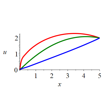
The solution in the calculus of variations (i.e. α=1\alpha=1) is the cycloid with the parametric equations x=r⁡(θ−s​i​n​θ)x=r(\theta-sin\theta) and u⁡(x)=r⁡(1−c​o​s​θ)u(x)=r(1-cos\theta). It can be displayed by the path traced out by a point placed on a rolling wheel of radius rr when it rotates by an angle θ\theta. The general solution to the ODE when α≠1\alpha\neq 1 is challenging. For example, it is easy to check that u⁡(x)=1α−1​xu(x)=\frac{1}{\sqrt{\alpha-1}}x is a stationary straight line. According to the second variation test in Eq. 25, it is a minimum when α=2\alpha=2 and x>0x>0, in this case the second variation 1δ​∫ab((x​h′​(x)−h⁡(x))2+h⁡(x))/x3​𝑑x>0\frac{1}{\delta}\int_{a}^{b}((xh^{\prime}(x)-h(x))^{2}+h(x))/x^{3}dx>0. We solve the ODE numerically, using the midpoint method of Maple for three values of α\alpha and two different initial conditions (see Fig. 2). Note that the solution resembles the Trochoid at different distances from the center of a circle of some radius.
Refer to caption

a Refer to captionb

Figure 2: Numerical solution to Brachistochrone with the initial condition: a) u(0)=0 and u(5)=2, b) u(0)=1 and u(5)=1, α=1\alpha=1 (Red), α=2\alpha=2 (Green), c) α=8\alpha=8 (Blue).

We consider another problem related to the Snell’s law governing the refraction of light in its passage from one medium to another, provided that the observed refractive index of the medium is identified with the inverse of speed c−1​(x)c^{-1}(x). Pierre de Fermat observed that Snell’s law stems from the principle that light travels the path that takes the least amount of time. Specifically, the functional F(x,u,u′)F(x,u,u^{{}^{\prime}}) is the time taken to cover the path u⁡(x)u(x) for x∈[a,b]x\in[a,b], i.e F⁡(x,u,u′)=1+u′2c⁡(x)F(x,u,u^{\prime})=\frac{\sqrt{1+u^{\prime 2}}}{c(x)} and c⁡(x)>0c(x)>0. The terms involved in Eq. 21 are ∂F(x,u,u′)∂u=0\frac{\partial F(x,u,u^{{}^{\prime}})}{\partial u}=0, ∂F(x,u,u′)∂u′=u′c2(x)F(x,u,u′)\frac{\partial F(x,u,u^{{}^{\prime}})}{\partial u^{{}^{\prime}}}=\frac{u^{\prime}}{c^{2}(x)F(x,u,u^{{}^{\prime}})}, dF(x,u,u′)d​x=u′​u′′c2(x)F(x,u,u′)−c′​(x)c⁡(x)F(x,u,u′)\frac{dF(x,u,u^{{}^{\prime}})}{dx}=\frac{u^{\prime}u^{\prime\prime}}{c^{2}(x)F(x,u,u^{{}^{\prime}})}-\frac{c^{\prime}(x)}{c(x)}F(x,u,u^{{}^{\prime}}), and dd​x​∂F(x,u,u′)∂u′=−u′​(x)​c′​(x)c3(x)F(x,u,u′)+u′′​(x)c4(x)F3(x,u,u′)\frac{d}{dx}\frac{\partial F(x,u,u^{{}^{\prime}})}{\partial u^{{}^{\prime}}}=\frac{-u^{\prime}(x)c^{\prime}(x)}{c^{3}(x)F(x,u,u^{{}^{\prime}})}+\frac{u^{\prime\prime}(x)}{c^{4}(x)F^{3}(x,u,u^{{}^{\prime}})}. Eq. 21 is rewritten as:

F(x,u,u′)(−u′​(x)​c′​(x)c3(x)F(x,u,u′)+u′′​(x)c4(x)F3(x,u,u′))−(α−1)u′c2(x)F(x,u,u′)(u′​u′′c2(x)F(x,u,u′)−c′​(x)c⁡(x)F(x,u,u′))=0F(x,u,u^{{}^{\prime}})(\frac{-u^{\prime}(x)c^{\prime}(x)}{c^{3}(x)F(x,u,u^{{}^{\prime}})}+\frac{u^{\prime\prime}(x)}{c^{4}(x)F^{3}(x,u,u^{{}^{\prime}})})-(\alpha-1)\frac{u^{\prime}}{c^{2}(x)F(x,u,u^{{}^{\prime}})}(\frac{u^{\prime}u^{\prime\prime}}{c^{2}(x)F(x,u,u^{{}^{\prime}})}-\frac{c^{\prime}(x)}{c(x)}F(x,u,u^{{}^{\prime}}))=0 (36)

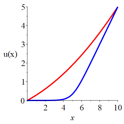
Eq. 36 can be rewritten as ∂F(x,u,u′)∂u′=k\frac{\partial F(x,u,u^{{}^{\prime}})}{\partial u^{{}^{\prime}}}=k, where kk is a constant when α=1\alpha=1 because u⁡(x)u(x) is an ignorable coordinate. It follows that the derivative of the stationary curve is u′(x)=∓kc(x)/1−k2​c2​(x)u^{\prime}(x)=\mp kc(x)/\sqrt{1-k^{2}c^{2}(x)}. For example, consider c⁡(x)=xc(x)=x and k≠0k\neq 0, then u(x)=∓1−k2​x2/k+pu(x)=\mp\sqrt{1-k^{2}x^{2}}/k+p, which is the circle (u⁡(x)−p)2+x2=k−2(u(x)-p)^{2}+x^{2}=k^{-2}. This is well-known solution in the calculus of variations. When α=0\alpha=0, Eq. 27 is rewritten as u′′​(x)​(1−u′2​(x))=0u^{\prime\prime}(x)(1-u^{\prime 2}(x))=0. The case u′2​(x)=1u^{\prime 2}(x)=1 is a particular case of the u′′​(x)=0u^{\prime\prime}(x)=0, the stationary curve u⁡(x)u(x) solution to the last ODE is independent of the speed; u⁡(x)=s​x+du(x)=sx+d. The second variation in Eq.31, ∂2F∂u2=∂2F∂u​∂u′=∂F∂u=0\frac{\partial^{2}F}{\partial u^{2}}=\frac{\partial^{2}F}{\partial u\partial u^{\prime}}=\frac{\partial F}{\partial u}=0, is (1−s2)​∫abh′2​(x)​𝑑x/δ​(s2+1)2(1-s^{2})\int_{a}^{b}h^{\prime 2}(x)dx/\delta(s^{2}+1)^{2}. The second variation is positive when s2<1s^{2}<1 because h⁡(x)h(x) cannot be a constant, and therefore the stationary curve is a minimum in this case. In other words, only straight lines with slopes in ]−1,1[]-1,1[ are minimums. When α=2\alpha=2, we can rewrite the ODE in Eq. 36 as dd​xF(x,u,u′)∂F(x,u,u′)∂u′=0\frac{d}{dx}F(x,u,u^{{}^{\prime}})\frac{\partial F(x,u,u^{{}^{\prime}})}{\partial u^{\prime}}=0; that is F(x,u,u′)∂F(x,u,u′)∂u′=kF(x,u,u^{{}^{\prime}})\frac{\partial F(x,u,u^{{}^{\prime}})}{\partial u^{\prime}}=k and therefore u′​(x)=k​c2​(x)u^{\prime}(x)=kc^{2}(x). Let us set c⁡(x)=xc(x)=x, then u⁡(x)=k​x3/3+pu(x)=kx^{3}/3+p. It is a minimum because the second variation test in Eq. 25 leads to 2​∫abh′2​(x)x2/δ​𝑑x>02\int_{a}^{b}\frac{h^{\prime 2}(x)}{x^{2}}/\delta dx>0. If we consider that there are two mediums, having different refractive indexes whose variation is smooth along the x-axis. The speed function c⁡(x)=eβ⁡(x−x0)/(1+eβ⁡(x−x0))c(x)=\sqrt{e^{\beta(x-x_{0})}/(1+e^{\beta(x-x_{0})})}, where β\beta and x0x_{0} are parameters describes two mediums. By considering this speed function, the stationary curve u⁡(x)=k​l​n​(1+eβ⁡(x−x0))/β+pu(x)=kln(1+e^{\beta(x-x_{0})})/\beta+p is a minimum because the second variation test in Eq. 25 is rewritten as 2​∫abh′2​(x)​1+eβ⁡(x−x0)eβ⁡(x−x0)​𝑑x>02\int_{a}^{b}h^{\prime 2}(x)\sqrt{\frac{1+e^{\beta(x-x_{0})}}{e^{\beta(x-x_{0})}}}dx>0, where ww is a positive function of aa, bb, and k2k^{2}. This curve u⁡(x)u(x) is plotted in Fig. 3.

Refer to caption

a Refer to captionb

Figure 3: Fast path, k=1k=1, and x0=5x_{0}=5. a) The speed is a logistic function centered on x0x_{0} and having the slope β=2\beta=2. b) The curves u(x) when the slopes are β=0.2\beta=0.2 (Red), β=2\beta=2 (blue).

6 Conclusion

In this document, the calculus of variations is revisited from a new angle. Instead of the usual variational formulation, functional centrality based on Hölder’s mean is used. For a given problem, the solution is a family of curves, where each one corresponds to a certain data selection criterion induced by the centrality measure used. Some of these solutions cannot be obtained with the usual variational formulation. To illustrate, the fastest and shortest paths are studied.

References

  • [1] D. Ziou. Pythagorean Centrality for Data Selection. arXiv preprint arXiv:2301.10010, 2023.
  • [2] R. Courant and D. Hilbert. Methods of Mathematical Physics. New York Interscience Publishers, 1953.
  • [3] G.P. Benhama, C. Cohen, E. Brunet, and C. Clanet. Brachistochrone on a velodrome. Proc. of the Royal Society A, 2020.
  • [4] F. Kerouh, D. Ziou, and K.N. Lahmar. Content-based computational chromatic adaptation. Pattern Anal. Applic. 21, pp. 1109–1120, 2018.