Type-Aware Decomposed Framework
for Few-Shot Named Entity Recognition

Yongqi Li Affiliation: School of Computer Science, Wuhan University, China Yu Yu Affiliation: School of Computer Science, Wuhan University, China Tieyun Qian Thanks: Corresponding author. Affiliation: School of Computer Science, Wuhan University, China Affiliation: Intellectual Computing Laboratory for Cultural Heritage, Wuhan University, China{liyongqi,Yu.Yu1024,qty}@whu.edu.cn

Abstract

Despite the recent success achieved by several two-stage prototypical networks in few-shot named entity recognition (NER) task, the over-detected false spans at the span detection stage and the inaccurate and unstable prototypes at the type classification stage remain to be challenging problems. In this paper, we propose a novel Type-Aware Decomposed framework, namely TadNER, to solve these problems. We first present a type-aware span filtering strategy to filter out false spans by removing those semantically far away from type names. We then present a type-aware contrastive learning strategy to construct more accurate and stable prototypes by jointly exploiting support samples and type names as references. Extensive experiments on various benchmarks prove that our proposed TadNER framework yields a new state-of-the-art performance. ¹¹ 1 Our code and data will be available at https://github.com/NLPWM-WHU/TadNER.

1 Introduction

Named entity recognition (NER) aims to detect entity spans and classify them into pre-defined categories (entity types). When there are sufficient labeled data, deep learning-based methods Huang et al. 2015; Ma and Hovy 2016; Lample et al. 2016; Chiu and Nichols 2016 can get impressive performance. In real applications, it is desirable to recognize new categories which are unseen in training/source domain. However, collecting extra labeled data for these new types will be surely time-consuming and labour-expensive. Consequently, few-shot NER Fritzler et al. 2019; Yang and Katiyar 2020, which involves identifying unseen entity types based on a few labeled samples for each class (i.e., support samples) in test domain, has attracted great research interests in recent years.

End-to-end metric learning based methods Yang and Katiyar 2020; Das et al. 2022 are the mainstream in few-shot NER. These methods need to simultaneously learn the complex structure consisting of entity boundary and entity type. When the domain gap is large, their performance will drop dramatically because it is extremely hard to capture such complicated structure information with only a few support examples for domain adaptation. This leads to the insufficient learning of boundary information, resulting that these methods often misclassify entity boundaries and cannot obtain very satisfying performance.

Recently, there is an emerging trend in adopting two-stage prototypical networks Wang et al. 2022; Ma et al. 2022c for few-shot NER, which decompose NER into two separate span extraction and type classification tasks and perform one task at each stage. Since decomposed methods only need to handle one single boundary detection task at the first stage, they can find more accurate boundaries and obtain better performance than end-to-end approaches.

Refer to caption — Figure 1: (a) shows over-detected false spans, (b) shows spans got by adopting our type-aware span filtering strategy. (c) shows inaccurate and unstable prototypes, (d) shows prototypes got by adopting our type-aware contrastive learning strategy.

While making good progress, these two-stage prototypical networks still face two challenging problems, i.e., the over-detected false spans and the inaccurate and unstable prototypes in corresponding stages. (1) At the span extraction stage in test phase, the decomposed approaches usually recall many over-detected false spans whose types only exist in the source domain. For example, “1976” in Figure 1 (a) belongs to a DATE type in the source domain since there are many samples like “Obama was born in 1961” in training, and thus it is easily recognized as a span by the span detector. However, there is no such label in the test domain and “1976” is thus assigned a false LOC type. (2) The prototypical networks in decomposed methods target at learning a type-agnostic metric similarity function to classify entities in test samples (i.e., query samples) via their distance to prototypes. Since the prototypes are constructed using very few support samples in the type-agnostic feature space, they might be inaccurate and unstable. For example, in Figure 1 (c), a prototype is just the support sample in one-shot NER and thus deviates far away from the real class center.

Based on the above observations, we propose a Type-Aware Decomposed framework, namely TadNER, for few-shot NER. Our method follows the span detection and type classification learning scheme in the decomposed framework but moves two steps further to overcome the aforementioned issues.

Firstly, we present a type-aware span filtering strategy to filter out false spans by removing those semantically far away from type names ²² 2 Note that though type assignments are unknown in few-shot NER, the type names (labels) in test domain are provided.. By this means, the over-detected spans like “1976” whose types do not exist in test domain can be removed due to the long semantic distance to type names, as shown in Figure 1 (b).

Secondly, we present a type-aware contrastive learning strategy to construct more accurate and stable prototypes by jointly leveraging type names and support samples as references. Through this way, the type names can serve as the guidance for prototypes and make them not deviate too far away from the class centers even in some extreme outlier cases, as shown in Figure 1 (d).

Extensive experimental results on 5 benchmark datasets demonstrate the superiority of our TadNER over the state-of-the-art decomposed methods. In particular, in the hard intra Few-NERD and 1-shot Domain Transfer settings, TadNER achieves a 8% and 9% absolute F1 increase, respectively.

2 Method

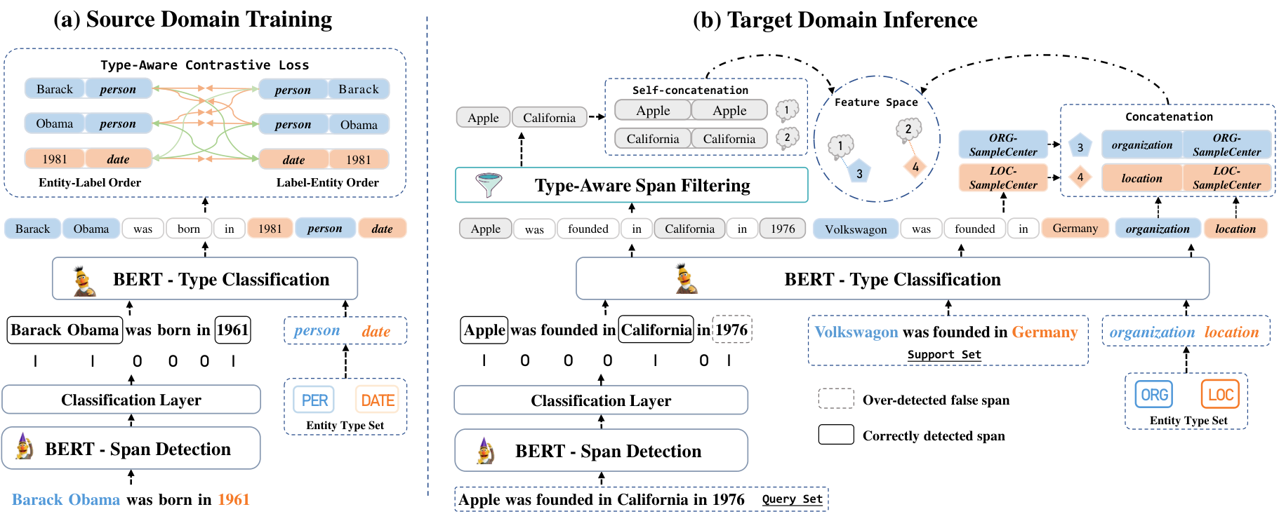
In this section, we formally present our proposed TadNER. The overall structure of our TadNER is shown in Figure 2. Note that the type-aware contrastive learning and type-aware span filtering strategies take effect at the type classification stage in the training and test domain, respectively.

Task Formulation

Given a sequence $X=\{x_{1},x_{2},...,x_{N}\}$ with $N$ tokens, NER aims to assign each token $x_{i}$ a corresponding label $y_{i}\in\mathcal{T}\cup\{\textsc{O}\}$ , where $\mathcal{T}$ is the entity type set and O denotes the non-entity label. For few-shot NER, a model is trained in a source domain dataset $\mathcal{D}_{source}$ with the entity type set $\mathcal{T}_{source}=\{t_{1},t_{2},...t_{m}\}$ . The model is then fine-tuned in a test/target domain dataset $\mathcal{D}_{target}$ with the entity type set $\mathcal{T}_{target}=\{t_{1},t_{2},...t_{n}\}$ using a given support set $\mathcal{S}_{target}$ . The entity token set and corresponding label set in $\mathcal{S}_{target}$ are denoted as $E^{s}=\{e^{s}_{1},e^{s}_{2},...,e^{s}_{M}\}$ and $Y^{s}=\{y^{s}_{1},y^{s}_{2},...,y^{s}_{M}\}$ , where $y^{s}_{i}\in\mathcal{T}_{target}$ is the label and $M$ is the number of entity tokens. The model is supposed to recognize entities in the query set $\mathcal{Q}_{target}$ of the target domain. Besides, $\mathcal{T}_{source}$ and $\mathcal{T}_{target}$ have no or very little overlap, making few-shot NER very challenging. More specifically, in the $n$ -way $k$ -shot setting, there are $n$ labels in $\mathcal{T}_{target}$ and $k$ examples associated with each label in the support set $\mathcal{S}_{target}$ .

2.1 Source Domain Training

The source domain training consists of span detection and type classification stages. The procedure is shown in Figure 2 (a).

2.1.1 Span Detection

The span detection stage is formulated as a sequence labeling task, similar to an existing decomposed NER model Ma et al. 2022c. We adopt BERT Devlin et al. 2019 with parameters ${\theta_{1}}$ as the PLM encoder $f_{\theta_{1}}$ . Given an input sentence $X=\{x_{1},x_{2},...,x_{N}\}$ , the encoder produces contextualized representations for each token as:

\mathbf{H}=[\mathbf{{h}_{1}},...,\mathbf{{h}_{N}}]=f_{\theta_{1}}([x_{1},...,x_{N}]),

(1)

where $\mathbf{H}\in\mathbb{R}^{N*r}$ ³³ 3 In this paper, $r$ denotes the hidden size of the PLM.. $\mathbf{H}$ is then fed into a classification layer consisting of a dropout layer Srivastava et al. 2014 and a linear layer to get the probability distribution $\mathbf{P}=[\mathbf{p(x_{1})},...,\mathbf{p(x_{N})}]$ ( $\mathbf{p(x_{i})}\in\mathbb{R}^{|C|}$ , $C=\{I,O\}$ ) ⁴⁴ 4 In Appendix A.6, we perform a detailed analysis using the IO, BIO, and BIOES tagging schemes. using a softmax function:

\mathbf{p(x_{i})}=softmax(Dropout(\mathbf{W}\cdot\mathbf{h_{i}}+\mathbf{b})),

(2)

where $\mathbf{W}\in\mathbb{R}^{|C|*r}$ and $\mathbf{b}\in\mathbb{R}^{|C|}$ are the weight matrix and bias.

After that, the training loss is formulated by the averaged cross-entropy of the probability distribution and the ground-truth labels:

\mathcal{L}_{span}=\frac{1}{N}\sum_{i=1}^{N}CrossEntropy(y_{i},\mathbf{p(x_{i})}),

(3)

where $y_{i}$ = $0$ when the $i$ -th token is O-token, $y_{i}$ = $1$ otherwise. Specifically, we denote the training loss of span detection stage as $\mathcal{L}_{span}$ . During the training procedure, the parameters $\{\theta_{1},\mathbf{W},\mathbf{b}\}$ are updated to minimize $\mathcal{L}_{span}$ .

2.1.2 Type Classification

Representation

Given an input sentence $X$ , we only select entity-tokens $E=\{e_{1},e_{2},...,e_{M}\}$ ( $E\subset X$ ) with ground-truth labels $Y=\{y_{1},y_{2},...,y_{M}\}$ for the training of this stage. For the entity type set $\mathcal{T}_{source}=\{t_{1},t_{2},...,t_{m}\}$ of the source domain $D_{source}$ , we manually convert them into their corresponding type names $\mathcal{T}_{source}^{{}^{\prime}}=\texttt{Map}(\mathcal{T}_{source})=\{t_{1}^{{}^{\prime}},t_{2}^{{}^{\prime}},...,t_{m}^{{}^{\prime}}\}$ ⁵⁵ 5 Map() is the function used to convert a label to a type name, e.g. “PER” to “person”. Please refer to Appendix A.7 for type names of all datasets..

After that, to obtain tokens with type name information, which are further used for calculating contrastive loss, we concatenate entity tokens with their corresponding labels in two orders, i.e., entity-label order and label-entity order. Here we use another encoder $f_{\theta_{2}}$ with parameters ${\theta_{2}}$ to obtain contextual representations:

\mathbf{h^{el}_{i}}=f_{\theta_{2}}(e_{i})\oplus f_{\theta_{2}}(\texttt{Map}(y_{i}))

(4)

\mathbf{h^{le}_{i}}=f_{\theta_{2}}(\texttt{Map}(y_{i}))\oplus f_{\theta_{2}}(e_{i}),

(5)

where $\oplus$ is the concatenation operator, and $\mathbf{h^{el}_{i}}$ and $\mathbf{h^{le}_{i}}$ denote two kinds of type-aware representations of the entity-token $e_{i}$ , which are obtained in entity-label order and label-entity order, respectively.

Type-Aware Contrastive Learning

To learn a generalized and type-aware feature space, which can further be used for constructing more accurate and stable prototypes, we borrow the idea of contrastive learning Khosla et al. 2020 and use two kinds of type-aware token representations mentioned above to construct positive and negative pairs as shown in Figure 2 (a), i.e., those with the same label in different orders as positive pairs and those with different labels as negative pairs. The type-aware contrastive loss is calculated as:

\mathcal{L}_{type}=-\sum_{i=1}^{M}\log\frac{\frac{1}{\|Z_{i}\|}\sum\limits_{z\in Z_{i}}\exp(sim(\mathbf{h_{i}^{el}},\mathbf{h_{z}^{le}})/\tau)}{\sum\limits_{j=1}^{M}\exp(sim(\mathbf{h_{i}^{el}},\mathbf{h_{j}^{le}})/\tau)},

(6)

Z_{i}=\{z~|~1\leq z\leq M,y_{z}=y_{i}\},

(7)

sim(\mathbf{h_{i}^{el}},\mathbf{h_{j}^{le}})=\frac{\mathbf{h_{i}^{el}}\cdot\mathbf{h_{j}^{le}}^{\mathsf{T}}}{\sum_{k=1}^{M}{(\mathbf{h_{k}^{el}}\cdot\mathbf{h_{j}^{le}}^{\mathsf{T}})}},

(8)

where $M$ is the number of entity tokens in a batch and $Z_{i}$ is the set of positive samples with the same label type $y_{i}$ . Here we adopt the dot product with a normalization factor as the similarity function $sim()$ . We also add a temperature hyper-parameter $\tau$ for focusing more on difficult pairs Chen et al. 2020. During the source domain training, the parameters $\theta_{2}$ are updated to minimize $\mathcal{L}_{type}$ .

2.2 Target Domain Inference

As illustrated in Figure 2 (b), during the target domain inference, we first extract candidate spans in query sentences and then remove over-detected false spans via the type-aware span filtering strategy. Finally, we classify remaining candidate spans into certain entity types to get the final results.

2.2.1 Span Detection

The span detector with its parameters $\{\theta_{1},\textbf{W},\textbf{b}\}$ trained in the source domain is further fine-tuned with samples in the support set $\mathcal{S}_{target}$ in the target domain to minimize $\mathcal{L}_{span}$ in Eq.(3). To alleviate the risk of over-fitting, we adopt a loss-based early stopping strategy, i.e., stopping the fine-tuning procedure once the loss rises $\beta$ times continuously, where $\beta$ is a hyper-parameter.

After fine-tuning the span detector, we use it to detect entity words of query sentences in $\mathcal{Q}_{target}$ and then consider continuous entity words as a candidate span, e.g., “Barack Obama”. Finally, we obtain the candidate span set $C_{span}$ containing all candidate spans, which will be assigned entity types at the type classification stage.

2.2.2 Type Classification

Domain Adaption

Benefiting from the generalized and type-aware feature space trained in the source domain, we can further get a domain-specific encoder $f_{\theta_{2}^{{}^{\prime}}}$ via fine-tuning with the following loss:

\mathcal{L}_{label}=\frac{1}{M}\sum_{i=1}^{M}\frac{s(e^{s}_{i},\texttt{Map}(y^{s}_{i}))}{\sum\limits_{t_{j}\in\mathcal{T}_{target}}s(e^{s}_{i},\texttt{Map}(t_{j}))},

(9)

s(p,q)=f_{\theta_{2}}(p)\cdot f_{\theta_{2}}(q)^{\mathsf{T}}.

(10)

Type-Aware Span Filtering

As we illustrate in the introduction, the span detector may generate some over-detected false spans whose type names only belong the source domain, since the semantics of entity type names are not considered at the span detection stage. To solve this problem, we propose a type-aware span filtering strategy during the inference phase to remove these false spans. Intuitively, the semantic distance of these false spans is far from all the golden type names. Based on this assumption, we calculate a threshold $\gamma_{t}$ with the fine-tuned encoder $f_{\theta_{2}^{{}^{\prime}}}$ using entity tokens and corresponding type names in the support set:

\gamma_{t}=\min\limits_{1\leq i\leq M}f_{\theta_{2}^{{}^{\prime}}}(e_{i}^{s})\cdot f_{\theta_{2}^{{}^{\prime}}}(\texttt{Map}(y_{i}^{s}))^{\mathsf{T}}.

(11)

This threshold $\gamma_{t}$ is used to remove the over-detected false spans. And the remaining candidate spans will be assigned corresponding labels.

Type-Aware Prototype Construction

We can construct a type-aware prototype for each entity type $t_{j}\in\mathcal{T}_{target}$ , which is more accurate and stable owing to the generalized and type-aware feature space learned in the source domain:

\mathbf{p_{j}}=f_{\theta_{2}^{{}^{\prime}}}(\texttt{Map}(t_{j}))\oplus\frac{1}{\|Z_{j}\|}\sum\limits_{i\in Z_{j}}f_{\theta_{2}^{{}^{\prime}}}(e^{s}_{i}),

(12)

Z_{j}=\{i~|~1\leq i\leq M,y^{s}_{i}=t_{j}\},

(13)

where $\oplus$ is the concatenation operator and $Z_{j}$ denotes the set of entity words with the label type $t_{j}$ in the support set.

Inference

For each remaining candidate span $s_{i}$ , we assign it a label type $t_{j}\in\mathcal{T}_{target}$ with the highest similarity:

y_{pred}=\mathop{\arg\max}\limits_{t_{j},t_{j}\in\mathcal{T}_{target}}(\mathbf{h_{i}}\cdot\mathbf{p_{j}}^{\mathsf{T}}),

(14)

\mathbf{h_{i}}=f_{\theta_{2}^{{}^{\prime}}}(s_{i})\oplus f_{\theta_{2}^{{}^{\prime}}}(s_{i}),

(15)

where $\mathbf{p_{j}}$ is the type-aware prototype representation corresponding to the label type $t_{j}$ , and $y_{pred}$ is the predicted label type of the candidate span $s_{i}$ . $\mathbf{h_{i}}$ is the self-concatenated representation of $s_{i}$ for consistency with the dimension of the prototype $\mathbf{p_{j}}$ . The entire procedure of inference in the target domain is presented in Appendix A.1.

Paradigms	Models	Intra					Inter
		1 $\sim$ 2-shot		5 $\sim$ 10-shot		Avg.	1 $\sim$ 2-shot		5 $\sim$ 10-shot		Avg.
		5 way	10 way	5 way	10 way	Avg.	5 way	10 way	5 way	10 way	Avg.
One-stage	ProtoBERT^†	20.76±0.84	15.05±0.44	42.54±0.94	35.40±0.13	28.44	38.83±1.49	32.45±0.79	58.79±0.44	52.92±0.37	45.75
	NNShot^†	25.78±0.91	18.27±0.41	36.18±0.79	27.38±0.53	26.90	47.24±1.00	38.87±0.21	55.64±0.63	49.57±2.73	47.83
	StructShot^†	30.21±0.90	21.03±1.13	38.00±1.29	26.42±0.60	28.92	51.88±0.69	43.34±0.10	57.32±0.63	49.57±3.08	50.53
	FSLS^∗	30.38±2.85	28.31±4.03	46.85±3.49	40.76±3.18	36.58	44.52±4.59	44.01±3.35	59.74±2.51	56.67±1.75	51.24
	CONTaiNER^∗	41.51±0.07	36.62±0.04	57.83±0.01	51.04±0.24	46.75	50.92±0.29	47.02±0.24	63.35±0.07	60.14±0.16	55.36
Two-stage	ESD^†	36.08±1.60	30.00±0.70	52.14±1.50	42.15±2.60	40.09	59.29±1.25	52.16±0.79	69.06±0.80	64.00±0.43	61.13
	DecomposedMetaNER^†	49.48±0.85	42.84±0.46	62.92±0.57	57.31±0.25	53.14	64.75±0.35	58.65±0.43	71.49±0.47	68.11±0.05	65.75
	TadNER	60.78±0.32	55.44±0.08	67.94±0.17	60.87±0.22	61.26	64.83±0.14	64.06±0.19	72.12±0.12	69.94±0.15	67.74

Table 1: F1 scores with standard deviations for Few-NERD. ^† denotes the results reported by Ma et al. 2022c. ^∗ denotes the results reported by our replication using data of the same version. The best results are in bold and the second best ones are underlined.

Paradigms	Models	1-shot					5-shot
Paradigms	Models	I2B2	CoNLL	WNUT	GUM	Avg.	I2B2	CoNLL	WNUT	GUM	Avg.
One-stage	ProtoBERT^†	13.4±3.0	49.9±8.6	17.4±4.9	17.8±3.5	24.6	17.9±1.8	61.3±9.1	22.8±4.5	19.5±3.4	30.4
	NNShot^†	15.3±1.6	61.2±10.4	22.7±7.4	10.5±2.9	27.4	22.0±1.5	74.1±2.3	27.3±5.4	15.9±1.8	34.8
	StructShot^†	21.4±3.8	62.4±10.5	24.2±8.0	7.8±2.1	29.0	30.3±2.1	74.8±2.4	30.4±6.5	13.3±1.3	37.2
	FSLS^∗	18.3±3.5	50.9±6.5	14.3±5.5	12.6±2.8	24.0	25.4±2.7	63.9±3.3	24.0±3.2	18.8 ±2.2	33.1
	CONTaiNER^†	21.5±1.7	61.2±10.7	27.5±1.9	18.5±4.9	32.2	36.7±2.1	75.8±2.7	32.5±3.8	25.2±2.7	42.6
Two-stage	DecomposedMetaNER^∗	15.5±3.0	61.2±9.2	27.7±5.3	20.3±4.2	31.2	19.8±2.6	75.2±5.8	29.8±3.9	33.5±2.4	39.6
Two-stage	TadNER	39.3±3.8	70.4±10.6	32.8±4.8	24.2±4.1	41.7	45.2±2.3	80.5±3.6	34.5±4.6	35.1±2.2	48.8

Table 2: F1 scores with standard deviations for Domain Transfer. ^† denotes the results reported by Das et al. 2022. ^∗ denotes the results reported by our replication. Since no previous two-stage methods have conducted experiments under this setting, we choose the strong DecomposedMetaNER for reproduction experiments, and ^∗ denotes the results reported by our replication. The best results are in bold and the second best ones are underlined.

3 Experiments

3.1 Evaluation Protocal

Datasets

Ding et al. 2021 propose a large scale dataset Few-NERD for few-shot NER, which contains 66 fine-grained entity types across 8 coarse-grained entity types. It contains intra and inter tasks where the train/dev/test sets are divided according to the coarse-grained and fine-grained types, respectively. Besides, following Das et al. 2022, we also conduct Domain Transfer experiments, where data are from different text domains (e.g., Wiki, News). We take OntoNotes (General) Weischedel et al. 2013 as our source domain, and evaluate few-shot performances on I2B2 (Medical) Stubbs and Uzuner 2015, CoNLL (News) Tjong Kim Sang and De Meulder 2003, WNUT (Social) Derczynski et al. 2017 and GUM Zeldes 2017 datasets.

Baselines

We compare our proposed TadNER with many strong baselines, including one-stage and two-stage types. The one-stage baselines include ProtoBERT Snell et al. 2017, NNShot Yang and Katiyar 2020, StructShot Yang and Katiyar 2020, FSLS Ma et al. 2022a and CONTaiNER Das et al. 2022. Note that FSLS also adopts type names. The two-stage baselines include ESD Wang et al. 2022 and the DecomposedMetaNER Ma et al. 2022c ⁶⁶ 6 Please refer to Appendix A.2-A.5 for more descriptions about datasets, evaluation methods, baselines and implementation details..

3.2 Main Results

Table 1 and 2 report the comparison results between our method and baselines under Few-NERD ⁷⁷ 7 Results are tested with the latest version of data from https://ningding97.github.io/fewnerd/, which is corresponding with https://github.com/microsoft/vert-papers/tree/master/papers/DecomposedMetaNER#few-nerd-arxiv-v6-version. and Domain Transfer, respectively. We have the following important observations: 1) Our model demonstrates superiority under Few-NERD settings. Notably, in the more challenging intra task, our TadNER achieves an average 8.2% increase in F1 score. Besides, our model outperforms baselines by 10.5% and 9.2% under 1-shot and 5-shot Domain Transfer settings, respectively. 2) Particularly, when provided with very few samples (e.g., 1-shot), the improvements become even more significant, which is a very attractive property. 3) The performance of DecomposedMetaNER, a competing model, severely deteriorates under certain settings, such as I2B2. This is primarily due to the presence of numerous sentences without entities, leading to multiple false detected spans. In contrast, our TadNER effectively mitigates this issue through the type-aware span filtering strategy, successfully removing false spans and achieving promising results.

Figure 3: Case study. C1 and C2 are from Few-NERD intra and CoNLL2003 in Cross datasets, respectively, and organization-sportsteam, organization-sportsleague, ORG and LOC are entity types.

3.3 Ablation Study

To validate the effectiveness of the main components in TadNER, we introduce the following variant baselines for the ablation study: 1) TadNER w/o Type-Aware Span Filtering (TASF) removes the type-aware span filtering strategy and directly feeds all spans detected at span detection stage to type classification. 2) TadNER w/o Type Names (TN) further replaces type names with random vectors when calculating contrastive loss and constructs class prototypes using only the support samples. 3) TadNER w/o Span-Finetune skips the target domain adaptation of the span detection stage. 4) TadNER w/o Type-Finetune skips the target domain adaptation of the type classification stage.

Models	1-shot				5-shot				Avg.
Models	I2B2	CoNLL	WNUT	GUM	I2B2	CoNLL	WNUT	GUM	Avg.
TadNER	39.3	70.4	32.8	24.2	45.2	80.5	34.5	35.1	45.3
w/o TASF	21.2	68.5	31.6	24.2	27.4	80.1	34.3	35.1	40.3
w/o TN	20.0	65.6	28.3	20.3	26.2	76.3	33.8	33.2	38.0
w/o Span-Finetune	37.0	52.5	30.7	15.0	40.1	50.8	31.7	16.2	34.3
w/o Type-Finetune	37.6	68.3	32.3	20.3	45.2	76.3	33.6	27.9	42.7

Table 3: Results (F1 scores) for ablation study under Domain Transfer settings. The best results are in bold.

From Table 3, we can observe that: 1) The removal of the type-aware span filtering strategy leads to a drop in performance across most cases, particularly in entity-sparse datasets like I2B2, where a large number of false positive spans are detected. Besides, for entity-dense datasets like GUM, the performance is not harmed by the span filtering strategy, which proves the robustness and effectiveness of our model in various real-world applications. 2) The omission of type names also results in a significant decrease in performance, indicating that our model indeed learns a type-aware feature space, which plays a crucial role in few-shot scenarios. 3) The elimination of finetuning in the span detection and type classification stages exhibits a substantial performance drop. This demonstrates that the training objective in the source domain training phase aligns well with the target domain finetuning phase via task decomposition and contrastive learning strategy, despite having different entity classes. As a result, the model can effectively utilize the provided support samples from the target domain, enhancing its performance in few-shot scenarios.

3.4 Case Study

To examine how our model accurately constructs prototypes and filters out over-detected false spans with the help of type names, we randomly select one query sentence from Few-NERD intra and CoNLL2003 for case study. We compare TadNER with DecomposedMetaNER Ma et al. 2022c, which also belongs to the two-stage methods.

As shown in Figure 3, in the first case, our model correctly predicts “turkish tff third league” as “organization-sportsleague” type, while DecomposedMetaNER identifies it as a wrong “organization-sportsteam” type. Since the type name and the entity span have an overlapping word “league”, incorporating the type name into the construction of the prototype will make the identification much easier. Conversely, without the type name, it would be hard to distinguish two categories of entities because they both represent “sports-related organizations”.

In the second case, DecomposedMetaNER incorrectly identifies “two” as an entity span and then assigns it a wrong entity type “LOC”, since there are many samples like “The two sides had not met since Oct. 18” in the source domain Ontonotes, where “two” is an entity of “CARDINAL” type. In contrast, our TadNER successfully removes this false span via the type-aware span filtering strategy.

3.5 Impact of Type Names

To further explore the impact of incorporating the semantics of type names and whether model performance is sensitive to these converted type names. We perform experiments with the following variants of type names: 1) Original type names, which are used in our main comparision experiments. 2) Synonymous type names. We generate three synonyms for each original type name as variants using ChatGPT. These synonyms were automatically generated to explore the effect of different but related type names on model performance. 3) Meaningless type names, e.g., “label 1” and “label 2”. 4) Misleading type names, e.g., “person” for “LOC” and “location’ for “PER” in the CoNLL dataset. Please refer to Appendix A.7 for details.

Figure 4: F1 Scores on Few-NERD Intra and CoNLL 2003 with different variants of type names.

As shown from the Figure 4, we can make the following observations: 1) All three variants of synonym type names have comparable performance, indicating that our method is robust to different ways of transforming type names. However, the best way is still the direct transformation method, such as “person” for “PER”, which is how we obtain the original type names. 2) Irrelevant or incorrect information in meaningless and misleading type names leads to a significant degradation in model performance, indicating that the semantics associated with entity classes are more suitable as anchor points for contrastive learning.

3.6 Impact of Type-Aware Prototypes

In order to investigate the effectiveness of our proposed strategy for solving the problem of inaccurate and unstable prototypes in the type classification stage, we further perform an analysis of the impact of stability and quality of prototypes. We select three baselines as our compared methods: 1) TadNER w/o Type Names (TN) (the second variant baseline in the ablation study). 2) DecomposedMetaNER Ma et al. 2022c. 3) Vanilla Contrastive Learning (CL), which adopts token-token contrastive loss and was proposed by Das et al. 2022. We use it to train the type classification module in a decomposed NER framework, in order to explore whether it can address the issue of unstable and inaccurate prototypes. Here we adopt the same 10 samplings used in the 1-shot Domain Transfer experiments.

Figure 5: Impacts of prototypes by different methods under 1-shot Domain Transfer setting. The horizontal and vertical coordinates indicate the n-th sampling and the accuracy of type classification, respectively.

As shown in Figure 5, our proposed TadNER achieves a significant improvement over DecomposedMetaNER on each dataset and is more stable across different samplings. Besides, removing type names causes a sharp performance drop in some cases for TadNER w/o TN, indicating that the incorporation of type names indeed helps construct more stable and accurate prototypes. Moreover, Vanilla CL performs extremely poorly due to the introduction of an additional projection layer, which is a crucial component employed in various contrastive learning methods Chen et al. 2020; Das et al. 2022. However, the inclusion of this layer hampers the model’s capacity to acquire adequate semantics related to entity classification.

3.7 Error Analysis

We conduct an error analysis to examine the detailed types of errors made by different models. The error statistics are shown in Table 4.

Models	False Positive				False Negative				False
	Span		Type		Span		Type
	Num.	Ratio	Num.	Ratio	Num.	Ratio	Num.	Ratio
FSLS	990	85.4%	169	14.6%	1178	87.5%	169	12.5%	2506
CONTaiNER	881	63.3%	511	36.7%	628	55.1%	511	44.9%	2531
ESD	562	56.5%	433	43.5%	932	68.3%	433	31.7%	2360
DecomposedMetaNER	622	56.2%	485	43.8%	639	56.9%	485	43.1%	2231
TadNER	786	81.2%	182	18.8%	450	71.2%	182	28.8%	1600

Table 4: Error analysis for different methods under the Few-NERD Intra 5-way 1

\sim

2-shot setting. We select the first 300 episodes for analysis. “False Positive” and “False Negative” denote the incorrectly extracted entities and unrecalled entities, respectively. “Span” and “Type” denote the error is due to incorrect span/type.

We can observe that: 1) Our TadNER makes fewer errors than baselines overall. Notably, it significantly reduces false negatives, indicating its ability to accurately recall more correct entities. 2) Both TadNER and FSLS can effectively reduce “Type” errors by incorporating type names. However, though FSLS has less “Type” errors than our TadNER, it produces a much larger number of unrecalled samples, i.e., false negatives. 3) Our TadNER still suffers from inaccurate span prediction, which inspires our future work.

3.8 Model Efficiency

Compared to one-stage approaches, e.g., CONTaiNER, two-stage models require more parameters, longer training and inference times. To have a close look at the time cost induced by two-stage models, we perform a model efficiency analysis and show the results in Table 5.

Paradigms	Models	#Para.	Train	Adapt	Inference	F1
One-stage	FSLS	222M	1871s	10s	14ms	30.38
One-stage	CONTaiNER	112M	980s	1s	17ms	41.51
Two-stage	ESD	112M	2601s	0s	35ms	36.08
	DecomposedMetaNER	222M	35495s	2s	37ms	49.48
	TadNER	222M	3796s	1.5s	32ms	60.29

Table 5: Model efficiency analysis for different methods under the Few-NERD Intra 5-way 1

\sim

2-shot setting.

From Table 5, it can be seen that two-stage models indeed require longer training and inference time than one-stage models. However, two-stage models often get better performance. In particular, our TadNER is the most effective one among both one-stage and two-stage models, and it achieves a F1 improvement of 45% and 67% over CONTaiNER and ESD. It is also the most efficient one among three two-stage models in terms of the inference time.

3.9 Zero-Shot Performance

Since there is no domain-specific support set under zero-shot NER settings, it is extremely challenging and rarely explored. While we believe our proposed TadNER can obtain certain zero-shot ability after training in the source domain for the following two reasons: 1) the model can extract entity spans in the span detection stage before fine-tuning with support samples, 2) since the feature space learnt in the type classification stage is well generalized and type-aware, we can directly adopt the representations of type names as prototypes of novel entity types. To demonstrate the promising performance of our model under zero-shot settings, we select SpanNER Wang et al. 2021 as a strong baseline, which is a decomposed-based method and good at solving zero-shot NER problem.

Model	Domain Transfer
Model	I2B2	CoNLL	WNUT	GUM	Avg.
SpanNER (0-shot)	8.02	23.63	24.82	6.57	15.76
TadNER (0-shot)	17.13	43.14	25.06	7.62	23.24

Table 6: F1 scores under Domain Transfer zero-shot settings.

As shown in Table 6, our proposed TadNER performs better than SpanNER Wang et al. 2021 under every case. The reason for this may be that the type classification of SpanNER is based on a traditional supervised classification model, which performs worse generalization in cross-domain scenarios. Besides, compared with previous metric-based methods Das et al. 2022; Ma et al. 2022c for few-shot NER, which heavily rely on support sets and had no zero-shot capability, our method is more inspirational for future zero-shot NER works.

4 Related Work

Few-Shot NER

Few-shot NER methods can be categorized into two types: prompt-based and metric-based. Prompt-based methods focus on leveraging pre-trained language model knowledge for NER through prompt learning Cui et al. 2021; Ma et al. 2022b; Huang et al. 2022; Lee et al. 2022. They rely on templates, prompts, or good examples to utilize the pre-trained knowledge effectively. Metric-based methods aim to learn a feature space with good generalizability and classify test samples using nearest class prototypes Snell et al. 2017; Fritzler et al. 2019; Ji et al. 2022; Ma et al. 2022c or neighbor samples Yang and Katiyar 2020; Das et al. 2022.

There are also some efforts to improve few-shot NER by incorporating type name (label) semantics Hou et al. 2020; Ma et al. 2022a. These methods usually treat labels as class representatives and align tokens with them, yet neglecting the joint training of entity words and label representations. Hence they can only use either support sets or labels as class references. Instead, our method exploits support samples and type names simultaneously, which helps construct more accurate and stable prototypes in the target domain.

Task Decomposition and Contrastive Learning

Recently, decomposed-based methods have emerged as effective solutions for the NER problem Shen et al. 2021; Wang et al. 2021; Zhang et al. 2022; Wang et al. 2022; Ma et al. 2022c. These methods can learn entity boundary information well in data-limited scenarios and often get better results. However, the widely used prototypical networks in these methods may encounter inaccurate and unstable prototypes given limited support samples at the type classification stage. Besides, they may face the problem of over-detected false spans produced at the span detection stage. Our method can address these two issues via the proposed type-aware contrastive learning and type-aware span filtering strategies.

Our method is also inspired by contrastive learning Chen et al. 2020; Khosla et al. 2020. Due to its good generalization performance, two recent methods Das et al. 2022; Huang et al. 2022 borrow this idea for few-shot NER, which construct contrastive loss between tokens or between the token and the prompt. However, they are both the end-to-end approach and thus have the inherent drawback that cannot learn good entity boundary information. In contrast, our method is a decomposed one and our contrastive loss is constructed between tokens with additional type name information, which can find accurate boundary and learn a type-aware feature space.

5 Conclusion

In this paper, we propose a novel TadNER framework for few-shot NER, which handles the span detection and type classification sub-tasks at two stages. For type classification, we present a type-aware contrastive learning strategy to learn a type-aware and generalized feature space, enabling the model to construct more accurate and stable prototypes with the help of type names. Based on it, we introduce a type-aware span filtering strategy for removing over-detected false spans produced at the span detection stage. Extensive experiments demonstrate that our method achieves superior performance over previous SOTA methods, especially in the challenging scenarios. In the future, we will try to extend TadNER to other NLP tasks.

Limitations

Our proposed TadNER mainly focuses on the type classification stage of few-shot NER and simply adopt token classification for detecting entity spans. There might be better solutions, e.g., using global boundary matrix. However, due to its high GPU memory requirements, we do not include it in our current framework. This drives us to find more efficient and powerful span detector for better few-shot NER performance in the future.

Ethics Statement

Our work is entirely at the methodological level and therefore there will not be any negative social impacts. In addition, since the performance of the model is not yet at a practical level, it cannot be applied in certain high-risk scenarios (such as the I2B2 dataset used in our paper) yet, leaving room for further improvements in the future.

Acknowledgments

This work was supported by the grant from the National Natural Science Foundation of China (NSFC) project (No. 62276193). It was also supported by the Joint Laboratory on Credit Science and Technology of CSCI-Wuhan University.

References

Chen et al. (2020) Ting Chen, Simon Kornblith, Mohammad Norouzi, and Geoffrey Hinton. 2020. A simple framework for contrastive learning of visual representations. In Proceedings of the 37th International Conference on Machine Learning, volume 119 of Proceedings of Machine Learning Research, pages 1597–1607. PMLR.
Chiu and Nichols (2016) Jason P.C. Chiu and Eric Nichols. 2016. Named entity recognition with bidirectional LSTM-CNNs. Transactions of the Association for Computational Linguistics, 4:357–370.
Cui et al. (2021) Leyang Cui, Yu Wu, Jian Liu, Sen Yang, and Yue Zhang. 2021. Template-based named entity recognition using BART. In Findings of the Association for Computational Linguistics: ACL-IJCNLP 2021, pages 1835–1845, Online. Association for Computational Linguistics.
Das et al. (2022) Sarkar Snigdha Sarathi Das, Arzoo Katiyar, Rebecca Passonneau, and Rui Zhang. 2022. CONTaiNER: Few-shot named entity recognition via contrastive learning. In Proceedings of the 60th Annual Meeting of the Association for Computational Linguistics (Volume 1: Long Papers), pages 6338–6353, Dublin, Ireland. Association for Computational Linguistics.
Derczynski et al. (2017) Leon Derczynski, Eric Nichols, Marieke van Erp, and Nut Limsopatham. 2017. Results of the WNUT2017 shared task on novel and emerging entity recognition. In Proceedings of the 3rd Workshop on Noisy User-generated Text, pages 140–147, Copenhagen, Denmark. Association for Computational Linguistics.
Devlin et al. (2019) Jacob Devlin, Ming-Wei Chang, Kenton Lee, and Kristina Toutanova. 2019. BERT: Pre-training of deep bidirectional transformers for language understanding. In Proceedings of the 2019 Conference of the North American Chapter of the Association for Computational Linguistics: Human Language Technologies, Volume 1 (Long and Short Papers), pages 4171–4186, Minneapolis, Minnesota. Association for Computational Linguistics.
Ding et al. (2021) Ning Ding, Guangwei Xu, Yulin Chen, Xiaobin Wang, Xu Han, Pengjun Xie, Haitao Zheng, and Zhiyuan Liu. 2021. Few-NERD: A few-shot named entity recognition dataset. In Proceedings of the 59th Annual Meeting of the Association for Computational Linguistics and the 11th International Joint Conference on Natural Language Processing (Volume 1: Long Papers), pages 3198–3213, Online. Association for Computational Linguistics.
Fritzler et al. (2019) Alexander Fritzler, Varvara Logacheva, and Maksim Kretov. 2019. Few-shot classification in named entity recognition task. In Proceedings of the 34th ACM/SIGAPP Symposium on Applied Computing, SAC ’19, page 993–1000, New York, NY, USA. Association for Computing Machinery.
Hou et al. (2020) Yutai Hou, Wanxiang Che, Yongkui Lai, Zhihan Zhou, Yijia Liu, Han Liu, and Ting Liu. 2020. Few-shot slot tagging with collapsed dependency transfer and label-enhanced task-adaptive projection network. In Proceedings of the 58th Annual Meeting of the Association for Computational Linguistics, pages 1381–1393, Online. Association for Computational Linguistics.
Huang et al. (2022) Yucheng Huang, Kai He, Yige Wang, Xianli Zhang, Tieliang Gong, Rui Mao, and Chen Li. 2022. COPNER: Contrastive learning with prompt guiding for few-shot named entity recognition. In Proceedings of the 29th International Conference on Computational Linguistics, pages 2515–2527, Gyeongju, Republic of Korea. International Committee on Computational Linguistics.
Huang et al. (2015) Zhiheng Huang, Wei Xu, and Kai Yu. 2015. Bidirectional lstm-crf models for sequence tagging. arXiv preprint arXiv:1508.01991.
Ji et al. (2022) Bin Ji, Shasha Li, Shaoduo Gan, Jie Yu, Jun Ma, Huijun Liu, and Jing Yang. 2022. Few-shot named entity recognition with entity-level prototypical network enhanced by dispersedly distributed prototypes. In Proceedings of the 29th International Conference on Computational Linguistics, pages 1842–1854, Gyeongju, Republic of Korea. International Committee on Computational Linguistics.
Khosla et al. (2020) Prannay Khosla, Piotr Teterwak, Chen Wang, Aaron Sarna, Yonglong Tian, Phillip Isola, Aaron Maschinot, Ce Liu, and Dilip Krishnan. 2020. Supervised contrastive learning. In Advances in Neural Information Processing Systems, volume 33, pages 18661–18673. Curran Associates, Inc.
Lample et al. (2016) Guillaume Lample, Miguel Ballesteros, Sandeep Subramanian, Kazuya Kawakami, and Chris Dyer. 2016. Neural architectures for named entity recognition. In Proceedings of the 2016 Conference of the North American Chapter of the Association for Computational Linguistics: Human Language Technologies, pages 260–270, San Diego, California. Association for Computational Linguistics.
Lee et al. (2022) Dong-Ho Lee, Akshen Kadakia, Kangmin Tan, Mahak Agarwal, Xinyu Feng, Takashi Shibuya, Ryosuke Mitani, Toshiyuki Sekiya, Jay Pujara, and Xiang Ren. 2022. Good examples make a faster learner: Simple demonstration-based learning for low-resource NER. In Proceedings of the 60th Annual Meeting of the Association for Computational Linguistics (Volume 1: Long Papers), pages 2687–2700, Dublin, Ireland. Association for Computational Linguistics.
Loshchilov and Hutter (2019) Ilya Loshchilov and Frank Hutter. 2019. Decoupled weight decay regularization. In 7th International Conference on Learning Representations, ICLR 2019, New Orleans, LA, USA, May 6-9, 2019. OpenReview.net.
Ma et al. (2022a) Jie Ma, Miguel Ballesteros, Srikanth Doss, Rishita Anubhai, Sunil Mallya, Yaser Al-Onaizan, and Dan Roth. 2022a. Label semantics for few shot named entity recognition. In Findings of the Association for Computational Linguistics: ACL 2022, pages 1956–1971, Dublin, Ireland. Association for Computational Linguistics.
Ma et al. (2022b) Ruotian Ma, Xin Zhou, Tao Gui, Yiding Tan, Linyang Li, Qi Zhang, and Xuanjing Huang. 2022b. Template-free prompt tuning for few-shot NER. In Proceedings of the 2022 Conference of the North American Chapter of the Association for Computational Linguistics: Human Language Technologies, pages 5721–5732, Seattle, United States. Association for Computational Linguistics.
Ma et al. (2022c) Tingting Ma, Huiqiang Jiang, Qianhui Wu, Tiejun Zhao, and Chin-Yew Lin. 2022c. Decomposed meta-learning for few-shot named entity recognition. In Findings of the Association for Computational Linguistics: ACL 2022, pages 1584–1596, Dublin, Ireland. Association for Computational Linguistics.
Ma and Hovy (2016) Xuezhe Ma and Eduard Hovy. 2016. End-to-end sequence labeling via bi-directional LSTM-CNNs-CRF. In Proceedings of the 54th Annual Meeting of the Association for Computational Linguistics (Volume 1: Long Papers), pages 1064–1074, Berlin, Germany. Association for Computational Linguistics.
Shen et al. (2021) Yongliang Shen, Xinyin Ma, Zeqi Tan, Shuai Zhang, Wen Wang, and Weiming Lu. 2021. Locate and label: A two-stage identifier for nested named entity recognition. In Proceedings of the 59th Annual Meeting of the Association for Computational Linguistics and the 11th International Joint Conference on Natural Language Processing (Volume 1: Long Papers), pages 2782–2794, Online. Association for Computational Linguistics.
Snell et al. (2017) Jake Snell, Kevin Swersky, and Richard Zemel. 2017. Prototypical Networks for Few-shot Learning. In Advances in Neural Information Processing Systems, volume 30. Curran Associates, Inc.
Srivastava et al. (2014) Nitish Srivastava, Geoffrey Hinton, Alex Krizhevsky, Ilya Sutskever, and Ruslan Salakhutdinov. 2014. Dropout: a simple way to prevent neural networks from overfitting. The journal of machine learning research, 15(1):1929–1958.
Stubbs and Uzuner (2015) Amber Stubbs and Özlem Uzuner. 2015. Annotating longitudinal clinical narratives for de-identification: The 2014 i2b2/uthealth corpus. Journal of biomedical informatics, 58:S20–S29.
Tjong Kim Sang and De Meulder (2003) Erik F. Tjong Kim Sang and Fien De Meulder. 2003. Introduction to the CoNLL-2003 shared task: Language-independent named entity recognition. In Proceedings of the Seventh Conference on Natural Language Learning at HLT-NAACL 2003, pages 142–147.
Wang et al. (2022) Peiyi Wang, Runxin Xu, Tianyu Liu, Qingyu Zhou, Yunbo Cao, Baobao Chang, and Zhifang Sui. 2022. An enhanced span-based decomposition method for few-shot sequence labeling. In Proceedings of the 2022 Conference of the North American Chapter of the Association for Computational Linguistics: Human Language Technologies, pages 5012–5024, Seattle, United States. Association for Computational Linguistics.
Wang et al. (2021) Yaqing Wang, Haoda Chu, Chao Zhang, and Jing Gao. 2021. Learning from language description: Low-shot named entity recognition via decomposed framework. In Findings of the Association for Computational Linguistics: EMNLP 2021, pages 1618–1630, Punta Cana, Dominican Republic. Association for Computational Linguistics.
Weischedel et al. (2013) Ralph Weischedel, Martha Palmer, Mitchell Marcus, Eduard Hovy, Sameer Pradhan, Lance Ramshaw, Nianwen Xue, Ann Taylor, Jeff Kaufman, Michelle Franchini, et al. 2013. Ontonotes release 5.0 ldc2013t19. Linguistic Data Consortium, Philadelphia, PA.
Wolf et al. (2020) Thomas Wolf, Lysandre Debut, Victor Sanh, Julien Chaumond, Clement Delangue, Anthony Moi, Pierric Cistac, Tim Rault, Remi Louf, Morgan Funtowicz, Joe Davison, Sam Shleifer, Patrick von Platen, Clara Ma, Yacine Jernite, Julien Plu, Canwen Xu, Teven Le Scao, Sylvain Gugger, Mariama Drame, Quentin Lhoest, and Alexander Rush. 2020. Transformers: State-of-the-art natural language processing. In Proceedings of the 2020 Conference on Empirical Methods in Natural Language Processing: System Demonstrations, pages 38–45, Online. Association for Computational Linguistics.
Yang and Katiyar (2020) Yi Yang and Arzoo Katiyar. 2020. Simple and effective few-shot named entity recognition with structured nearest neighbor learning. In Proceedings of the 2020 Conference on Empirical Methods in Natural Language Processing (EMNLP), pages 6365–6375, Online. Association for Computational Linguistics.
Zeldes (2017) Amir Zeldes. 2017. The gum corpus: Creating multilayer resources in the classroom. Lang. Resour. Eval., 51(3):581–612.
Zhang et al. (2022) Xinghua Zhang, Bowen Yu, Yubin Wang, Tingwen Liu, Taoyu Su, and Hongbo Xu. 2022. Exploring modular task decomposition in cross-domain named entity recognition. In Proceedings of the 45th International ACM SIGIR Conference on Research and Development in Information Retrieval, pages 301–311.

Appendix A Appendix

A.1 Target Domain Inference Algorithm

Algorithm 1 describes the process of domain adaptation using support set in the target domain and prediction on the query set. Lines 1-7 describe the target domain adaptation process for the span detection stage. Lines 8-14 describe the target domain adaptation process for the type classification stage. Lines 15-19 describe the extraction of candidate entity spans in the query set using the fine-tuned span detector. Lines 20-31 describe the candidate entity span filtering and entity type classification using type-aware prototypes.

Algorithm 1 Procedure of target domain inference in TadNER.

0: Support set

S_{target}

; Query set

Q_{target}

; Class set

\mathcal{T}_{target}

; Encoders

f_{\theta_{1}}

f_{\theta_{2}}

;

0: Query set predictions

S_{result}

\mathcal{L}_{prev}=\infty

;

\mathcal{L}_{prev}\in\mathbb{R}_{+}

(Any large positive value);

\mathcal{L}_{span}=\mathcal{L}_{prev}-1

;

3: while

\mathcal{L}_{span}<\mathcal{L}_{prev}

\mathcal{L}_{prev}=\mathcal{L}_{span}

;

5: Compute loss

\mathcal{L}_{span}

using Eq. (3);

6: Update

f_{\theta_{2}}\rightarrow f_{\theta_{2}^{{}^{\prime}}}

to reduce

\mathcal{L}_{span}

;

7: end while

\mathcal{L}_{prev}=\infty

;

\mathcal{L}_{prev}\in\mathbb{R}_{+}

(Any large positive value);

\mathcal{L}_{label}=\mathcal{L}_{prev}-1

;

10: while

\mathcal{L}_{label}<\mathcal{L}_{prev}

11:

\mathcal{L}_{prev}=\mathcal{L}_{label}

;

12: Compute loss

\mathcal{L}_{label}

using Eq. (9);

13: Update parameters

{\theta_{2}}\rightarrow{\theta_{2}^{{}^{\prime}}}

to reduce

\mathcal{L}_{label}

;

14: end while

15:

C_{span}=\{\}

;

16: for

X_{i}

Q_{target}

17: Extract candidate entity spans

C_{span}^{i}

from sentence

X_{i}

according to Section 2.2.1;

18:

C_{span}=C_{span}\cup C_{span}^{i}

;

19: end for

20: Calculate threshold

\gamma_{t}

for span filtering using Eq. (11);

21: Calculate all prototypes in

\mathcal{T}_{target}

using Eq. (12);

22: The prototype of class

t_{j}

is denoted as

\mathbf{p_{j}}

;

S_{result}=\{\}

;

23: for

s_{i}

C_{span}

24:

max\_sim=\max\limits_{t_{j}\in\mathcal{T}_{target}}((f_{\theta_{2}^{{}^{\prime}}}(s_{i})\oplus f_{\theta_{2}^{{}^{\prime}}}(s_{i}))\cdot\mathbf{p_{j}}^{\mathsf{T}})

25: if

max\_sim/2>\gamma_{t}

then

26: Assign the label

y_{pred}

s_{i}

using Eq. (14);

27:

S_{result}

S_{result}

\cup

{

s_{i}

};

28: else

29: Remove this candidate span

s_{i}

;

30: end if

31: end for

A.2 Statistics of Datasets

Table 7 shows statistics of various datasets used in our experiments.

Dataset	Domain	# Classes	# Sentences	# Entities
Few-NERD	Wikipedia	66	188.2k	491.7k
I2B2’14	Medical	23	140.8k	29.2k
CoNLL’03	News	4	20.7k	35.1k
GUM	Wiki	11	3.5k	6.1k
WNUT’17	Social	6	5.7k	3.9k
OntoNotes	General	18	76.7k	104.2k

Table 7: Dataset statistics

A.3 Details of Evaluation Methods

Episode-level Evaluation

Following Ma et al. 2022c, we adopt the episode-level evaluation method for the Few-NERD dataset. Each episode consists of a support set and a query set, both given in the n-way k-shot form. In each episode, the model trained in the source domain is tested on the query set by utilizing the support set. To make fair comparisons, we obtain the Micro F1 score with the episode-data processed by Ding et al. 2021. We report the mean F1 score with standard deviation using 3 different seeds.

Dataset-level Evaluation

Yang and Katiyar 2020 point that sampling test episodes may not reflect the real-world performance due to various data distributions, and they propose to sample support sets and then test the model in the original test set. Each support set consists of $k$ examples corresponding to each label. The final Micro F1 scores and standard deviations are obtained using different sampled support sets. Thus, following Yang and Katiyar 2020 and Das et al. 2022, we also adopt this evaluation schema for Domain Transfer settings. For fair comparisons, we use the support sets sampled by Das et al. 2022 ⁸⁸ 8 https://github.com/psunlpgroup/CONTaiNER..

A.4 Baselines

ProtoBERT Fritzler et al. 2019 adopts a token-level prototypical network, where the prototype of each class is obtained by averaging token samples of the same label, and the label of each unlabeled token in the query set is determined by its nearest class prototype.
NNShot Yang and Katiyar 2020 pre-trains BERT by traditional classification methods in the source domain training phase, and decides the class of each unlabeled token by the nearest neighbor at the token level in the target domain inference phase.
StructShot Yang and Katiyar 2020 is based on NNshot and uses an abstract transition probability for Viterbi decoding during testing.
ESD Wang et al. 2022 uses a span-level prototypical network, which designs multiple prototypes for O-tokens and uses inter- and cross-span attention for better span representation.
FSLS Ma et al. 2022a adopts two encoders, one for obtaining type names representations and the other for token representations. During the training procedure, the Euclidean distance between tokens and their corresponding type name semantics are minimized. During prediction, the label for a token is determined based on the closest type name semantics. We chose this baseline to demonstrate the superiority of our approach over existing approaches using the semantics of type names.
CONTaiNER Das et al. 2022 first trains BERT in the source domain using token-level contrastive learning loss function, then fine-tunes the trained model on the support set, and finally use the nearest neighbor method proposed in NNShot Yang and Katiyar 2020 for target domain inference phase.
DecomposedMetaNER Ma et al. 2022c is a decomposed approach that incorporates model-agnostic meta-learning strategy into traditional prototypical network to learn a model-agnostic model and more fully exploits the support set.

A.5 Implementation Details

Following previous methods Ding et al. 2021; Das et al. 2022; Ma et al. 2022c, we use bert-base-uncased model Devlin et al. 2019 from HuggingFace Wolf et al. 2020⁹⁹ 9 https://huggingface.co/bert-base-uncased as our encoder $f_{\theta_{1}}$ and $f_{\theta_{2}}$ .

During the source domain training procedure, we use AdamW Loshchilov and Hutter 2019 as the optimizer with a learning rate of 3e-5 and 1% linear warmup steps, and the batch size is set to 64. We set the temperature hyper-parameter $\tau$ = 0.05 in Eq.(6) and keep dropout rate as 0.2 in the classification layer of the span detection.

As for the early stopping strategy in 2.2.1, we found that the fewer samples face a higher risk of over-fitting, and a lower $\beta$ threshold is required. So we set $\beta$ = 2 in all 1-shot settings and $\beta$ = 6 in all other cases. Table 8 shows the searching space of each hyper-parameter. Besides, we implement our framework with Pytorch 1.12¹⁰¹⁰ 10 https://pytorch.org/ and train it with a V100-16G GPU.

Learning rate	{1e-5, 3e-5, 1e-4}
Batch size	{ 32, 64, 128}
Dropout rate	{0.1, 0.2, 0.5}
temperature $\tau$	{0.01, 0.05, 0.1}
Early stopping threshold $\beta$	{1, 2, 4, 6, 8}

Table 8: Hyper-parameters search space in our experiments.

A.6 Analysis of Tagging Schemes in the Span Detection Stage

Table 9 and Table 10 show the span detection and overall performance under the Domain Transfer settings. We observe that: 1) The three tagging schemes have their own advantages and disadvantages. IO and BIO schemes can achieve higher recall, BIOES can achieve higher precision. 2) The IO tagging scheme can achieve the best overall performance in most settings, except for the GUM dataset. Therefore, the IO scheme is selected for the span detection stage in this paper. 3) The type-aware span filtering strategy proposed in this paper shown robust and positive effects across different tagging schemes. Even when dealing with entity-dense datasets, where incorrect entity spans are minimal, this strategy does not significantly impair performance. In future work, we can try to combine the advantages and disadvantages of different tagging schemes to further improve the performance of the span detection stage.

A.7 Detailed Type Names

Tables 11 and 12 show the type names used in our TadNER framework. Tables 13 and 14 show the variant type names used in the analysis experiments on the impact of type names in Section 3.5.

Stage	Filtered	Schema	I2B2						CoNLL
			1-shot			5-shot			1-shot			5-shot
			Precision	Recall	F1	Precision	Recall	F1	Precision	Recall	F1	Precision	Recall	F1
Span	No	IO	19.62	70.59	30.46	25.12	77.71	37.86	75.05	84.28	78.96	87.48	90.68	89.01
		BIO	19.84	67.89	30.49	22.36	75.76	34.40	72.01	84.27	77.15	85.87	88.78	87.24
		BIOES	19.71	60.46	29.47	23.89	70.19	35.53	70.38	80.93	74.89	84.02	87.77	85.72
	Yes	IO	53.79	41.54	45.33	55.78	52.84	53.82	78.65	83.25	80.47	87.86	89.56	88.67
		BIO	54.20	40.83	45.63	53.24	55.64	53.63	77.22	84.29	80.18	87.11	88.78	87.90
		BIOES	52.77	34.04	39.80	57.46	50.97	53.32	74.39	80.72	77.00	84.65	87.65	86.00
Span+Type	No	IO	14.14	47.18	21.57	17.83	51.11	26.35	65.37	72.73	68.47	79.06	81.32	80.14
		BIO	14.92	49.32	22.74	16.65	54.40	25.40	63.66	74.08	68.01	77.88	80.27	79.00
		BIOES	14.18	42.01	21.02	17.44	49.36	25.69	61.84	70.69	65.62	76.36	79.46	77.75
	Yes	IO	47.24	35.77	39.32	46.92	44.33	45.20	68.89	72.70	70.38	79.81	81.31	80.53
		BIO	47.83	35.42	39.87	45.18	47.00	45.39	67.98	74.07	70.52	78.75	80.26	79.47
		BIOES	45.47	28.69	33.80	47.54	42.15	44.10	65.26	70.62	67.46	76.80	79.46	77.99

Table 9: span detection.

Stage	Filtered	Schema	WNUT						GUM
			1-shot			5-shot			1-shot			5-shot
			Precision	Recall	F1	Precision	Recall	F1	Precision	Recall	F1	Precision	Recall	F1
Span	No	IO	38.42	65.42	47.37	40.70	65.64	49.13	45.93	45.70	45.72	56.41	64.25	60.04
		BIO	40.89	63.85	48.82	38.28	68.60	48.92	44.86	45.67	45.05	53.99	64.34	58.64
		BIOES	42.67	56.14	47.30	41.90	65.24	50.59	54.28	48.32	50.97	60.57	64.07	62.22
	Yes	IO	40.86	63.50	48.49	41.13	65.27	49.34	46.14	44.61	45.26	55.98	62.09	58.84
		BIO	43.61	61.33	49.41	38.74	68.15	49.17	45.55	45.74	45.44	54.74	64.40	59.11
		BIOES	45.78	54.39	48.14	42.45	65.06	50.92	54.58	47.92	50.88	60.88	63.56	62.15
Span+Type	No	IO	25.86	43.19	31.62	28.59	45.35	34.26	24.64	23.90	24.21	33.39	37.02	35.09
		BIO	27.34	42.11	32.52	25.69	45.83	32.77	24.97	25.24	24.99	33.14	39.04	35.81
		BIOES	28.94	36.92	31.74	28.60	44.37	34.48	30.20	26.65	28.23	37.38	39.02	38.15
	Yes	IO	27.95	42.60	32.84	28.95	45.34	34.51	24.65	23.87	24.20	33.39	37.02	35.09
		BIO	29.79	41.22	33.56	26.06	45.80	33.06	24.98	25.23	24.99	33.14	39.04	35.81
		BIOES	31.72	36.31	32.85	28.95	44.37	34.72	30.21	26.64	28.22	37.38	39.02	38.15

Table 10: span detection.

Dataset	Labels	Type names
Few-NERD	art-broadcastprogram	broadcast program
	art-film	film
	art-music	music
	art-other	other art
	art-painting	painting
	art-writtenart	written art
	person-actor	actor
	person-artist/author	artist author
	person-athlete	athlete
	person-director	director
	person-other	other person
	person-politician	politician
	person-scholar	scholar
	person-soldier	soldier
	product-airplane	airplane
	product-car	car
	product-food	food
	product-game	game
	product-other	other product
	product-ship	ship
	product-software	software
	product-train	train
	product-weapon	weapon
	other-astronomything	astronomy thing
	other-award	award
	other-biologything	biology thing
	other-chemicalthing	chemical thing
	other-currency	currency
	other-disease	disease
	other-educationaldegree	educational degree
	other-god	god
	other-language	language
	other-law	law
	other-livingthing	living thing
	other-medical	medical
	building-airport	airport
	building-hospital	hospital
	building-hotel	hotel
	building-library	library
	building-other	other building
	building-restaurant	restaurant
	building-sportsfacility	sports facility
	building-theater	theater
	event-attack/battle /war/militaryconflict	attack battle war military conflict
	event-disaster	disaster
	event-election	election
	event-other	other event
	event-protest	protest
	event-sportsevent	sports event
	location-bodiesofwater	bodies of water
	location-GPE	geographical social political entity
	location-island	island
	location-mountain	mountain
	location-other	other location
	location-park	park
	location-road/railway /highway/transit	road railway highway transit
	organization-company	company
	organization-education	education
	organization-government /governmentagency	government agency
	organization-media/newspaper	media newspaper
	organization-other	other organization
	organization-politicalparty	political party
	organization-religion	religion
	organization-showorganization	show organization
organization-sportsleague	sports league
organization-sportsteam	sports team

Table 11: Original labels and their corresponding natural-language-form type names of Few-NERD.

Dataset	Labels	Type names
I2B2’14	AGE	age
	BIOID	biometric ID
	CITY	city
	COUNTRY	country
	DATE	date
	DEVICE	device
	DOCTOR	doctor
	EMAIL	email
	FAX	fax
	HEALTHPLAN	health plan number
	HOSPITAL	hospital
	IDNUM	ID number
	LOCATION_OTHER	location
	MEDICALRECORD	medical record
	ORGANIZATION	organization
	PATIENT	patient
	PHONE	phone number
	PROFESSION	profession
	STATE	state
	STREET	street
	URL	url
	USERNAME	username
	ZIP	zip code
CoNLL’03	PER	person
	LOC	location
	ORG	organization
	MISC	miscellaneous
GUM	abstract	abstract
	animal	animal
	event	event
	object	object
	organization	organization
	person	person
	place	place
	plant	plant
	quantity	quantity
	substance	substance
	time	time
WNUT’17	corporation	corporation
	creative-work	creative work
	group	group
	location	location
	person	person
	product	product
Ontonotes	CARDINAL	cardinal
	DATE	date
	EVENT	event
	FAC	fac
	GPE	geographical social political entity
	LANGUAGE	language
	LAW	law
	LOC	location
	MONEY	money
	NORP	nationality religion
	ORDINAL	ordinal
	ORG	organization
	PERCENT	percent
	PERSON	person
	PRODUCT	product
	QUANTITY	quantity
	TIME	time
	WORK_OF_ART	work of art

Table 12: Original labels and their corresponding natural-language-form type names of datasets under Domain Transfer settings.

Original Type Names	Synonym 1	Synonym 2	Synonym 3
broadcast program	television show	TV program	telecast
film	movie	motion picture	cinema
music	melody	tunes	songs
other art	different art	alternative art	diverse art
painting	artwork	canvas	picture
written art	literature	written work	prose
actor	performer	thespian	artist
artist author	creative writer	author	wordsmith
athlete	sportsman/woman	player	competitor
director	filmmaker	supervisor	manager
other person	someone else	another person	another individual
politician	statesman/woman	lawmaker	public servant
scholar	academic	intellectual	researcher
soldier	military personnel	serviceman/woman	trooper
airplane	aircraft	plane	jet
car	automobile	nourishment	fare
food	cuisine	nourishment	fare
game	sport	competition	match
other product	different product	alternative item	various commodity
ship	vessel	boat	craft
software	program	application	computer program
train	locomotive	railway vehicle	railcar
weapon	armament	firearm	arm
astronomy thing	celestial object	astronomical entity	heavenly body
award	accolade	prize	recognition
biology-thing	biological entity	living organism	life form
chemical thing	chemical substance	compound	element
currency	money	cash	legal tender
disease	illness	sickness	disorder
educational degree	academic qualification	diploma	certification
god	deity	divine being	higher power
language	tongue	speech	communication
law	legislation	legal system	jurisprudence
living thing	organism	creature	being
medical	healthcare	medicinal	therapeutic
bodies of water	Waterways	aquatic features	lakes and rivers
geographical social political entity	Territory	region	jurisdiction
island	Isle	islet	key
mountain	Peak	summit	range
other location	Site	spot	place
park	Garden	reserve	recreational area
road railway highway transit	Route	thoroughfare	transportation network
company	Corporation	firm	enterprise
education	Learning	schooling	instruction
government agency	Public body	administrative department	authority
media newspaper	Press	journalism	news organization
other organization	Institution	establishment	association
political party	Political group	faction	party organization
religion	Faith	belief system	spirituality
show organization	Production company	entertainment group	performance troupe
sports league	Athletic association	sporting federation	league organization
sports team	Athletic club	competitive squad	sporting roster

Table 13: Variant type names for Few-NERD Intra setting.

Original Type Names	Synonym 1	Synonym 2	Synonym 3
cardinal	Primary	fundamental	principal
date	Day	time	appointment
event	Occasion	happening	function
fac	Facility	building	structure
geographical social political entity	Territory	region	jurisdiction
language	Tongue	speech	communication
law	Regulation	rule	statute
location	Place	site	spot
money	Currency	funds	finances
nationality religion	Citizenship	faith	belief system
ordinal	Sequential	numbered	ordered
organization	Institution	establishment	association
percent	Percentage	proportion	rate
person	Individual	human	character
product	Item	good	merchandise
quantity	Amount	volume	measure
time	Duration	period	interval
work of art	Artwork	creation	masterpiece
person	Individual	human being	somebody
location	Place	site	spot
organization	Institution	establishment	company
miscellaneous	Various	diverse	mixed

Table 14: Variant type names for Domain Transfer setting. Here we show the type names of the OntoNotes dataset and the CoNLL2003 dataset.

Type-Aware Decomposed Framework for Few-Shot Named Entity Recognition