A method-of-lines framework for energy stable arbitrary Lagrangian-Eulerian methods Thanks: Preprint submitted to SIAM Journal on Numerical Analysis.
Abstract
We present a novel framework based on semi-bounded spatial operators for analyzing and discretizing initial boundary value problems on moving and deforming domains. This development extends an existing framework for well-posed problems and energy stable discretizations from stationary domains to the general case including arbitrary mesh motion. In particular, we show that an energy estimate derived in the physical coordinate system is equivalent to a semi-bounded property with respect to a stationary reference domain. The continuous analysis leading up to this result is based on a skew-symmetric splitting of the material time derivative, and thus relies on the property of integration-by-parts. Following this, a mimetic energy stable arbitrary Lagrangian-Eulerian framework for semi-discretization is formulated, based on approximating the material time derivative in a way consistent with discrete summation-by-parts. Thanks to the semi-bounded property, a method-of-lines approach using standard explicit or implicit time integration schemes can be applied to march the system forward in time. The same type of stability arguments applies as for the corresponding stationary domain problem, without regards to additional properties such as discrete geometric conservation. As an additional bonus we demonstrate that discrete geometric conservation, in the sense of exact free-stream preservation, can still be achieved in an automatic way with the new framework. However, we stress that this is not necessary for stability.
keywords
moving meshes, energy stability, free-stream preservation, summation-by-partsMSC
65M12, 65M201 Introduction
Semi-discrete approximations, i.e. where the time variable is left continuous, are widely used in the design and stability analysis of numerical methods for partial differential equations (PDEs). This approach, which separates the approximation in space and time, is commonly known as the method-of-lines. For general linear PDE problems posed on stationary domains, energy estimates of the solution can be related to well-posedness through the concept of semi-bounded spatial operators [17, 20]. For semi-discrete approximations, the analogous property of the system matrix allows for standard time integration methods (e.g. stable implicit or conditionally stable explicit Runge-Kutta methods) to be applied in a stable way using the method-of-lines.
In the case of explicit time stepping, the choice of a stable time step size is traditionally based on either trial-and-error or a simplified spectral analysis, even if the semi-discrete matrix is not diagonalizable. A more limited set of schemes can be shown to formally preserve the energy stability associated with arbitrary semi-bounded operators in space [22, 36, 38]. However, such stability results tend to be associated with serious time step limitations. So-called strong stability preserving schemes [37, 15] may also satisfy strict energy bounds, however this relies on a sufficient amount of dissipation such that the Euler forward scheme is contractive. Regardless of which particular method is applied, by using the method-of-lines approach one typically seeks in some way, either directly or indirectly, to take advantage of an underlying semi-bounded property of the continuous problem. Despite the limitations discussed above, the convenience and efficacy of the semi-discrete framework means that the method-of-lines has remained the most popular approach for solving PDE problems numerically over many decades.
The situation is markedly different when it comes to PDE problems posed on moving and deforming spatial domains. The time dependent nature of the norm on such domains implies that energy estimates derived in the Eulerian (physical) coordinate system no longer correspond in an obvious way with a semi-bounded property of the spatial operator. Consequently, a naive application of the method-of-lines may not lead to stability even if it does so for the corresponding problem posed on a stationary domain. Various different approaches to solve PDE problems numerically on moving domains have been developed, and are generally categorized under the rubric of arbitrary Lagrangian-Eulerian (ALE) methods, signifying that the computational frame of reference is allowed to move in an arbitrary way following the motion of the mesh nodes. The stability theory for ALE methods is in general less developed than for stationary domain methods. Moreover, even in those cases where formal stability proofs have been presented, only carefully selected implicit time marching methods such as low order one-step or multi-step methods in [12, 11, 13, 5, 3] or high order space-time discretizations in [7, 6, 29, 19, 39, 29, 19] apply.
In this paper we develop a new method-of-lines framework for analyzing and solving PDE problems numerically on moving and deforming domains. Based on a skew-symmetric splitting of the material derivative, we show that an energy estimate derived in the physical coordinate system is equivalent to a semi-bounded property of the spatial operator when posed on a stationary reference domain. This introduction of a stationary reference domain is however only needed for the purpose of analysis. In practice, no explicit knowledge of the associated mapping functions or metric terms is needed. The semi-discrete framework for numerical solution similarly guarantees that an energy estimate derived on the semi-discrete level is (for linear problems) equivalent to a bounded system matrix spectrum. This allows for a method-of-lines approach using standard time integration methods.
Our approach thus supersedes the requirement of discrete geometric conservation, i.e. that constant free-stream solutions are preserved exactly over time by the fully discrete scheme. This property has often been considered as a general prerequisite for stable and/or accurate ALE methods, see e.g. the literature study in [10]. Instead, we satisfy a semi-discrete version of the Reynolds transport theorem by discretizing the split form of the material time derivative using nodal summation-by-parts (SBP) operators. Although not necessary for stability in our framework, we finally demonstrate that discrete geometric conservation (in above sense of free-stream preservation) can still be achieved in an automatic way following the application of general time marching schemes.
The rest of this paper is organized as follows. Section 2 is dedicated to demonstrating the equivalence between energy estimates derived in physical space on the one hand, and semi-boundedness with respect to a stationary reference domain on the other. In section 3 we formulate a mimetic semi-discrete framework for stability which follows step by step the continuous analysis of section 2. Next, we demonstrate the additional sometimes desirable (but not essential for stability) property of free-stream preservation in section 4. In section 5 we validate the stability and accuracy of the proposed method-of-lines approach through a numerical experiment, and finally in section 6 we draw conclusions.
2 The continuous framework
For ease of notation we consider a scalar initial boundary value problem in space dimensions on the general form
| (1) | ||||||||
where is the vector of physical coordinates, denotes the partial time derivative of the dependent variable , and and denotes a differential operator (in general non-linear) and a boundary operator, respectively. Moreover, and denote the solution independent forcing and boundary data, respectively. Throughout the rest of the paper we will assume that the problem (1) is well-posed, with the solution belonging to the space of sufficiently regular functions as required by the energy method. In particular, for this purpose we define as the set of all functions such that , and exist and are continuous on the closure of the computational domain (i.e. on ), where denotes the gradient operator in space.
Throughout this paper, we will make frequent use of inner product notation for both volume and surface integrals over . Given two integrable functions and over both and , we write
| (2) |
An indispensable tool for analyzing PDE problems with the energy method is the concept of integration-by-parts (IBP). Let denote the outward pointing unit normal to . The IBP formula for a single coordinate direction is then given by
| (3) |
where and are continuously differentiable functions, and and denote partial derivatives in the -direction.
2.1 Semi-boundedness: the stationary domain case
Since, to the best of our knowledge, semi-boundedness has not previously been considered in the context of moving meshes, we start by reviewing this classical PDE concept in the way that it is usually applied, i.e. for a stationary domain in (1). In this case, a standard application of the energy method starts out from the central observation that
| (4) |
simply due to the product rule. For the purpose of linear well-posedness (and later in the discrete setting, stability), we need only to consider the case with zero data, , . This naturally leads to the following definition.
Definition 1.
For the case of a stationary domain in (1), we say that the spatial operator (i.e. the combination of and ) is (maximally) semi-bounded if for all satisfying , the estimate
| (5) |
holds for some constant independent of . In addition, if we then say that the operator is strictly semi-bounded.
Remark 2.
The term maximally semi-bounded refers to the case where a minimal number of boundary conditions are used to obtain the bound (5). The notion of maximal semi-boundedness can be applied to show that the linearized problem is well-posed, see e.g. [20, 34] for more details. In the rest of the paper we will always assume that no overspecification is done, and for ease of notation we simply refer to such problems as being semi-bounded.
Note that (5) inserted into (4) yields, for ,
| (6) |
Thus, for a stationary domain there is a direct correspondence between energy estimates of the solution and semi-boundedness of the operator according to Definition 1.
For semi-discrete approximations of the type , note that an analogous property to (5) is given by the matrix estimate
| (7) |
leading to
| (8) |
where is a positive definite matrix defining a discrete equivalent to the inner product, . In particular, if (i.e. strict semi-boundedness) then condition (7) implies that the spectrum of is confined to the left half plane, allowing for the stable application of standard time integration methods.
If the domain is not stationary, i.e. , then (4) no longer holds, and thus the direct correspondence between semi-boundedness (5) and energy estimates of the form (6) is lost. Similarly for the semi-discrete case, invalidates the direct correspondence between (7) and (8). In other words, there is no longer a clear connection between semi-discrete and fully discrete stability using the method-of-lines. Our main goal will therefore be to reestablish the direct link between energy estimates and the concept of semi-boundedness for the general case with a moving domain, . After semi-discretization, this approach will lead to schemes satisfying (7) by construction, thus allowing for a stable application of the method-of-lines (again assuming ).
2.2 Domain motion
Next, consider the general case in (1), i.e. the domain boundary is subject to an arbitrary motion over time. For simplicity we will assume that this motion is given as data to the problem, and thus independent of the solution . When solving (1) numerically on a mesh that moves together with , it is natural to study solutions in the reference frame of the moving mesh nodes rather than in the original, physical coordinates . For this purpose we formally introduce a reference coordinate system wherein the mesh nodes are stationary. In terms of these new coordinates we denote the spatial domain with , where the reference domain is stationary in time.
We impose no restrictions on the mesh motion apart from non-degeneracy in the sense that the existence of a bijective and sufficiently smooth coordinate mapping , is assumed. Assuming further that the computational domain is subdivided into a finite number of non-overlapping blocks or elements, we require that this mapping is globally continuous as well as twice continuously differentiable on the closure of each such subdomain. The evolution of the physical domain over time can then be described by the piecewise smooth coordinate velocity , defined by
| (9) |
The functions in (9) will henceforth be assumed to represent known data describing the mesh motion, while no explicit knowledge of the underlying mapping functions , or any spatial derivatives thereof (metric terms) will be required.
Remark 3.
In ALE formulations it is common to employ the initial domain as reference, i.e. and [4]. While this choice is always possible to make, it is not necessary. For example, if curvilinear coordinates are employed to describe , it may be more convenient to make use of this known transformation instead, and thus define piecewise on each computational subdomain in terms of the unit hypercube.
2.3 The material time derivative
Note that the (arbitrary) reference domain is the only stationary domain we explicitly consider in this work, and thus there is no need to make a distinction between and the alternative Lagrangian (material) view of particle motion in continuum mechanics. Without risk of ambiguity, we will therefore refer to all time derivatives evaluated in the reference coordinate system (i.e. following the moving mesh nodes) as material time derivatives.
In terms of the reference coordinates , the so-called material (or total) time derivative of a general function can be obtained by application of the chain rule, i.e. we have
| (10) |
where is defined in (9), and as before denotes a partial time derivative with respect to the physical coordinates . By substituting for in (1), the mesh motion can thus be seen to induce an additional spatial term into the PDE.
We start by considering a splitting [30] of the spatial term in (10) into symmetric and skew-symmetric parts. Applying the product rule, we get
| (11) |
where the operator is defined by
| (12) |
From the partial derivative formulae (3), the combined IBP property
| (13) |
now follows, showing that is a skew-symmetric operator in the interior of .
The divergence can be both positive or negative depending on whether local volumes are increasing or decreasing, and the last term in (11) thus constitutes a source term with an indefinite sign. A naive semi-discretization of (1) will include the same indefinite contribution from the mesh motion, causing even stable time integration methods to fail. In order to resolve this problem, our goal will be to establish a general link between the two concepts of energy stability and semi-boundedness, which to our knowledge has previously only been considered for stationary domains.
Remark 4.
For the special case of volume preserving (isochoric) motion, the source term involving is always zero, making this case significantly easier to analyze and discretize, see [25].
2.4 Variable substitution
By the inverse function theorem of multivariate calculus, for the mesh motion to be non-degenerate (i.e. bijective) it is sufficient that the forward mapping function has a strictly positive Jacobian determinant,
| (14) |
In fact, the smoothness assumption on further implies that must be uniformly bounded from both below and above. This function will play a central role in the upcoming analysis of (1) for the general case . Recall that we consider the coordinate velocity vector as data to the problem, while no explicit knowledge of the Jacobian matrix itself is assumed. It is therefore important to note that the value of in (14) can be directly related to through the initial value problem
| (15) | ||||||||
In other words, local volumes change at a rate which is proportional to the divergence of the coordinate velocity vector. A proof of this result can be found e.g. in [16], page 77.
Next, we demonstrate that the function in (15) can be employed in order to eliminate the indefinite source term previously identified in the material derivative splitting (11). For a general function defined on , consider the corresponding function on the reference domain given by the variable substitution
| (16) |
This leads to
Moreover, since we can rewrite (15) into the equivalent form
After also inserting (11), we thus get
Note that the same indefinite source term now appears in two places with opposite signs on the right hand side above, and thus cancel. We have proven
Lemma 5.
Let the domain be subject to a non-degenerate (14) motion described by the piecewise smooth coordinate velocity function in (9). For any differentiable function on , the corresponding function on (see (16)) then satisfies
| (17) |
where is the skew-symmetric operator defined in (12), and satisfies (15).
Going back to the original model problem (1), the variable substitution (16) with now yields, using Lemma 5,
Stated in terms of the stationary reference domain , the problem (1) can thus be equivalently written as
| (18) | ||||||||
where
Moreover, if holds then the solution in (18) belongs to the space given by all in (16) such that . Note that since the smoothness properties of the coordinate mapping is only assumed to hold piecewise, the functions contained in can be locally discontinuous at block or element boundaries. However, the operator is still well-defined for all . Next, we will proceed to demonstrate that an energy estimate of the type (6) with respect to the moving domain is equivalent to the semi-boundedness (5) of on . To do this, we will also need the Reynolds transport theorem.
2.5 The Reynolds transport theorem
For the purpose of applying the energy method to (1), an analogous property to (4) for the case can be obtained from the well-known Reynolds transport theorem (see e.g. [21]). In the interest of later formulating a semi-discrete analogue to this result, we give a simple (and to our knowledge, novel) proof of the continuous Reynolds transport theorem below based on the application of Lemma 5. This derivation will later serve as a guide for the discrete analysis in section 3.5. For two functions and , we first note that by defining and as in (16), the identity
| (19) |
holds. Since is stationary in time, we can thus write the time derivative of a general inner product on as
Now inserting (17) from Lemma 5, the first term on the right hand side above becomes
and the second term can of course be written in a similar way. From this and the IBP property (13), the Reynolds transport theorem
| (20) |
follows, which we will use in order to apply the energy method to the original formulation of the PDE problem in (1).
2.6 The energy method
By inserting into the Reynolds transport theorem (20), we get
| (21) |
corresponding to (4) in the stationary domain case. Inserting the PDE in (1) into (21) now yields
In order to arrive at the same type of energy estimate as before in (6) for the zero data case , the combination of and must clearly satisfy the following property: For all functions satisfying , the estimate
| (22) |
must hold. Note that this immediately implies the energy estimate (6) for the case . We will therefore in general assume that the PDE model including boundary condition can be designed in such a way that (22) holds. However, since can have both positive or negative sign, (22) does not characterize the spatial operator as semi-bounded with respect to according to Definition 1. As already discussed, semi-boundedness (in particular with ) is a necessary property for stable time integration with the method-of-lines. In its current form, the estimate (22) is therefore insufficient for this purpose. We are now ready to state the first main result of this paper.
Proposition 6.
For a moving domain the following two statements are equivalent:
- 1.
The energy estimate (22) holds for all satisfying .
- 2.
Proof.
First note that for any defined as in (16), the condition is equivalent to . Moreover, by definition of in (18) we have
Applying the IBP property (13), this further yields
We have thus shown that the left hand sides of (22) and (23) are identical. Since the right hand sides are also the same by (19), the two conditions are indeed equivalent.
In light of this result, the energy analysis for any specific PDE problem can be carried out directly with respect to the original formulation (1) in physical space. Once an estimate of the form (22) has been derived, semi-boundedness of the equivalent reference domain formulation (18) then follows automatically by Proposition 6. For semi-discrete approximations, recall that the analogous property to semi-boundedness given by (7) implies a matrix spectrum confined to the left half plane if . The main goal of the semi-discrete ALE framework presented in section 3 will therefore be to establish a similar equivalent relationship between a discrete energy estimate and the matrix condition (7).
2.7 A note on boundary condition design and lifting operators
In order to simplify the design and analysis of boundary conditions leading to an estimate of the form (22), a so-called lifting operator technique [33, 2] may be employed. This approach also has the benefit of later providing a direct path to implementing stable boundary conditions in the semi-discrete scheme.
Thus, consider including the boundary condition in (1) directly on the right hand side of the PDE using the penalty formulation
| (24) | ||||||||
The so-called lifting operator is here defined with respect to some operator such that for any , , we have
| (25) |
Note that the term scaled by in (24) is here only added for the purpose of analysis; as long as the boundary condition holds with equality, then this added term has the value zero. Applying the energy method to (24) directly (with zero data , ) now yields
where the function is defined as
| (26) |
Note in particular that if we insert , then exactly reduces to the left hand side of (22). Thus, if there exists an operator such that
| (27) |
holds for all , then this is clearly a sufficient condition for (22) to hold for all , satisfying . By combining the differential and boundary operators and into a single expression, the weak condition (27) can be easier to evaluate in practice than the original strong condition (22).
2.7.1 Example
To illustrate the constructive use of the weak condition (27) for boundary condition design with an example, we consider the constant coefficient advection-diffusion problem on a half-line, given by
where the type of boundary condition will be determined by the choice of operator . For this PDE problem, in (26) becomes
and we recall that is some operator still to be specified.
For example, by imposing the Dirichlet boundary condition at , we can specify
thus satisfying (27) with . Recall that this is a sufficient condition for (22) to hold with . Hence, Proposition 6 yields the conclusion that also (23) is satisfied for the same value , i.e. we obtain strict semi-boundedness. Alternatively, by imposing the characteristic boundary condition , we can set
thus yielding the same conclusion as for the Dirichlet condition above.
Furthermore, notice that in the case of pure advection, i.e. , the characteristic boundary operator above is designed to only be non-zero at times when yields a positive contribution to , i.e. when represents an inflow boundary. This shows that the corresponding operator in (18) is maximally semi-bounded, and the problem is thus well-posed, see Remark 2.
3 The semi-discrete framework
Recall that the result of Lemma 5 in the continuous analysis followed from the velocity based definition (15) of the Jacobian determinant . Moreover, the proof of the Reynolds transport theorem given in section 2.5 further relied on the application of IBP (3). In order to mimick the analysis leading up to Proposition 6 for semi-discrete approximations, we need to focus our attention on these two properties. Hence, the semi-discrete analysis will be carried out in an identical way for all types of numerical schemes that satisfy (3) and (15) discretely.
For discretization, we consider a volume mesh with nodes representing , such that a subset of these nodes also defines a surface mesh of size representing . We also define a restriction operator from the former mesh to the latter. That is, if is the restriction of some vector quantity from all nodes to only the surface nodes, we then express this relationship as
where is a matrix in which each row only contains a single non-zero element (with the value ). As a general convention, we employ underscore notation to indicate the diagonal matrix obtained by inserting the underlined vector along the diagonal. That is, for vectors and of dimension and respectively, we frequently use the notation
For an arbitrary set of vectors , , and with consistent dimensions, we consider the following discrete inner product definitions corresponding to (2) in the continuous analysis
| (28) |
where and denote two sets of quadrature weights for the volume and surface mesh, respectively.
3.1 SBP partial derivative operators in space
Since we aim to mimic the continuous analysis, we first need a discrete equivalent to IBP, referred to as summation-by-parts (SBP). We thus consider a set of linear operators approximating on the mesh nodes, satisfying the following SBP properties corresponding to (3)
| (29) |
where , , and where contains the surface node values of the normal vector component (either exact or approximated). Note that we do not make any assumptions regarding the function space of admissible numerical solutions. Rather, (29) should hold for arbitrary vectors , of size .
Indeed, properties of the type (29) can be satisfied by design for a wide range of nodal numerical schemes, employing both unstructured as well as structured curvilinear meshes. The specific quadratures and appearing in (29) are in general uniquely determined by the particular scheme. Examples include nodal control volumes and surface areas in the finite volume case [32], Gauss-Lobatto quadrature weights for collocated spectral element operators [8, 14], as well as Gregory quadratures for high order finite difference operators [18, 23]. For the case of structured methods on curvilinear domains, extending the SBP operator formalism to the physical (as opposed to the reference) coordinate system has been the target of two recent papers [1, 24]. In addition to this, the general SBP property (29) can be extended to a combination of multi-block, multi-element and hybrid meshes by encapsulating the numerical interface treatments into the global operator definition itself [27].
The formal matrix structure required for the SBP relation (29) can be expressed as
| (30) |
In other words, each partial derivative operator has an underlying almost skew-symmetric structure. As already noted for , the specific values in are determined by the particular numerical scheme.
Remark 7.
The following semi-discrete analysis requires a diagonal matrix in (30). Therefore, it can unfortunately not be directly extended to standard finite element methods unless collocation/mass lumping is used.
3.2 Partial time derivative approximation
On a moving mesh, the dependent variables must of course follow the motion of the mesh nodes. Therefore, any time derivative in the semi-discrete setting naturally corresponds to a material time derivative in the continuous setting. However, since the PDE problem (1) is formulated in terms of the partial derivative (corresponding to the original, physical coordinate system), we need to relate this term to the time derivative of the numerical solution vector . For this purpose, we discretize the split form of the material derivative definition (11) using a set of SBP operators (30) in space. This leads to the following definition.
Definition 8.
Consider a vector function approximating on the moving mesh nodes, and let denote the time derivative of . We then define the discrete partial time derivative approximating as
| (31) |
where we employ a set of SBP (30) partial derivative operators in order to define
| (32) |
approximating the continuous operator in (12), where the vectors contain the nodal values of . Finally, the composite symbol in (31) denotes a vector containing either exact or approximated values of the continuous quantity . Recall that the underscore notation in (31) and (32) modifies the interpretation of these symbols from vectors to the corresponding diagonal matrices.
Since , as well as are diagonal matrices (and thus commute), multiplying (32) from the left with and adding the transpose yields, using (30),
Note that each term above is only non-zero in diagonal positions corresponding to the surface nodes. Hence, multiplying from the left with (i.e. a diagonal matrix with the constant value at the surface nodes) does not alter the value of this expression. We can therefore write
where is the restriction of to the surface nodes. Hence, the operator in (32) satisfies the combined SBP property
| (33) |
where
Note that (33) leads to the inner product formulation of the same property
i.e. an exact analogue of (13).
3.3 The semi-discrete scheme
In order to impose the boundary condition in (1) in a transparent way, we take the lifting operator formulation (24) as basis for discretization. However, we stress that this choice should not be viewed as a necessary feature in the current semi-discrete framework – other means of imposing boundary conditions may also be considered.
We thus consider semi-discrete approximations to (1) satisfying the general simultaneous-approximation-term (SAT) [9] format
| (34) | ||||||
corresponding to the continuous formulation (24), where is the partial time derivative approximation of defined by (31). As opposed to the continuous setting, we do not make any a priori assumptions regarding the function space of admissible numerical solutions in (34). Thus, we adopt the perspective of a general difference method by allowing to be any vector of size . In (34), we have also defined the discrete lifting operator as
where is a matrix approximating the operator . Note that this definition of a discrete lifting operator implies, for any two vectors and of dimension and respectively,
| (35) |
thus mimicking (25).
Remark 9.
With regards to the example boundary conditions discussed in section 2.7.1, the lifting operator based on (Dirichlet case) can be approximated using , while corresponds to .
For future reference, the complete system matrix in (34) is given by
| (36) |
combining the differential operator and the boundary operator into one.
3.4 Reference quadrature
Relating to the stationary reference domain , we assume that the volume quadrature can be factored as , where is vector with constant reference quadrature weights, and the discrete Jacobian satisfies the initial value problem
| (37) | ||||||
corresponding to (15) in the continuous case. We have here defined to be the same exact or approximated quantity previously employed in (31).
Note that if both and contain exact nodal values of and respectively, then (37) of course follows directly from (15). If either of them contains approximated values however, a bit more care is needed. For an extended discussion of the important special case of curvilinear coordinates, we refer to Appendix A.
Remark 10.
As in the continuous case we can always make constructive use of (37) in order to define the function , even if the time dependent coordinate mapping is not explicitly known. In particular, we can do this by specifying the initial vector to have the constant value everywhere, corresponding to the choice , see Remark 3.
With the semi-discrete framework thus set up to mimic the essential properties of IBP (3) as well as (15), we can now step by step mimic the continuous analysis, starting from Lemma 5.
Lemma 11.
For any differentiable function of dimension , the time derivative of the corresponding variable satisfies
| (38) |
where is defined in (32), and where satisfies the auxiliary set of initial value problems (37).
Proof.
3.5 A semi-discrete Reynolds transport theorem
Similarly to (19) in the continuous analysis, for any two vectors and the substitution and leads directly to the identity
Since the quadrature weights in are constant, we can write the time derivative of this inner product as
Using Lemma 11, we can further write the first term on the right hand side as
and the second term can of course be written analogously. Finally applying the SBP property (33), we have proven the semi-discrete Reynolds transport theorem
| (43) |
which exactly corresponds to (20) in the continuous case.
3.6 The energy method
The Reynolds transport theorem (43) with directly yields, corresponding to the continuous property (21),
| (44) |
where is the solution vector restricted to the surface nodes. After inserting the semi-discrete equation (34) into (44) and using the lifting operator property (35), we further get
Thus, in order to guarantee an energy estimate of the type (8) for , the condition
| (45) |
must hold for all vectors of size , where
| (46) |
and where . Note that (45) is analogous to the weak condition (27), sufficient for the strong condition (22) in the continuous analysis.
Note that we can also express (45) in matrix form as
| (47) |
where is the system matrix of the problem given in (36). We will therefore in general assume that the scheme can be designed in such a way that (47) holds. We are now ready to formulate the main result of the semi-discrete analysis, relating (47) to a semi-boundedness result of the form (7).
Proposition 12.
The condition (47) is equivalent to the system matrix in (42) satisfying
| (48) |
thus guaranteeing that the real part of the matrix spectrum is non-positive if .
Proof.
First we can write, using the definition of in (41),
By adding the transpose and using SBP (33), we now get
The whole left hand side of (48) can thus be written as, since ,
Finally, since is a diagonal matrix containing strictly positive values on the diagonal, this shows that the two properties (47) and (48) are indeed equivalent.
Since standard time integration methods require non-positive real parts of the semi-discrete matrix spectrum for stability, the result of Proposition 12 is of fundamental importance for the method-of-lines approach to solving general PDE problems on a mesh subject to arbitrary motion; if an energy estimate of the form (47) can be shown to hold for , then (41) can be marched forward in time in a stable way using standard (e.g. stable implicit or conditionally stable explicit) methods.
4 Free-stream preservation
In this section we investigate the additional often desired (but not essential, according to Proposition 12) property of free-stream preservation. As we shall find, this property can be guaranteed by construction for both semi-discrete and fully discrete solutions using the ALE framework developed above.
4.1 The semi-discrete case
First, we require that the spatial approximation terms in (34) are consistent with a constant solution in both space and time with the right choice of initial, boundary and forcing data. We thus make the assumption that for any real number we have
| (49) |
where , and is a vector with the constant value in each position. In the case of a constant coefficient problem, the first condition in (49) follows directly from the use of consistent operators in space, see (51) below. Note that this leads to in (34) after inserting on the right hand side.
Next, recall that in the semi-discrete framework of section 3, the same vector is used both in order to define according to (31) as well as in the auxiliary Jacobian equation (37). For stability according to Proposition 12, the choice of exact or approximated values of was not essential. For the purpose of free-stream preservation however, it is. In particular, we consider the approximation obtained by applying the same set of SBP operators as previously for in (32), i.e. we define
| (50) |
Finally, we consider using consistent partial derivative approximations above, i.e. we assume that
| (51) |
As shown in A.1, such consistency conditions can be achieved by construction for high order SBP operators using curvilinear coordinates. However, as discussed in [25], they are non-trivial (but still possible) to achieve in the presence of curved, non-collocated interfaces between computational blocks or elements. We can now prove
Proposition 13.
Consider using the same set of partial derivative operators in (32) as well as in (50), and assume moreover that the consistency conditions (49) and (51) hold. Then the semi-discrete scheme (34), and thus equivalently (41), is free-stream preserving.
Proof.
Let the solution to (34) at some point in time be given by the constant vector . If both (50) and (51) hold, then from the definition of in (32) we have
The time derivative of at thus becomes, by inserting into the right hand side of (31),
As already discussed above, now follows from inserting (49) into the scheme (34) with .
4.2 Fully discrete approximations
The two schemes (34) and (41) are equivalent as long as the time variable is kept continuous. When marching the system forward in time however, applying the same time integration method with the same time step size will in general produce two different numerical solutions. Since Proposition 12 can be used to infer the time-stability of (41) as long as , this formulation is most suitable to integrate in time. In order to obtain free-stream preservation in a fully discrete sense, we thus need to verify that the result of Proposition 13 extends to solutions obtained by marching (41) forward in time using arbitrary time step sizes. To this end, an approach based on updating the scheme as well as the metric Jacobian determinant using the same time integration scheme has been considered in some previous works, see e.g. [35, 28, 3, 7, 6]. We will consider an appropriate modification to this approach below based on the squared root relation (41).
In terms of the new independent variable , a constant solution is of course equivalent to . In order to retain free-stream preservation after marching (41) forward in time, we need to hold for fully discrete solutions as well. Thus, consider (40) together with (41) as the semi-coupled system
| (52) | ||||
where we have introduced the shorthand notation
Notice that
| (53) |
following the same consistency assumptions as in Proposition 13. Thus, by starting from a constant solution , the right hand side of the second equation in (52) reduces to exactly the right hand side of the first equation, only scaled by . As long as the same time integration scheme is applied to both equations, we thus automatically obtain for all additional discrete time steps.
To illustrate this result in more explicit terms, we give the full proof of free-stream preservation below for the special case of applying a general stage explicit Runge-Kutta time marching scheme.
Proposition 14.
Consider marching the system (52) forward in time using a general stage explicit Runge-Kutta time marching scheme, i.e. we apply
| (54) | ||||
where the stage values and are defined by
| (55) | ||||
If the premise of Proposition 13 is satisfied, then this time marching scheme is free-stream preserving.
Proof.
Starting from a constant solution we need to demonstrate that this automatically implies , and we will do so by the method of induction over the stage index . Thus, for in (55), yields
thus showing that .
Next, we assume that holds for , where is some number between and . The second equation in (55) then becomes, using (53),
where in the last step we have used the first equation in (55).
We have thus shown that for implies , and by induction it follows that holds true for all stages . Inserting this result into the second line of the Runge-Kutta scheme (54) now yields
i.e. we have proven that .
5 Numerical experiment
In this section we validate the stability and accuracy of the proposed method-of-lines ALE technique through a numerical experiment. As a model, consider the scalar advection-diffusion equation in one dimension with a characteristic inflow condition on the left boundary , and a Dirichlet condition on the right boundary ,
| (56) | ||||||||
For simplicity, assume that holds, so that the left boundary remains an inflow boundary at all times. See also section 2.7.1 for an energy analysis of the two types of boundary conditions present in (56). Finally, we impose the time periodic manufactured solution , with , by specifying the data
For the numerical experiment we specify and set the moving domain boundary as , . Furthermore, the domain is subdivided into two blocks given by , where . In other words, we insert a boundary layer grid of width in the rightmost part of the domain, undergoing rigid motion. Note that this combination of rigid and non-rigid motion in the two blocks leads to locally non-smooth mesh velocities at the block interface. The ratio of grid spacings between the blocks is given by at . See Figure 1 for an illustration of the moving block grid together with the exact solution to the model problem using grid spacings in the boundary layer. Furthermore, we apply fourth order accurate finite difference stencils in the block interiors, amended with second order accurate SBP boundary closures, see e.g. [17] for the tabulated values. Finally, we apply a SAT interface condition as in [31, 27] in order to construct an encapsulated SBP operator on the full spatial domain.
On the discrete side, the SBP property (30) in one space dimension simplifies to , where
| (57) |
Based on the continuous analysis in (2.7.1), we specify the discrete operators in (34) as
where for simplicity we have applied the first derivative operator twice in order to approximate the second derivative. In order to limit the resulting high wavenumber errors, we apply energy stable high order numerical filters [26] after each time step. In (46), the above operators yield
where , , , , as well as
The full expression in (46) thus becomes
for all vectors , showing that the semi-discrete scheme (34) is energy stable.
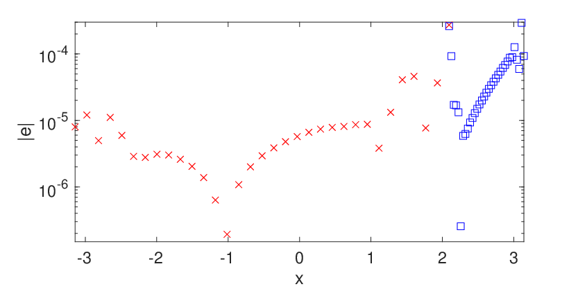
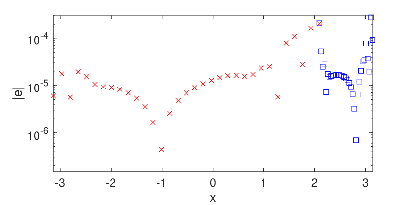
For time discretization we apply the classical fourth order explicit Runge-Kutta scheme with a time step size given by . To illustrate the fact that discrete geometric conservation is not necessary, we use the exact values of in the scheme (41) rather than solving the coupled system (52) in time. For comparison, we also consider the stationary domain case , in (56) using the same block grid as in the moving domain case at , as well as the same manufactured exact solution. The resulting absolute error levels at are plotted in Figure 2 using grid spacings in the boundary layer grid. In Table 1 we also compare the convergence rates between the moving and stationary domain cases. The convergence rate is close to three in both cases, with small differences in absolute error levels. The result of this experiment thus indicates that the proposed method-of-lines approach is comparable in terms of numerical efficiency between a moving domain and the equivalent stationary domain application.
 |
 |
 |
 |
| stationary | moving | ||||||
|---|---|---|---|---|---|---|---|
| 8 | -1.8639 | - | -2.0192 | - | |||
| 16 | -2.6741 | 2.69 | -2.7303 | 2.36 | |||
| 32 | -3.5329 | 2.85 | -3.5558 | 2.74 | |||
| 64 | -4.3916 | 2.85 | -4.4243 | 2.89 | |||
| 128 | -5.2678 | 2.91 | -5.3045 | 2.92 | |||
6 Conclusions
We have developed a framework based on semi-bounded operators for analyzing and discretizing initial boundary value problems on domains and meshes subject to arbitrary motion. This framework can be used to both analyze the linear well-posedness of the continuous problem as well as to formulate energy stable semi-discretizations. In particular, we have demonstrated that any energy estimate derived with respect to the physical coordinate system is associated with a semi-bounded property on the stationary reference domain. Since, with the right set-up, the main continuous result could be proven based on integration-by-parts only, the semi-discrete framework could be developed at a high level of abstraction based on discrete summation-by-parts, and thus valid for many different types of numerical discretization methods.
As a result of this development, initial boundary value problems posed on moving domains can be discretized in space and time separately in a stable way, i.e. using a standard method-of-lines approach. This does not require that discrete geometric conservation (free-stream preservation) holds for the combined spatial and temporal discretization. As a final bonus we also demonstrated that free-stream preservation can be achieved if so desired, both on the semi-discrete level as well as for fully discrete solutions. However, we stress that this is not strictly necessary for either high order accuracy or stability. The stability and efficiency of the new method-of-lines framework, even in the absence of discrete geometric conservation, was corroborated through a numerical experiment.
Appendix A Curvilinear coordinates
Here we discuss in more detail the special case where the moving domain coordinates for each time are expressed by a smooth bijective mapping from the unit hypercube . Provided that a discrete quadrature rule is available for , we can then always define a corresponding quadrature for as before using , where contains nodal values of the Jacobian determinant, either exact or approximated.
Note that any specific choice of simultaneously dictates the value of by the relation (37). For example, in D we have the exact expression
and it is therefore natural to either insert these continuous values in directly, or alternatively to apply discrete partial derivative operators on in order to define
| (58) |
With this choice, the discrete variable becomes
| (59) | ||||
where on the right hand side we have inserted the time derivative of the right hand side in (58).
Conversely, we always have the option to first specify the value of , for example by applying a set of physical space SBP operators as in (50), and then use the relation (37) constructively in order to define .
A.1 Free-stream preservation
Again using the example of D coordinates for brevity, SBP operators with respect to the physical coordinates in can be defined as follows, only provided that and are SBP operators (30) with respect to the reference domain quadrature ,
see also [24, 1] for more details. Now assume that and are consistent, i.e.
and assume furthermore that and commute, i.e. . Notably, this commuting property is automatically satisfied if the operators have a tensor (Kronecker) product structure, i.e. , . From these two assumptions of consistency and commutativity, we can write
i..e. the consistency assumption (51) used in Lemma 13 is satisfied. However, condition (50) of the same lemma clearly leads to a different value of than the one in (59). Hence the approximation (58) is not suitable if free-stream preservation is desirable (the same conclusion of course also applies if the exact values of are used). Instead we must take as given from (50), and then make constructive use of the initial value problem (37) in order to define . According to proposition 13, this leads to semi-discrete free-stream preservation. Also recall that, for fully discrete free-stream preservation we need to solve the semi-coupled system (52) for both and simultaneously by applying the same time integration scheme to both equations.
Acknowledgments
This work is based on research supported in part by the National Research Foundation of South Africa (Grant Numbers: 89916). Tomas Lundquist was also partly funded through Vetenskapsrådet, Sweden grant agreement 2020-03642 VR and the Swedish e-Science Research Centre (SeRC). Jan Nordström was supported by Vetenskapsrådet, Sweden grant 2018-05084 VR and SeRC. The opinions, findings and conclusions or recommendations expressed is that of the authors alone, and the NRF accepts no liability whatsoever in this regard.
References
- [1] O. Ålund and J. Nordström, Encapsulated high order difference operators on curvilinear non-conforming grids, Journal of Computational Physics 385 (2019), 209 – 224.
- [2] Douglas N. Arnold, Franco Brezzi, Bernardo Cockburn, and L. Donatella Marini, Unified analysis of discontinuous Galerkin methods for elliptic problems, SIAM Journal on Numerical Analysis 39 (2002), no. 5, 1749–1779.
- [3] Santiago Badia and Ramon Codina, Analysis of a stabilized finite element approximation of the transient convection‐diffusion equation using an ALE framework, SIAM Journal on Numerical Analysis 44 (2006), no. 5, 2159–2197.
- [4] Ted Belytschko, Wing Kam Liu, and Brian Moran, Nonlinear finite elements for continua and structures, John Wiley & Sons, Ltd, 2000 (English).
- [5] Daniele Boffi and Lucia Gastaldi, Stability and geometric conservation laws for ALE formulations, Computer Methods in Applied Mechanics and Engineering 193 (2004), no. 42, 4717–4739.
- [6] Andrea Bonito, Irene Kyza, and Ricardo H. Nochetto, Time-discrete higher order ALE formulations: a priori error analysis, Numerische Mathematik 125 (2013), no. 2, 225–257.
- [7] , Time-discrete higher-order ALE formulations: Stability, SIAM Journal on Numerical Analysis 51 (2013), no. 1, 577–604.
- [8] M. Carpenter and D. Gottlieb, Spectral methods on arbitrary grids, Journal of Computational Physics 129 (1996), 74–86.
- [9] M. H. Carpenter, D. Gottlieb, and S. Abarbanel, Time-stable boundary conditions for finite-difference schemes solving hyperbolic systems: Methodology and application to high-order compact schemes, Journal of Computational Physics 111 (1994), no. 2, 220–236.
- [10] S. Étienne, A. Garon, and D. Pelletier, Perspective on the geometric conservation law and finite element methods for ALE simulations of incompressible flow, Journal of Computational Physics 228 (2009), no. 7, 2313–2333.
- [11] Charbel Farhat, Philippe Geuzaine, and Céline Grandmont, The discrete geometric conservation law and the nonlinear stability of ALE schemes for the solution of flow problems on moving grids, Journal of Computational Physics 174 (2001), no. 2, 669–694.
- [12] Luca Formaggia and Fabio Nobile, A stability analysis for the arbitrary Lagrangian Eulerian formulation with finite elements, East-West Journal of Numerical Mathematics 7 (1999).
- [13] Luca Formaggia and Fabio Nobile, Stability analysis of second-order time accurate schemes for ALE–FEM, Computer Methods in Applied Mechanics and Engineering 193 (2004), no. 39, 4097–4116.
- [14] G. J. Gassner, A skew-symmetric discontinuous galerkin spectral element discretization and its relation to SBP-SAT finite difference methods, SIAM Journal of Scientific Computing 35 (2013), 1233–1253.
- [15] Sigal Gottlieb, On high order strong stability preserving Runge–Kutta and multi–step time discretizations, J. Sci. Comput. 25 (2005), 105–128.
- [16] M.E. Gurtin, An introduction to continuum mechanics, Academic Press, 1981.
- [17] B. Gustafsson, High order difference methods for time dependent pde, Springer-Verlag, 2008.
- [18] J. E. Hicken and D. W. Zingg, Summation-by-parts operators and high order quadrature, Journal of Computational and Applied Mathematics 237 (2013), no. 1, 111–125.
- [19] David A. Kopriva, Andrew R. Winters, Marvin Bohm, and Gregor J. Gassner, A provably stable discontinuous Galerkin spectral element approximation for moving hexahedral meshes, Computers & Fluids 139 (2016), 148–160.
- [20] Heinz-Otto Kreiss and Jens Lorenz, Initial-boundary value problems and the Navier-Stokes equations, Society for Industrial and Applied Mathematics, 2004.
- [21] L. Gary Leal, Advanced transport phenomena: Fluid mechanics and convective transport processes, Cambridge Series in Chemical Engineering, Cambridge University Press, 2007.
- [22] Doron Levy and Eitan Tadmor, From semidiscrete to fully discrete: Stability of Runge–Kutta schemes by the energy method, SIAM Review 40 (1998), no. 1, 40–73.
- [23] Viktor Linders, Tomas Lundquist, and Jan Nordström, On the order of accuracy of finite difference operators on diagonal norm based summation-by-parts form, SIAM Journal on Numerical Analysis 56 (2018), 1048 – 1063.
- [24] T. Lundquist, A. Malan, and J. Nordström, A hybrid framework for coupling arbitrary summation-by-parts schemes on general meshes, Journal of Computational Physics 362 (2018), 49–68.
- [25] , Efficient and error minimized coupling procedures for unstructured and moving meshes, Journal of Computational Physics 406 (2020), 109158.
- [26] T. Lundquist and J. Nordström, Stable and accurate filtering procedures, Journal of Scientific Computing 82 (2020), no. 16.
- [27] Tomas Lundquist, Fredrik Laurén, and Jan Nordström, A multi-domain summation-by-parts formulation for complex geometries, Journal of Computational Physics 463 (2022), 111269.
- [28] Cesar A. Acosta Minoli and David A. Kopriva, Discontinuous Galerkin spectral element approximations on moving meshes, Journal of Computational Physics 230 (2011), no. 5, 1876–1902.
- [29] S. Nikkar and J. Nordström, Fully discrete energy stable high order finite difference methods for hyperbolic problems in deforming domains, Journal of Computational Physics 291 (2015), 82 – 98.
- [30] J. Nordström, Conservative finite difference formulations, variable coefficients, energy estimates and artificial dissipation, Journal of Scientific Computing 29 (2006), no. 3, 375–404.
- [31] J. Nordström and M. H. Carpenter, High-order finite difference methods, multidimensional linear problems and curvilinear coordinates, Journal of Computational Physics 173 (2001), 149–174.
- [32] J. Nordström, K. Forsberg, C. Adamsson, and P. Eliasson, Finite volume methods, unstructured meshes and strict stability for hyperbolic problems, Applied Numerical Mathematics 45 (2003), 453–473.
- [33] Jan Nordström, A roadmap to well posed and stable problems in computational physics, Journal of Scientific Computing 71 (2017), no. 1, 365–385.
- [34] Jan Nordström and Thomas M. Hagstrom, The number of boundary conditions for initial boundary value problems, SIAM Journal on Numerical Analysis 58 (2020), no. 5, 2818–2828.
- [35] P.-O. Persson, J. Bonet, and J. Peraire, Discontinuous Galerkin solution of the Navier–Stokes equations on deformable domains, Computer Methods in Applied Mechanics and Engineering 198 (2009), no. 17, 1585–1595.
- [36] Hendrik Ranocha and Philipp Öffner, L2 stability of explicit Runge–Kutta schemes, Journal of Scientific Computing 75 (2018), no. 2, 1040–1056.
- [37] Chi-Wang Shu, Total-variation-diminishing time discretizations, SIAM Journal on Scientific and Statistical Computing 9 (1988), no. 6, 1073–1084.
- [38] Zheng Sun and Chi-Wang Shu, Strong stability of explicit Runge–Kutta time discretizations, SIAM Journal on Numerical Analysis 57 (2019), no. 3, 1158–1182.
- [39] Zhou, Lingling, Xia, Yinhua, and Shu, Chi-Wang, Stability analysis and error estimates of arbitrary Lagrangian-Eulerian discontinuous Galerkin method coupled with Runge-Kutta time-marching for linear conservation laws, ESAIM: M2AN 53 (2019), no. 1, 105–144.