Learning from Noisy Crowd Labels with Logics Thanks: *Corresponding author.
Abstract
This paper explores the integration of symbolic logic knowledge into deep neural networks for learning from noisy crowd labels. We introduce Logic-guided Learning from Noisy Crowd Labels (Logic-LNCL), an EM-alike iterative logic knowledge distillation framework that learns from both noisy labeled data and logic rules of interest. Unlike traditional EM methods, our framework contains a “pseudo-E-step” that distills from the logic rules a new type of learning target, which is then used in the “pseudo-M-step” for training the classifier. Extensive evaluations on two real-world datasets for text sentiment classification and named entity recognition demonstrate that the proposed framework improves the state-of-the-art and provides a new solution to learning from noisy crowd labels.
Index Terms:
crowdsourcing, noisy labels, weak supervision, neural-symbolic learningI Introduction

Deep learning heavily relies on the size and quality of labeled training data. Crowdsourced data annotation offers a time- and cost-efficient means to collect large-scale datasets for deep learning tasks [1]. However, due to the imperfect crowd annotators, crowdsourced labels are often noisy; this has become a key concern for training deep neural networks [2].
To learn a classifier in the context of noisy crowd labels, existing methods fall into two paradigms, as shown in Figure 1: (1) The two-stage learning-from-noisy-crowds-labels (LNCL) paradigm that first uses truth inference methods [3, 4, 5, 6, 7, 8, 9, 10, 11] to infer the true label of each instance and then performs traditional supervised learning; (2) The one-stage LNCL paradigm that directly learns from noisy crowds labels in an end-to-end manner using ad hoc LNCL methods [12, 13, 14, 15, 16, 17, 18, 19, 20, 21], which use all available information together to perform global optimization to obtain the classifier of interest and generally result in better performance. Specifically, existing work on the recently prevailing one-stage LNCL mainly take two approaches: probabilistic or deep learning. The probabilistic approach models true labels as latent variables and uses expectation maximization (EM) to infer the true labels and to learn the parameters of the classifier (which generally be a deep neural network) in an iterative manner [12, 13, 14, 15, 16]. More recent efforts have focused on the deep learning approach, which trains a deep neural architecture from noisy labels in an end-to-end manner, by introducing into the architecture an extra neural layer that maps latent true labels to the noisy crowd labels [17, 19, 20, 21].
In the broader AI community, there is a well-known thorny problem for all deep neural networks: while being flexible to capture complex mapping between the features and label, deep learning approaches are generally data-hungry and not robust—they only learn (possibly spurious) statistical correlations. In learning from noisy crowd labels, all existing prevailing one-stage LNCL approaches suffer much more from those issues for at least the following two reasons. (1) On the one hand, those approaches contain additional parameters that model the reliability of each individual crowd annotator; consequently, training those approaches—that contain parameters of both neural network classifiers and annotators—requires a much larger amount of data than the conventional neural networks; (2) On the other hand, the presence of label noise makes it harder for the neural network to recognize relevant information from the training data for classification. As a result, the learned data representations may turn out to be dominated by information irrelevant to the true labels, thus becoming useless or even negatively impacting the performance.
In comparison to learning-based, data-driven approaches, reasoning-based, knowledge-driven approaches are more sample-efficient and more robust because of their capability of representing concepts and the causal relations among them. Recent discussions in the AI communities have converged on the idea of integrating symbolic approaches with machine learning [22, 23]. A visible trend is the growing body of work on neural-symbolic methods. For example, Allamanis et al. [24] propose to learn continuous representations of symbolic knowledge for integration into neural networks; Xu et al. [25] present the semantic loss that augments the learning objective of neural networks with soft-constraints specified with domain knowledge. On the application side, neural-symbolic methods have been applied to both vision and language tasks including visual relation prediction [26], visual question answering (VQA) [27], text sentiment analysis [28], and semantic parsing [29].
In this paper, we move one step further and explore: in the presence of noisy crowd labels that makes the model more vulnerable and data-hungry, how can we capitalize on the interpretable and robust logic knowledge in learning from noisy crowd labels to improve the model’s generalization? Despite the obvious benefit of the neural-symbolic paradigm, it remains unclear how to best exploit logic knowledge in our context—existing neural-symbolic methods are not easily applicable due to the specific need for the inference of true labels from noisy crowd labels. Specifically, properly inferring true labels needs to take into account the influence of logic knowledge and the reliability of annotators, while learning the parameters of the classifiers in a unified and principled framework. To address these problem, we introduce Logic-guided Learning from Noisy Crowd Labels (Logic-LNCL), an EM-alike iterative logic knowledge distillation framework that allows neural networks to learn simultaneously from the noisy labels and logic rules. Unlike all existing probabilistic models for learning from crowd labels, in our “pseudo-E-step”, we introduce a new type of learning target by adapting the original learning target with posterior regularization defined by the rules. Then, inspired by knowledge distillation [30], both the original and adapted learning targets are used in the “pseudo-M-step” to update the parameters of the deep neural networks and those of the crowd annotators. By doing so, our framework seamlessly integrates symbolic logic knowledge and the inference for true labels, while allowing the deep neural network to learn from both data and logic knowledge.
Contributions. To the best of our knowledge, this is the first work to incorporate logic rules in learning from noisy (crowd) labels problems with a principled framework. We introduce Logic-LNCL, an EM-alike iterative logic knowledge distillation framework for learning from both noisy crowd labels and logic rules. We demonstrate the versatility of Logic-LNCL by instantiating it on two representative language tasks, text sentiment classification and named entity recognition. We conduct extensive evaluations of our proposed framework on real-world datasets, showing that Logic-LNCL improves the classifier’s generalization and outperforms the state-of-the-art.
II Preliminaries
II-A Problem Formulation: Learning from Noisy Crowd Data
Let be an i.i.d. dataset. For each instance , we have a vector of noisy labels given by a total of annotators, where represents the label by the annotator on instance . Each instance has its corresponding unobserved, latent ground truth , where represents the number of categories. In addition, considering that for each instance, often not every annotator has annotated it, we use to denote that annotator has not annotated instance . Our main goal is to train an accurate classifier for predicting given new unknown instances by using noisy training data .
II-B Prior Art Utilized by Us
Our framework builds on a canonical probabilistic graphical model [12, 15] as a principled cornerstone. Here we introduce the basic model, whose graphical representation is shown in Figure 2.
In this latent variable model, first, for each instance ,
| (1) |
where the distribution of its unobserved ground truth comes from a conditional categorical distribution ; is a flexible neural network model parametrized by . Note that the classifier in the original work [12] is a logistic regression. Then, the reliability of the annotator is modeled by an annotator-specific confusion matrix , representing the likelihood of the annotator on identifying the ground truth label as any (other) labels. Formally, given and , the distribution of crowd label is determined by:
| (2) |
where . Based on the model construction, the optimization objective is to maximize the log conditional likelihood of the observed crowd labels given instance features, i.e., , with respect to the parameters . Those parameters can be learned by the EM algorithm.
III Method
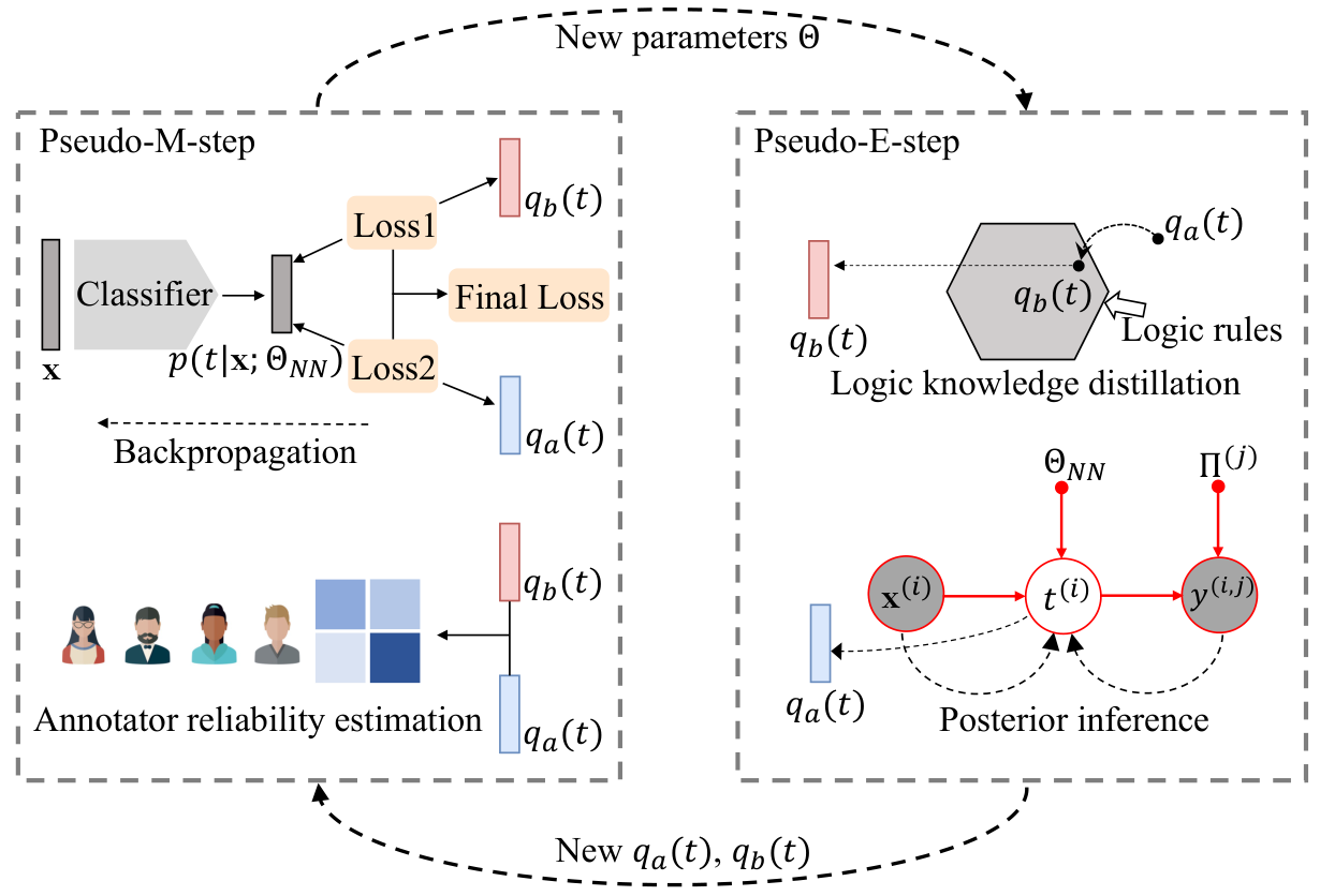
This section introduces our proposed framework Logic-LNCL depicted in Figure 3. We start by introducing the additional “learning resources”, i.e. logic rules, in addition to the noisy labeled data mentioned in the Section II-A. Then we present the proposed EM-alike iterative learning algorithm.
III-A Logic Rules
Input:
Data ;
Rule set
;
Parameter : imitation strength;
Parameter : regularization strength
Output:
We introduce the off-the-shelf theory of probabilistic soft logic (PSL) [31] to encode first-order logic rules. Under the theory of PSL, we consider a set of first-order logic rules with weights, i.e., , where is the -th rule, and represents the degree of credibility or importance. When all the variables in a logic rule are instantiated, it forms a “grounding”; and when the rules we defined are applied to data instances, a set of groundings of , denoted as , are formed. refers to the total number of groundings instantiated in the dataset for the -th rule. To illustrate rules in PSL, the following example encodes the voting behavior of two voters:
| (3) |
where , and are called “atoms” (denoted as ), and their soft truth values take value space of instead of the extremes and only. PSL uses the following relaxation of the logical conjunction (), disjunction (), and negation () for logic operators:
| (4) | ||||
where obtains the soft truth values. In the above example, after instantiating and and , we have .
As a remark, the logic rules introduced in our Logic-LNCL framework can be any first-order soft logic rules that follow the PSL formalism. Our framework is not compatible with other types of logic, such as the high-order logic.
III-B Pseudo-M-step: Learning
In the Pseudo-M-step, we aim to use two learning targets to learn the parameters of the classifier and the annotators: the learning target from the conventional EM algorithm and a second target that contains the distilled logic knowledge.
Based on the probabilistic model and optimization objective constructed in Section II-B, the M-step in the conventional EM algorithm updates the parameters of the neural network by maximizing11 1 Derivation of the solution is given in Section V-A.:
| (5) |
or:
| (6) |
where is the ground truth estimation obtained from the previous E-step, weight is the number of annotators annotated . Equation 6 comes from the strict derivation of the EM algorithm, and Equation 5 comes from our adaptation of Equation 6 with the addition of weight . The reason for considering the new objective function of Equation 5 is that the instances with more annotations are likely to have more accurate posterior distribution. Both of these objectives allow the neural network to mimic the ground truth estimation , and we have the flexibility to choose one of the objectives in our experiments. In the following derivation, we assume that we adopt Equation 6 for simplicity.
We did not straight follow Equation 6 to optimize the classifier parameters. Instead, inspired by knowledge distillation [30], we introduce logic rules into the learning procedure by considering an extra learning target from logic knowledge distillation, denoted as , in additional to the original learning target (Equation 6), denoted as . As shown in Figure 3, the loss function in our Pseudo-M-step is then formulated by:
| (7) | |||
where is the imitation hyper-parameter balancing between the two parts; denotes the cross-entropy loss function. For the setting of here, we can set it as a constant or a variable that constantly changes during the training progress. The process of the neural network imitating essentially transfers the logic knowledge into the neural network. Note that both the target and will be updated in the Pseudo-E-step. Considering the equivalence of negative log-likelihood and cross-entropy loss, and the loss function in Equation 7 is linear with respect to the label , the final loss function can be written as:
| (8) |
where
| (9) |
The weighted version of Loss can be easily obtained as:
| (10) |
When we use standard mini-bath gradient descent to optimize the Loss in Equation 8 (or Equation 10), the parameters will be updated:
| (11) |
where is learning rate, and are mini-batch data and batch size, respectively.
Both the original knowledge distillation method [30]22 2 Hinton et al. [30] found that a classifier can be better trained using the predictions of another well-trained classifier as the learning target together with the original training labels, compared to using the original labels only. Calling the procedure knowledge distillation, they found there is a positive effect even when the classifier for providing help (called teacher) is pre-trained with the same data as those later used for training the target classifier (called student). and our framework forces the neural network (i.e., ) to imitate an additional distilled knowledge target in addition to a basic target. The major difference lies in that, the goal of Hinton et al. [30] is to better train a “student” neural network from another “teacher” neural network with better generalization ability, while our goal is to enable the neural network to learn from the knowledge distilled from logic rules of interest; another technical difference is that, while the two learning targets in Hinton et al. [30] are fixed, our two targets and model parameters are continuous iteratively updated during the EM-alike procedure.
We now proceed to updating the parameters of the crowd annotators . Analogous to optimizing the neural network parameters, we can optimize crowd annotators’ parameters according to the probabilistic model constructed in Section II-B and follow the EM’s general recipe to directly obtain their closed-form solutions. Here, we once again use as the final ground truth estimation to replace the original , and obtain33 3 Derivation of the solution is given in Section V-A.:
| (12) |
where means the annotator labeled the instance ; and is an indicator function that takes the value when the internal declaration is true, and otherwise.
III-C Pseudo-E-step: Inference
III-C1 Target Construction
Here, we assume that the variables of interest strictly obey the basic probabilistic graphical model (Figure 2). The posterior distribution of the latent variable , , is inferred using the Bayes’ theorem:
| (13) | |||
where represents all the annotators who annotated the instance; the parameters are from the previous Pseudo-M-step.
III-C2 Target Construction
We aim to construct such that it fits the pre-defined logic rules while making being as close to as possible. To do so, we project into a rule-regularized subspace using posterior regularization [32, 28].
We first use an expectation operator to impose the rule constraints on : , where is the rule’s value of 44 4 corresponds to in probabilistic soft logic (PSL) formalism [33], where is called as “distance to satisfaction” in PSL; when a rule is fully satisfied, then . . That is, we expect the distribution of in the grounded instance to conform to the logic rule. In the meanwhile, to keep close to , we minimize the KL-divergence between those distributions. This leads to following optimization problem:
| (14) |
where is the regularization parameter; denotes the slack variable of the respective logic constraint. This optimization problem, which is convex, can be solved through its dual form and obtain the closed-form solutions55 5 Derivation of the solution is given in Section V-B.:
| (15) |
Intuitively, will be greater for the cases when the corresponding rule is satisfied, thus increasing , and vice versa. From more intuitive perspective, the part embedded with logic knowledge plays the role of a “constraint function”, or “reward function”.
The overall learning procedure is summarized in Algorithm 1. We note that unlike all previous LNCL models, the proposed Logic-LNCL seamlessly integrates the following four processes—all necessary for allowing the classifier to learn simultaneously from noisy crowd labels and logic rules—in a principled EM-alike iterative logic knowledge distillation framework. These processes are: (i) inference of latent ground truth; (ii) logic knowledge distillation attached to latent ground truth using posterior regularization; drawn on the knowledge distillation idea, (iii) learning of classifier parameters, and (iv) learning of annotator reliability.
Implementation details: employ at test phase. For instances without crowd labels at the test phase, we can employ either the trained neural network for prediction, i.e., , or taking a step further, adapt this prediction using Equation 15 to account for the logic rule. To do so, we simply need to replace by in Equation 15.
IV Applications
We instantiate our framework on two representative language tasks, text sentiment classification and named entity recognition (NER). This section introduces the logic rules considered for integration. Note that since NER is a typical class of sequence labeling tasks, it is also easy to extend the proposed framework to other parallel tasks, such as part-of-speech (POS) tagging.
IV-A Sentiment Classification
In sentiment analysis, identifying contrastive sense in the sentence to capture the dominant sentiment precisely is a challenge for the classifier. For humans, a useful clue of such contrastive sense is the widely-used conjunction word “but”, which is a vital sign for sentiment change within a sentence. For those sentences containing “but”, the sentiment of clauses after “but” generally dominates. Considering that a sentence S has an “A-but-B” structure; we would expect the sentiment inclination of the entire sentence is consistent with the sentiment inclination of the clause B. Formally, this can be expressed with the logic rule:
| (16) |
| (17) |
where and denotes the probability of clause for “positive and “negative”. We set the weight of both rules to . Thus, we can get that the rule’s value takes when and otherwise.
IV-B Named Entity Recognition
For NER, the basic network largely ignore the constraint that should exist between valid consecutive labels. For instance, the labels before the “I-ORG” (“Inside-Organization”) can only be “B-ORG” (“Begin-Organization”) or “I-ORG” (“Inside-Organization”) but not “B-PER” (“Begin-Person”) etc. Unlike recent work [34] that adds a conditional random field (CRF) to model bi-gram dependencies within label seqence, we apply the logic rules without introducing additional parameters that need to be learned. Two example rules are:
| (18) |
| (19) |
The bi-gram dependencies are introduced by the logic rules that express the transition relationship which should exist within true labels. With the theory of probabilistic soft logic and the weights of the rules (e.g., and , which can be set through human knowledge, lightweight sample statistics, etc.), the weighted values of rules in Equations 18 and 19 can take and , respectively. According to the transition rules, we can use dynamic programming for efficient computation in Equation 15.
V Proofs
This section provides two necessary proofs to support some of the conclusions in Section III. Section V-A introduces parameter estimation of the basic graph model (to support Equations 6, 12, and 13), and Section V-B introduces the derivation process for solving the optimization problem in Equation 14 (to support Equation 15).
V-A Proof: Parameter Estimation of The Basic Graph Model
For the basic graph model constructed in Section II-B, the log-likelihood can be written as:
| (A.1) | ||||
The last step of this derivation which obtains the (called “Evidence Lower Bound (ELBO)”) used Jensen’s inequality [35]; for each , can be some distribution over the . Note that we use to denote in Section III and blow derivation for simplicity.
We then proceed to apply the general EM recipe to perform iterative calculations to solve the optimization problem:
| (A.2) | ||||
| (A.3) | ||||
where . During the E-step, the posterior is obtained by using of Bayes’s theorem given the parameters learned on the last M-step. During the M-step, we can easily obtain the optimization objective in Equation 6 according to Equation A.3, and we can obtain the closed-form solution of by equating the gradient of Equation A.3 to zero.
V-B Proof: Solving the Optimization Problem in Equation 14
Here we provide the derivation process for solving the optimization problem in Equation 14 to obtain the solution in Equation 15. The optimization problem is:
| (B.1) |
Here note that we assume that for instance , each rule can act on it and form a grounding.
The following proofs are largely adapted from Ganchev et al. [36] and Hu et al. [28]. The Lagrangian of Equation B.1 is:
| (B.2) |
where:
| (B.3) |
Given Equation B.2, we can obtain:
| (B.4) |
| (B.5) | |||
| (B.6) |
For simplicity, let , , . Plugging Equation B.6 into Equation B.4, we obtain:
| (B.7) | ||||
| (B.8) |
Plugging Equation B.8 into , we obtain:
| (B.9) | ||||
We have because of Equation B.5, and since monotonically decreases when increases, therefore:
| (B.10) | ||||
Plugging Equation B.6 and Equation B.10 into Equation B.4, we obtain the final solution of as in Equation 15.
VI Evaluation
VI-A Setup
VI-A1 Datasets
We evaluate our framework on sentiment classification and named entity recognition using two real-world public datasets66 6 Code and datasets are available from https://github.com/junchenzhi/Logic-LNCL.: the Sentiment Polarity (MTurk) dataset [13] (balanced categories), and the CoNLL-2003 NER (MTurk) dataset [14]. Crowd labels in both datasets were contributed by annotators from Amazon Mechanical Turk (MTurk).
Sentiment Polarity (MTurk) Dataset. This crowdsourced dataset [13] is constructed from the well-established sentence-level sentiment polarity dataset [37] with crowd labels. The dataset contains sentences from movie reviews extracted from the website RottenTomatoes.com and the sentiment was classified as positive or negative. The training data contains sentences, crowd labels annotated by different annotators. The test data contains sentences, which we shuffled and divided into a development set and a test set containing 3000 samples and 2789 samples, respectively.
CoNLL-2003 NER (MTurk) Dataset. This crowdsourced dataset [14] is constructed from the well-established CoNLL-2003 NER dataset [38] with crowd labels. The goal is to recognize named entities (person, location, organization, miscellaneous) together with their different parts (begin, inside) in the sentence. All categories include: B-PER, I-PER, B-LOC, I-LOC, B-ORG, I-ORG, B-MISC, I-MISC, Others. The training set contains sentences annotated by different annotators, whose F1 scores against the ground truth vary from to . We shuffled and divided the test samples [14] into a development set and a test set containing 2000 samples and 1250 samples, respectively. It is worth mentioning that, crowd labels in the NER dataset may contain three main types of errors that annotators make during the annotation process: (i) Ignore error: entity is not annotated by the annotator; (ii) Boundary error: entity type is correctly identified, but the annotated span does not match exactly; and (iii) Span type error: the entity type within the annotation span is wrong.
VI-A2 Compared methods
We consider the following representative LNCL (learning-from-noisy-crowds-labels) competitors: (i) MV-Classifier, a two-phase method that first estimates the ground truth from noisy labels by MV (Majority Voting), and then trains the classifier; (ii) GLAD-Classifier, similar to MV+Classifier, except the ground truth is estimated by GLAD [4]; (iii) Raykar [12] and AggNet [13], two representative probabilistic models described in Section II-B; (iv) Three variants of the state-of-the-art method CL [17] for deep learning from crowd labels: CL (MW), CL (VW), and CL (VW-B), where “MW”, “VW” and “VW-B” refer to three different ways of parameterizing annotator reliability; (v) DL-DN∗ and DL-WDN∗ [18], which trains an individual network from the labels of each crowd annotator and aggregates the output from all networks for prediction; (vi) Our proposed variants Logic-LNCL-student and Logic-LNCL-teacher using , and , as the output (details in paragraph “Implementation details: employ at test phase”), respectively; Finally, we consider (vii) Gold, denoting the classifier trained in the ideal case when true labels are known.
In addition, we analyze the inference performance of the truth inference methods on the training set. (1) On the sentiment polarity dataset, we consider the baseline MV, the two state-of-the-art graph models DS [3] and GLAD [4], and heuristic iterative inference based PM [10] and CATD [11]; (2) On the NER dataset, we consider the baseline MV, two NER-oriented extended graph models DS [3] and IBCC [7] (which were originally designed for the traditional classification task), and ad hoc NER-oriented graph models BSC-seq [8] and HMM-Crowd [39].
VI-A3 Configurations
| Sentiment Dataset | NER Dataset | ||
|---|---|---|---|
| Hyper-parameters | Imitation strength (: epoch) | ||
| Regularization strength | |||
| Early stopping patience | |||
| Optimizer | Adadelta† | Adam§ | |
| Learning rate | + weight decay∗ | § | |
| Epoch | † | § | |
| Batch size | 50† | 64§ | |
| Network architecture | Follow† | Follow§ | |
| Data division (train/development/test) | 4999/3000/2789 | 5985/2000/1250 | |
| Resource | NVIDIA Tesla V100 32GB GPUs | ||
- 1
†: The network architecture and hyper-parameters are fully consistent with Kim [40].
- 2
§: The network architecture and hyper-parameters are fully consistent with Rodrigues and Pereira [17].
- 3
∗: For all methods on the sentiment dataset, we added weight decay for original learning rate in Kim [40], i.e., decay by half every epochs, to obtain more stable results.

| Paradigm | Method | Prediction | Inference† | Average |
|---|---|---|---|---|
| Two-stage LNCL | MV-Classifier | 78.08 | 88.58 | 83.33 |
| GLAD-Classifier | 78.45 | 91.76 | 85.11 | |
| One-stage LNCL | Raykar [12] | - | 91.48 | - |
| AggNet [15] | 78.47 | 91.63 | 85.05 | |
| CL (VW) [17] | 78.22 | 88.00 | 83.11 | |
| CL (VW-B) [17] | 78.04 | 87.51 | 82.78 | |
| CL (MW) [17] | 78.28 | 88.30 | 83.29 | |
| Logic-LNCL-student | 78.85 | 91.82 | 85.34 | |
| Logic-LNCL-teacher | 79.22 | 91.82 | 85.52 | |
| Truth Inference | MV | - | 88.58 | - |
| DS [3] | - | 91.48 | - | |
| GLAD [4] | - | 91.76 | - | |
| PM [10] | - | 89.66 | - | |
| CATD [11] | - | 91.49 | - | |
| - | Gold | 79.26 | 100 | 86.13 |
- 1
†: Inference† denotes inference accuracy on the training set (results inferred by MV and GLAD; truth posterior estimation in AggNet; the classifiers’ outputs in CLs; in Logic-LNCLs).
| Prediction | Inference† | |||||||
| Paradigm | Method | Precision | Recall | F1 | Precision | Recall | F1 | Avg. F1 |
| Two-stage LNCL | MV-Classifier | 65.14 | 45.98 | 53.89 | 79.12 | 58.50 | 67.27 | 60.58 |
| One-stage LNCL | AggNet [15] | 61.67 | 58.64 | 60.09 | 77.19 | 73.02 | 75.04 | 67.57 |
| CL (VW, 5§) [17] | 69.37 | 52.11 | 59.32 | 79.19 | 71.72 | 75.25 | 67.29 | |
| CL (VW-B, 5§) [17] | 58.23 | 59.92 | 58.97 | 75.27 | 73.41 | 74.30 | 66.64 | |
| CL (MW, 5§) [17] | 62.98 | 61.57 | 62.19 | 78.37 | 75.14 | 76.70 | 69.45 | |
| CL (MW, 1§) [17] | 53.75 | 44.70 | 48.19 | 61.93 | 50.21 | 54.42 | 51.31 | |
| Logic-LNCL-student | 66.53 | 59.29 | 62.69 | 84.90 | 74.11 | 79.14 | 70.92 | |
| Logic-LNCL-teacher | 70.10 | 58.99 | 64.06 | 84.90 | 74.11 | 79.14 | 71.60 | |
| CRF-MA∗ [14] | 49.4 | 85.6 | 62.6 | 86.0 | 65.6 | 74.4 | 68.50 | |
| DL-DN‡ [18] | 72.3 | 45.9 | 56.2 | - | - | - | - | |
| DL-WDN‡ [18] | 61.1 | 48.0 | 53.4 | - | - | - | - | |
| Truth Inference | MV | - | - | - | 79.12 | 58.50 | 67.27 | - |
| DS [3]⋆ | - | - | - | 79.0 | 70.4 | 74.4 | - | |
| IBCC [7]⋆ | - | - | - | 79.0 | 70.4 | 74.4 | - | |
| BSC-seq [8]∗ | - | - | - | 80.3 | 74.8 | 77.4 | - | |
| HMM-Crowd [9]∗ | - | - | - | 77.40 | 72.29 | 74.76 | - | |
| - | Gold (Upper Bound) | 72.52 | 73.51 | 72.98 | 100 | 100 | 100 | 86.49 |
- 1
†: Inference† refers to the meaning similar to the one in Table II.
- 2
§: and denote the number of times the classifier is pre-trained using the labels estimated from MV.
- 3
∗: results are reported from the original work.
- 4
We show the configurations in Table I. For the two datasets, the neural network configurations in our proposed methods and the compared methods remain consistent with Kim [40] and Rodrigues and Pereira [17], respectively. Refer to Figure 5 for more information about the networks. For the objective function in our pseudo-M-step, we use the Equation 6 and Equation 5 on the two datasets, respectively. As presented in Section VI-A1 and on both datasets, we have separated a development set from the original test samples to tune the hyper-parameters and to determine the early stopping (epoch) time for all methods. Note that for the compared methods, there are no additional hyper-parameters.
VI-A4 Evaluation Metrics
VI-B Results and Analysis
The results on the two datasets are shown in Table II and Table III, respectively. In addition to the main results—the prediction performance and the inference performance of the LNCL methods—we also show the inference performance of the ad hoc truth inference methods on the training set. Here we first analyze the results of the most interest, i.e., the model’s prediction performance. We observe that both proposed Logic-LNCL-student and Logic-LNCL-teacher outperform all the compared methods, indicating that our approach has a higher level of robustness to label noise. On the sentiment polarity dataset, like the results reported in Atarashi et al. [16], most methods exhibit similarly high accuracy. This is mainly because a relatively more number of annotations were received for each instance (5.55 on average), rendering the inference for true labels a relatively easy task for all comparison methods. Further, we utilize the t-test (unilateral statistics) to check whether the differences between our methods and the most competitive AggNet are statistically significant. In the two metrics of prediction and inference, when comparing Logic-LNCL-student and AggNet, the t-values are /, and the p-values are both less than (i.e., statistically significant); when comparing Logic-LNCL-teacher and AggNet, the t-values are /, and the p-values are both less than .


| Sentiment Dataset | NER Dataset | ||||
|---|---|---|---|---|---|
| Method | Prediction | Inference | Prediction | Inference | Average |
| MV-Rule | 78.41 | 88.96 | 47.66 | 61.63 | 69.17 |
| GLAD-Rule | 78.62 | 91.74 | 61.65 | 77.52 | 77.38 |
| w/o-Rule | 78.47 | 91.63 | 60.11 | 75.28 | 76.37 |
| MV-t | 78.83 | 88.58 | 46.77 | 67.27 | 70.36 |
| our-other-rules-student | 78.79 | 91.72 | 50.71 | 75.07 | 74.07 |
| our-other-rules-teacher | 78.79 | 91.72 | 1.23 | 75.07 | 61.70 |
| Logic-LNCL-student | 78.85 | 91.82 | 62.69 | 79.14 | 78.13 |
| Logic-LNCL-teacher | 79.22 | 91.82 | 64.06 | 79.14 | 78.56 |
On the NER dataset, the performance of the compared methods shows a more considerable difference (Table III). Logic-LNCL-teacher and Logic-LNCL-student achieve the best and second-best performance on the F1 metric, respectively. Both variants of our framework surpass the compared methods with a large margin: they outperform the state-of-the-art AggNet by and , respectively, and vastly exceed the baseline MV-Classifier by and , respectively. An additional advantage of our methods compared to the competitive CL (MW) is that while CL (MW) relies on several epochs of pre-training on estimated labels with Majority Voting, our methods always learn from scratch without the need for additional pre-training on other methods.
Employing at test phase. Comparing the two variants of Logic-LNCL, we observe that Logic-LNCL-teacher outperforms the Logic-LNCL-student on both datasets, with a more significant margin on the NER dataset. These results demonstrate the utility of logic rules even in the test phase.
Inference performance. In addition to the above analysis of the generalization performance, we also observe in Table II and Table III that the Logic-LNCLs outperform all compared methods (containing the ad hoc truth inference methods) in terms of inference performance on the training set. Therefore, the logic knowledge distillation component in Logic-LNCLs can not only introduces “dark knowledge” [30] to the classifier to improve the generalization, but also can guide the ground truth inference process to directly improve inference accuracy so as to feed the classifier with better training information.
Advantage of sample-efficiency. Through further experiments, we find that on both datasets, both the student/teacher variants of our framework can achieve (and slightly exceed) the most competitive generalization performance in the compared methods (i.e., AggNet/CL(MW, 5)) using fewer training samples, i.e., / out of the original samples, / out of the original samples. Additionally, under these sample conditions, our variants student/teacher also generally obtain the best inference performance on the training data of the two datasets: /, /.
Annotator reliability estimation. We further analyze the estimation performance of annotator confusion matrices . Figures 6 and 7 show the high accuracy of the annotator confusion matrices estimated with Logic-LNCL. Such a result further demonstrates the effectiveness of our method. The way we obtained the four subfigures in Figures 6 and 7 is presented as follows. In Figure 6(a) and 7(a), similar to Rodrigues et al. [17], the six/four annotators with the largest number of labels were selected to analyze the confusion matrix estimation. We compare the estimated confusion matrices to the real ones, which are calculated based on their annotations and the ground truth. In Figure 6(b) and 7(b), for each annotator, we divide the sum of the diagonal values of the estimated matrix by and , respectively, to obtain a scalar to represent the overall reliability. Figure 6(b) shows all annotators except the anomalous annotators with five or fewer labels; Figure 7(b) shows all annotators.
Ablation study. We compare with an extensive array of possible variants of our framework. In Table IV, we observe: (i) Although MV-Rule and GLAD-Rule also distill knowledge from logic rules to provide the classifier to learn, they achieve suboptimal performance relative to Logic-LNCLs, mainly because they do not constantly refine the ground truth estimation during the iterative learning procedure like ours; (ii) On both datasets, our student model and teacher model outperform the important variant w/o-Rule. In particular, on the NER dataset, our models outperform w/o-Rule in prediction performance by and , respectively; (iii) The results of variants concerning relatively bad rules corroborate our intuition that rules that do not conform well to objective laws can not make the framework work satisfactorily; (iv) Our Logic-LNCLs surpasses all other competitors, demonstrating the superiority of seamlessly integrating the four essential processes in the principled iterative distillation framework: inference of ground truth, knowledge distillation from logic rules, learning of neural network and learning of annotator reliability; the interplay between these processes makes them mutually beneficial.
VII Related Work
Learning from noisy crowd labels has long been the goal of the weakly supervised learning community [41]. Back in early 1970s, Dawid and Skene [3] proposed a probabilistic graph model to inference the latent ground truth labels using the expectation maximization (EM) algorithm. This truth inference process is followed by a traditional supervised learning phase to complete the learning [42]. Since then, a variety of generalizations and improvements upon the original method have been proposed under the same probabilistic framework [4, 5, 43, 6, 44]. Another line of the research [12, 13, 15, 16, 17, 45, 20, 21] investigates learning directly from noisy crowdsourced labels without the preceding truth inference stage. To the best of our knowledge, our work is the first that considers the integration of symbolic logic knowledge for learning from noisy crowd labels.
Learning from noisy labels is a closely related, larger research area that concerns the presence of noisy labels, regardless of the sources of such labels. In this learning setting, the labels are not necessarily from crowds and often the case, there is only one noisy label for each instance. A large bulk of work has been proposed investigating different learning strategies, e.g., designing more robust loss function [46, 47], architecture [48, 49], regularization [50, 51], or a better way of selecting samples [52], etc. Essentially, many robust architecture-based methods in this learning setting [48, 49] are similar to those for learning from noisy crowd labels [12, 15, 17, 20]: they all infer the ground truth labels through a neural layer from the noisy labels.
VIII Discussion
We recently noticed that there had been related work [53] using LNCL methods to perform the similar weak supervision learning problem [53, 54], where annotation sources come from multiple programs defined artificially in advance instead of multiple crowd annotators. We plan to deploy our framework on weak supervision datasets in the future to demonstrate its versatility further. At a higher level, we advocate that for all learning tasks with ground truth latent variables (e.g., the extensively studied leaning-from-noisy-labels task presented in Section VII), the idea of Logic-LNCL can be transferable for iterative computation of learning and inference, where the inference process seamlessly combines the truth inference and logic knowledge distillation. Hence, we plan to extend our framework to the learning-from-noisy-labels task and conduct further empirical validation. For the limitations, one of the most noteworthy points we believe is that for vision tasks other than language tasks, it is more difficult to extend our framework yet. Because we need to propose a more complex unified framework containing the indispensable process of embedding continuous high-dimensional data into the semantic space to represent high-level concepts (used for logics).
IX Conclusion and Future Work
This paper proposes to incorporate symbolic logic knowledge into deep learning from noisy crowd labels. We introduce Logic-LNCL, an EM-alike iterative logic knowledge distillation framework that integrates logic knowledge with the inference for true labels, allowing the neural network to learn from both the logic knowledge and the data. Our method, therefore, benefits both from the flexibility of deep learning and the robustness of logic rules. Our experiments demonstrate that Logic-LNCL significantly improves base networks on sentiment classification and named entity recognition with logic rules. The encouraging results show a strong potential of our proposed framework for improving other learning tasks, such as vision tasks, which we plan to study in the future.
Acknowledgment
This work was supported by National Natural Science Foundation of China Under Grant Nos (61932007, 61972013, 62141209).
References
- [1] C. Chai, J. Fan, G. Li, J. Wang, and Y. Zheng, “Crowdsourcing database systems: Overview and challenges,” in 2019 IEEE 35th International Conference on Data Engineering (ICDE). IEEE, 2019, pp. 2052–2055.
- [2] J. Yang, A. Smirnova, D. Yang, G. Demartini, Y. Lu, and P. Cudré-Mauroux, “Scalpel-cd: leveraging crowdsourcing and deep probabilistic modeling for debugging noisy training data,” in The World Wide Web Conference, 2019.
- [3] A. P. Dawid and A. M. Skene, “Maximum likelihood estimation of observer error-rates using the em algorithm,” Journal of the Royal Statistical Society: Series C (Applied Statistics), 1979.
- [4] J. Whitehill, T.-f. Wu, J. Bergsma, J. R. Movellan, and P. L. Ruvolo, “Whose vote should count more: Optimal integration of labels from labelers of unknown expertise,” in Advances in neural information processing systems, 2009.
- [5] P. Welinder, S. Branson, P. Perona, and S. J. Belongie, “The multidimensional wisdom of crowds,” in Advances in neural information processing systems, 2010.
- [6] T. Han, H. Sun, Y. Song, Y. Fang, and X. Liu, “Incorporating external knowledge into crowd intelligence for more specific knowledge acquisition.” in IJCAI, 2016.
- [7] H.-C. Kim and Z. Ghahramani, “Bayesian classifier combination,” in Artificial Intelligence and Statistics. PMLR, 2012, pp. 619–627.
- [8] E. Simpson and I. Gurevych, “A bayesian approach for sequence tagging with crowds,” arXiv preprint arXiv:1811.00780, 2018.
- [9] A. T. Nguyen, B. C. Wallace, J. J. Li, A. Nenkova, and M. Lease, “Aggregating and predicting sequence labels from crowd annotations,” in Proceedings of the conference. Association for Computational Linguistics. Meeting, vol. 2017. NIH Public Access, 2017, p. 299.
- [10] B. I. Aydin, Y. S. Yilmaz, Y. Li, Q. Li, J. Gao, and M. Demirbas, “Crowdsourcing for multiple-choice question answering.” in AAAI. Citeseer, 2014, pp. 2946–2953.
- [11] Q. Li, Y. Li, J. Gao, L. Su, B. Zhao, M. Demirbas, W. Fan, and J. Han, “A confidence-aware approach for truth discovery on long-tail data,” Proceedings of the VLDB Endowment, vol. 8, no. 4, pp. 425–436, 2014.
- [12] V. C. Raykar, S. Yu, L. H. Zhao, G. H. Valadez, C. Florin, L. Bogoni, and L. Moy, “Learning from crowds,” Journal of Machine Learning Research, 2010.
- [13] F. Rodrigues, F. Pereira, and B. Ribeiro, “Learning from multiple annotators: distinguishing good from random labelers,” Pattern Recognition Letters, 2013.
- [14] Rodrigues, Filipe and Pereira, Francisco and Ribeiro, Bernardete, “Sequence labeling with multiple annotators,” Machine learning, vol. 95, no. 2, pp. 165–181, 2014.
- [15] S. Albarqouni, C. Baur, F. Achilles, V. Belagiannis, S. Demirci, and N. Navab, “Aggnet: deep learning from crowds for mitosis detection in breast cancer histology images,” IEEE transactions on medical imaging, 2016.
- [16] K. Atarashi, S. Oyama, and M. Kurihara, “Semi-supervised learning from crowds using deep generative models,” in Proc. of AAAI, 2018.
- [17] F. Rodrigues and F. C. Pereira, “Deep learning from crowds,” in Proc. of AAAI, 2018.
- [18] M. Guan, V. Gulshan, A. Dai, and G. Hinton, “Who said what: Modeling individual labelers improves classification,” in Proc. of AAAI, 2018.
- [19] P. Cao, Y. Xu, Y. Kong, and Y. Wang, “Max-mig: an information theoretic approach for joint learning from crowds,” arXiv preprint arXiv:1905.13436, 2019.
- [20] Z. Chen, H. Wang, H. Sun, P. Chen, T. Han, X. Liu, and J. Yang, “Structured probabilistic end-to-end learning from crowds.” in IJCAI, 2020.
- [21] J. Li, H. Sun, J. Li, Z. Chen, R. Tao, and Y. Ge, “Learning from multiple annotators by incorporating instance features,” arXiv preprint arXiv:2106.15146, 2021.
- [22] Y. Bengio, “From system 1 deep learning to system 2 deep learning,” in Thirty-third Conference on Neural Information Processing Systems, 2019.
- [23] A. d. Garcez and L. C. Lamb, “Neurosymbolic ai: the 3rd wave,” arXiv preprint arXiv:2012.05876, 2020.
- [24] M. Allamanis, P. Chanthirasegaran, P. Kohli, and C. Sutton, “Learning continuous semantic representations of symbolic expressions,” in International Conference on Machine Learning, 2017.
- [25] J. Xu, Z. Zhang, T. Friedman, Y. Liang, and G. Broeck, “A semantic loss function for deep learning with symbolic knowledge,” in International Conference on Machine Learning, 2018.
- [26] Y. Xie, Z. Xu, M. S. Kankanhalli, K. S. Meel, and H. Soh, “Embedding symbolic knowledge into deep networks,” in Advances in Neural Information Processing Systems, 2019.
- [27] K. Yi, J. Wu, C. Gan, A. Torralba, P. Kohli, and J. Tenenbaum, “Neural-symbolic vqa: Disentangling reasoning from vision and language understanding,” in Advances in neural information processing systems, 2018.
- [28] Z. Hu, X. Ma, Z. Liu, E. Hovy, and E. Xing, “Harnessing deep neural networks with logic rules,” arXiv preprint arXiv:1603.06318, 2016.
- [29] P. Yin, C. Zhou, J. He, and G. Neubig, “Structvae: Tree-structured latent variable models for semi-supervised semantic parsing,” in Proceedings of the 56th Annual Meeting of the Association for Computational Linguistics (Volume 1: Long Papers), 2018.
- [30] G. Hinton, O. Vinyals, and J. Dean, “Distilling the knowledge in a neural network,” arXiv preprint arXiv:1503.02531, 2015.
- [31] S. H. Bach, M. Broecheler, B. Huang, and L. Getoor, “Hinge-loss markov random fields and probabilistic soft logic,” The Journal of Machine Learning Research, 2017.
- [32] J. Zhu, N. Chen, and E. P. Xing, “Bayesian inference with posterior regularization and applications to infinite latent svms,” The Journal of Machine Learning Research, 2014.
- [33] A. Kimmig, S. Bach, M. Broecheler, B. Huang, and L. Getoor, “A short introduction to probabilistic soft logic,” in Proceedings of the NIPS workshop on probabilistic programming: foundations and applications, 2012, pp. 1–4.
- [34] G. Lample, M. Ballesteros, S. Subramanian, K. Kawakami, and C. Dyer, “Neural architectures for named entity recognition,” arXiv preprint arXiv:1603.01360, 2016.
- [35] C. M. Bishop and N. M. Nasrabadi, Pattern recognition and machine learning. Springer, 2006, vol. 4, no. 4.
- [36] K. Ganchev, J. Graça, J. Gillenwater, and B. Taskar, “Posterior regularization for structured latent variable models,” The Journal of Machine Learning Research, 2010.
- [37] B. Pang and L. Lee, “Seeing stars: Exploiting class relationships for sentiment categorization with respect to rating scales,” in Proceedings of the 43rd Annual Meeting of the Association for Computational Linguistics (ACL’05), 2005.
- [38] E. F. Sang and F. De Meulder, “Introduction to the conll-2003 shared task: Language-independent named entity recognition,” arXiv preprint cs/0306050, 2003.
- [39] A. Nguyen, J. Yosinski, and J. Clune, “Deep neural networks are easily fooled: High confidence predictions for unrecognizable images,” in Proceedings of the IEEE conference on computer vision and pattern recognition, 2015.
- [40] Y. Kim, “Convolutional neural networks for sentence classification,” in Proceedings of the 2014 Conference on Empirical Methods in Natural Language Processing (EMNLP), 2014.
- [41] Z.-H. Zhou, “A brief introduction to weakly supervised learning,” National science review, 2018.
- [42] Y. Zheng, G. Li, Y. Li, C. Shan, and R. Cheng, “Truth inference in crowdsourcing: Is the problem solved?” Proceedings of the VLDB Endowment, 2017.
- [43] Q. Liu, J. Peng, and A. T. Ihler, “Variational inference for crowdsourcing,” Advances in neural information processing systems, 2012.
- [44] T. Tian, J. Zhu, and Y. Qiaoben, “Max-margin majority voting for learning from crowds,” IEEE transactions on pattern analysis and machine intelligence, 2018.
- [45] S. Li, S. Ge, Y. Hua, C. Zhang, H. Wen, T. Liu, and W. Wang, “Coupled-view deep classifier learning from multiple noisy annotators.” in Proc. of AAAI, 2020.
- [46] Z. Zhang and M. Sabuncu, “Generalized cross entropy loss for training deep neural networks with noisy labels,” Advances in neural information processing systems, 2018.
- [47] G. Patrini, A. Rozza, A. Krishna Menon, R. Nock, and L. Qu, “Making deep neural networks robust to label noise: A loss correction approach,” in Proceedings of the IEEE Conference on Computer Vision and Pattern Recognition, 2017.
- [48] S. Sukhbaatar, J. Bruna, M. Paluri, L. Bourdev, and R. Fergus, “Training convolutional networks with noisy labels,” arXiv preprint arXiv:1406.2080, 2014.
- [49] X. Chen and A. Gupta, “Webly supervised learning of convolutional networks,” in Proceedings of the IEEE International Conference on Computer Vision, 2015.
- [50] I. J. Goodfellow, J. Shlens, and C. Szegedy, “Explaining and harnessing adversarial examples,” arXiv preprint arXiv:1412.6572, 2014.
- [51] G. Pereyra, G. Tucker, J. Chorowski, Ł. Kaiser, and G. Hinton, “Regularizing neural networks by penalizing confident output distributions,” arXiv preprint arXiv:1701.06548, 2017.
- [52] E. Malach and S. Shalev-Shwartz, “Decoupling” when to update” from” how to update”,” in Advances in Neural Information Processing Systems, 2017.
- [53] J. Zhang, Y. Yu, Y. Li, Y. Wang, Y. Yang, M. Yang, and A. Ratner, “Wrench: A comprehensive benchmark for weak supervision,” arXiv preprint arXiv:2109.11377, 2021.
- [54] A. Ratner, S. H. Bach, H. Ehrenberg, J. Fries, S. Wu, and C. Ré, “Snorkel: Rapid training data creation with weak supervision,” in Proceedings of the VLDB Endowment. International Conference on Very Large Data Bases, vol. 11, no. 3. NIH Public Access, 2017, p. 269.