A Systematic Study on the Resonance-like Structure in Collisional Neutrino Flavor Instability

In this section, we consider monochromatic neutrinos and solve Eq. 15 analytically. We assume the following background distributions:

where ${\color[rgb]{0,0,0}\mathfrak{g}},\ \bar{{\color[rgb]{0,0,0}\mathfrak{g}}},\ \epsilon,\ \bar{\epsilon}$ are model parameters. Then Eq. 15 becomes

where $\Gamma=\Gamma_{ex}(E=\epsilon),\bar{\Gamma}=\bar{\Gamma}_{ex}(E=-\bar{\epsilon})$. Note that in the typical situation in the supernova core of our concern following inequalities hold by several orders of magnitude: ${\color[rgb]{0,0,0}\mathfrak{g}},\ \bar{{\color[rgb]{0,0,0}\mathfrak{g}}}\gg\Gamma,\ \bar{\Gamma}$, the fact used in the following. Eq. 18 can be solved easily to produce

for the isotropy-preserving modes and

for the isotropy-breaking modes. In the above equations, the following notations are introduced:

Note that when the collision rates are identical between neutrino and antineutrino, or $\alpha=0$, the imaginary part of $\omega_{\pm}$ is $-\gamma<0$, implying that they are all stable. It follows hence that the inequality of the collision rates is needed for CFI, which was the criterion postulated in Ref. Johns 2021.

The complex frequencies given in Eqs. 19 and 20 are approximated as

for the isotropy-preserving branch and

for the isotropy-breaking branch. The results for the isotropy-preserving modes were derived previously outside the resonance-like region in Johns 2021; Lin and Duan 2022 and inside it in Xiong et al. 2022, whereas those for the isotropy-breaking modes have not been presented so far because the authors assumed isotropy not only for the background but also for perturbations as we mentioned earlier.

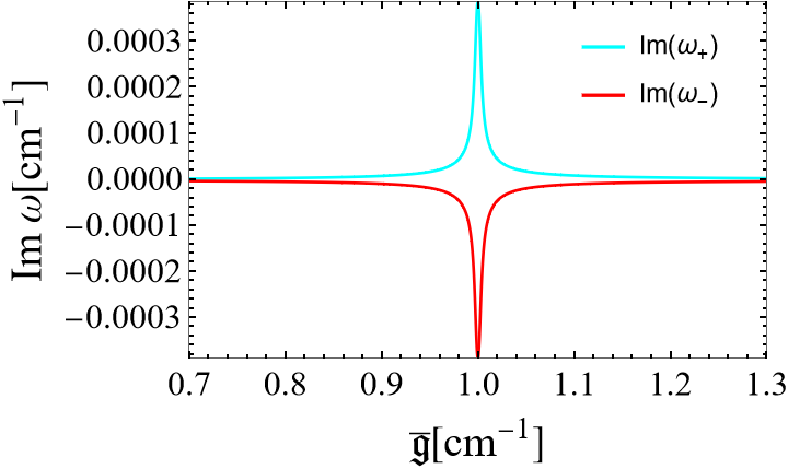
We plot the real and imaginary parts of $\omega$ for the two branches in Figs. 1 and 2, respectively, for the following parameter values: ${\color[rgb]{0,0,0}\mathfrak{g}}=1\,\mathrm{cm}^{-1},\ \gamma=2.05\times 10^{-7}\,\mathrm{cm}^{-1},\ \alpha=-4.5\times 10^{-8}\,\mathrm{cm}^{-1}$. In these plots we take $\bar{{\color[rgb]{0,0,0}\mathfrak{g}}}$ as a free parameter. It is apparent from the plots of imaginary part that there is a rather narrow region of $\bar{g}$, in which the growth rate is enhanced roughly by two orders of magnitude. This is the resonance-like structure that Ref. Xiong et al. 2022 first pointed out and we will focus on in this paper. In fact, the resonance-like peak occurs near the point, at which the real parts of $\omega_{+}$ and $\omega_{-}$ come close to each other. Note that although the resonance-like structure was reported only for the isotropy-preserving modes in Ref. Xiong et al. 2022, it occurs also for the isotropy-breaking modes as shown in Fig. 2.

To locate where the enhancement occurs exactly, we differentiate $\omega_{+}({\color[rgb]{0,0,0}\mathfrak{g}},\ \bar{{\color[rgb]{0,0,0}\mathfrak{g}}},\ \Gamma,\ \bar{\Gamma})$ of the isotropy-preserving branch in Eq. 19 with respect to $\bar{{\color[rgb]{0,0,0}\mathfrak{g}}}$ as

where we define $C$ as

The imaginary part of the derivative vanishes at the unique value of $\bar{{\color[rgb]{0,0,0}\mathfrak{g}}}$ that corresponds to $A^{2}=\alpha^{2}$. Thus the resonance-like peak occurs when $|A|\approx|\alpha|$, i.e., the number densities of neutrino and antineutrino come close to each other. Note that the difference between $\Gamma$ and $\bar{\Gamma}$ is usually orders of magnitude smaller than the difference between $g$ and $\bar{g}$, i.e., $|\alpha|\ll|A|$.

In the isotropy-preserving branch, the imaginary part of $\omega_{+}$ is given approximately as

In the situation of our concern, where ${\color[rgb]{0,0,0}\mathfrak{g}},\bar{{\color[rgb]{0,0,0}\mathfrak{g}}}\gg\Gamma,\bar{\Gamma}$, the first case is non-resonant, since $G\gg|\alpha|$. On the other hand, the second case may fall in the resonance-like region. Note that the imaginary part is positive in the second regime unless $\alpha$ is much smaller than $\gamma$. In the first regime, on the other hand, the signature of the imaginary part is determined by the competition of difference between $g$ and $\bar{g}$ and that between $\Gamma$ and $\bar{\Gamma}$.

Although we have so far regarded $\omega$ as a function of $\bar{{\color[rgb]{0,0,0}\mathfrak{g}}}$, one can also take other parameters. If one varies ${\color[rgb]{0,0,0}\mathfrak{g}}$ instead of $\bar{{\color[rgb]{0,0,0}\mathfrak{g}}}$, the same criterion $|A|\approx|\alpha|$ is obtained. This resonance-like peak, if regarded as a function of one of the collision rates, it reaches the maximum height at a certain value of this rate. Note also that the resonance-like peak occurs at ${\color[rgb]{0,0,0}\mathfrak{g}}\sim\bar{{\color[rgb]{0,0,0}\mathfrak{g}}}$ but not exactly at ${\color[rgb]{0,0,0}\mathfrak{g}}=\bar{{\color[rgb]{0,0,0}\mathfrak{g}}}$. To see this more clearly, we choose a different parameter set, in which we artificially raise the collision rate of antineutrinos to an unrealistically high value $\bar{\Gamma}=0.025\ \mathrm{cm}^{-1}$ so that $|\alpha|\approx 0.025\ \mathrm{cm}^{-1}$. We then obtain $\bar{{\color[rgb]{0,0,0}\mathfrak{g}}}\approx 1.025\ \mathrm{cm}^{-1}$ at the peak. This deviation from ${\color[rgb]{0,0,0}\mathfrak{g}}=1\ \mathrm{cm}^{-1}$ is confirmed in Fig. 1. One should also notice that the peak amplitude in the resonance-like structure is much larger, and the peak width is also much broader in this extreme case. A similar analysis shows that the resonance-like structure occurs also for the isotropy-breaking branch. The peak location is a bit different from that for the isotropy-preserving mode and satisfies $A^{2}=(3\alpha)^{2}$, as demonstrated in Fig. 2 again for the exaggerated value of $\bar{\Gamma}=0.025\ \mathrm{cm}^{-1}$. It is also observed that the peak width in the resonance-like structure for the isotropy-breaking mode is not appreciably different from that for the isotropy-preserving mode whereas the peak amplitude is smaller by a factor $\sim 2$ for the isotropy-breaking mode than that for the isotropy-preserving mode.

So far we have employed the dispersion relation. The behavior discussed above can be also derived directly from the original quantum kinetic equation. Since it provides a different insight into the resonance-like structure, we will look at it below. We assume that the background is homogeneous, isotropic, and monochromatic. The vacuum and matter terms are ignored to focus on CFI. Then the Hamiltonian and the collision term are given as

Note that the Hamiltonian is divided into the diagonal part $H_{\text{d}}$ and the off-diagonal part $H_{\text{o}}$. The equilibrium distributions are set to the unperturbed states:

The linearized equations for $S$ and $\bar{S}$ are given as

where $\bm{V}$ is vector defined as

and $\bm{W}$ is the matrix expressed as

Note that we assume that the perturbation is also isotropic in deriving these equations here.

The general solution is given as the superposition of two independent solutions:

where $\bm{V}_{\pm},\ \omega_{\pm}$ are the eigenvectors and eigenvalues to the matrix $W$. The eigenvalues are obtained as Lin and Duan 2022

where the notations are identical to those for Eq. 19.

It is interesting to point out that the elimination of the diagonal part of the Hamiltonian does not change the two eigenvalues, which suggests that CFI is driven by an interplay of the off-diagonal part of the Hamiltonian and the collision terms. That may be illuminated more clearly by treating the collision term as a perturbation. Les us first consider the case with $H=H_{\text{o}}$ and no collision term, $C=0$. The eigenvalues and eigenvectors in this case are given as

where and below we introduce the following notations:

This is a stable flavor evolution with no growth of amplitudes.

Now we reinstate the collision terms but as a perturbation. The characteristic equation is then written as

where the eigenvalue is expressed as the sum of the unperturbed value given in Eq. 35 and a (small) shift. To the linear order, the shifts are obtained for the two modes as

They are divergent at ${\color[rgb]{0,0,0}\mathfrak{g}}=\bar{{\color[rgb]{0,0,0}\mathfrak{g}}}$ unless $\Gamma=\bar{\Gamma}$, an indication of the resonance-like structure in the current setting, i.e., the collision term is assumed to be small and so is the shift, the latter of which is no longer correct at $g\approx\bar{g}$, however. Note that the two shifts have opposite signatures, in qualitative agreement with the exact solution.

Now we go beyond the linear analysis. We solve the quantum kinetic equation

for the homogeneous, isotropic, and monochromatic neutrino distributions. The vacuum and matter terms are omitted again. The following simulations are meant to study the nonlinear evolution of the isotropy-preserving mode both outside and in the resonance-like regions. For this purpose we vary rather arbitrarily $\bar{{\color[rgb]{0,0,0}\mathfrak{g}}}$, the distribution function of antineutrino. For comparison, we also run linear simulations, in which the Hamiltonian is fixed to the initial value.

Since the vacuum term, which would produce perturbations to the flavor eigenstate automatically, is neglected here, we give an initial perturbation by hand as follows:

For simplicity, we assume that all neutrinos are initially in the electron flavor and the initial perturbation is isotropic so that the isotropy-breaking mode does not appear in this simulation. As discussed in the previous section, the occurence of CFI is dictated by the four quantities: ${\color[rgb]{0,0,0}\mathfrak{g}},\ \bar{{\color[rgb]{0,0,0}\mathfrak{g}}},\ \Gamma$ and $\bar{\Gamma}$ (see Eq. 36). Note that in the linear simulations, ${\color[rgb]{0,0,0}\mathfrak{g}}$ and $\bar{{\color[rgb]{0,0,0}\mathfrak{g}}}$ are conserved quantities and unchanged in time.

The collision rates are chosen as

which correspond to

Since the $\Gamma$ and $\bar{\Gamma}$ are much smaller than ${\color[rgb]{0,0,0}\mathfrak{g}}$ and $\bar{{\color[rgb]{0,0,0}\mathfrak{g}}}$, the resonance-like peak occurs essentially at ${\color[rgb]{0,0,0}\mathfrak{g}}=\bar{{\color[rgb]{0,0,0}\mathfrak{g}}}$.

The results of the linear simulations are shown first in Fig. 3 for three different values of $\bar{{\color[rgb]{0,0,0}\mathfrak{g}}}$: $1.000\,\mathrm{cm}^{-1},1.009\,\mathrm{cm}^{-1}$ and $1.100\ \mathrm{cm}^{-1}$. The first one almost corresponds to the resonance-like peak whereas the second and third values give the edge of and a point outside the resonance-like region, respectively. The blue curves are the modulus of flavor coherence, $|S|$, plotted against time while the yellow lines indicate for comparison the exponential growths with the values of $\omega_{+}$ given in Eq. 19 for these settings. As should be clear, $|S|$ shows the exponential growth as expected in all cases. In particular, the growth is much faster indeed in the resonance-like region. Note also that the initial conditions are not exactly the eigenmodes corresponding to $\omega_{+}$ and some deviations from the exact exponential growth are seen.

Now we procced to the results of the fully nonlinear simulations run for the first two initial conditions employed in the linear simulations presented just above. They correspond to the peak and edge of the resonance-like structure, respectively. In Fig. 4 we plot not only $|S|$, the modulus of the flavor coherence and the off-diagonal component of the density matrix, but also the distribution functions of all neutrinos, which are also the diagonal components of the density matrix, as functions of time. For reference, the exponential growths with the values of $\omega_{+}$ in Eq. 19 for the current settings are again exhibited.

One recognizes clearly that there are two distinct phases, the linear phase, in which the flavor coherence grows exponentially at the rate given in the linear analysis, and the nonlinear saturation phase, where the $|S|$ peaks out and levels off thereafter and the distribution functions of neutrinos and antineutrinos are also settled gradually to states that are steady in the statistical sense and are different from the initial ones (see the insets in each panel). The transition from the linear phase to the nonlinear phase may be characterized by $|S|\sim\mathfrak{g}$. It is found from the result in the resonance-like structure that the saturation level of the flavor coherence is not particularly large (actually smaller) compared with the case for the edge of the resonance-like region and that the role of resonance-like phenomenon is just to shorten the time it takes to reach the saturation.

This may be supported by another simulation, a variant of the second case, in which the $\bar{\Gamma}$ is changed to $3.6\times 10^{-7}\ \mathrm{cm}^{-1}$ with other parameters, particularly ${\color[rgb]{0,0,0}\mathfrak{g}}$ and $\bar{{\color[rgb]{0,0,0}\mathfrak{g}}}$, fixed so that it should give the point closer to the resonance-like peak. The result is presented as Fig. 4. Note that the linear growth rate is twice as large as that in the second case and is close to that in the first case. The saturation occurs earlier consistently with the enhanced linear growth rate. On the other hand, the asymptotic state is almost the same as that in the second case. It is mostly determined by the initial neutrino distributions and little affected by the resonance-like phenomenon.

It shold be noted that the asymptotic state may be oscillating in time and is steady not in the literal sense but in the statistical sense. The substantially smaller populations of $\nu_{x}$ and $\bar{\nu}_{x}$ in the asymptotic states in these models are the consequence of our choice of the equilibrium state in the relaxation approximation adopted in the simulation and are rather artificial. It should be also mentioned that in reality, where the background matter and neutrinos themselves may change significantly due to advection over the time scale of neutrino oscillations, the asymptotic state may never be reached. It was found that CFI could win the compitition against advection (see Xiong et al. 2023). What consequences the accelerated saturation may have, if any, for the core-collapse supernova remain to be studied.

It is interesting to point out that in the first case corresponding approximately to the resonance-like peak, a very fast flavor bouncing occurs in the beginning of the nonlinear saturation phase right after the peak-out. It is due to the diagonal part of the collision term, in which the equilibrium distributions is imposed. In fact, if we reset the equilibrium values to the actual asymptotic values when the nonlinear phase is reached, this feature disappears.

We assume that neutrinos and antineutrinos have continuous energy spectra given by the Fermi-Dirac distributions:

where $g_{i}$, $T_{i}$ and $\mu_{i}$ are the model parameters for the neutrino species $i$, and $E$ is the neutrino energy. Assuming for simplicity that only electron flavor is present initially, we choose

and the shorthand notation

will be used in the following; the temperatures are set to

we further assume that $\mu=0$. Although it is not presented here, we confirmed that a non-zero $\mu$ does not change qualitatively the result in the following. The collision term is now assumed to depend on the energy quadratically as

with

common to all flavors.

For later convenience we introduce the number density multiplied by $\sqrt{2}G_{\mathrm{F}}$, $n_{i}$, the mean energy, $\langle E\rangle_{i}$, and the mean collision rate, $\langle\Gamma\rangle_{i}$ for the neutrino species $i$ as

These three quantites defined above have same unit. Note that a change in $g_{i}$ influences only $n_{i}$ while a variation in $T_{i}$ or $\mu_{i}$ influences all of $n_{i},\ \langle E\rangle_{i},\ \langle\Gamma\rangle_{i}$. We also introduce the following quantities:

We solve Eq. 15 numerically to obtain the dispersion relation. In doing so, the energy range from $0\ \mathrm{MeV}$ to $80\ \mathrm{MeV}$ is divided into nonuniform 128 bins concentrated more at low energies.

We plot in Fig. 5 the contour lines for $\mathrm{Re}\ I=-1$ or $3$ (blue) and $\mathrm{Im}\ I=0$ (orange) in the complex $\omega$ plane for some representative values of $\bar{g}$. The intersection of the two contour lines gives the dispersion relation $\omega(k)$ at $k=0$. One of the two solutions (except for the origin) with a positive imaginary part is the unstable mode. The first three plots in the figure are for the isotropy-preserving branch at $\bar{g}=0.51,\ 0.511,\ 0.512$, respectively, and the last plot is for the isotropy-breaking branch at $\bar{g}=0.512$. For the current choice of parameters, which correspond to

the resonance-like peak is expected to occur approximately at $\bar{g}=0.512$ (panels (c) and (d)) giving $n\approx\bar{n}\approx 4.88691\ \mathrm{cm}^{-1}$.

This is confirmed in Fig. 6, where we plot the real and imaginary parts of $\omega$ for the unstable isotropy-preserving branch as a function of $\bar{g}$. One can see a familiar enhancement of the imaginary part, or the growth rate of the instability.

We also investigate an extreme case, in which we artificially magnify the collision rate $\bar{\Gamma}$ of antineutrino by five orders of magnitude, $\Gamma_{0}=1\ \mathrm{cm}^{-1}$ in Eq. 48, while other parameters are unchanged. This gives $\alpha=-1.6174\ \mathrm{cm}^{-1}$. The result is shown in Fig. 6. The resonance-like peak occurs at $\bar{g}=0.74$, which corresponds to $A=-1.0081\ \mathrm{cm}^{-1}$. The number density of antineutrino is noticably different from that of neutrino in this case just as inferred from the result of the monochromatic case. Again the approximate formula (orange line) is compared with the numerical result shown in blue. This time the approximation is not so successful as before although the peak shift as well as the broadening of resonance-like region are captured qualitatively. It is pointed out that thanks to this broadening the case with $n=\bar{n}$ is still in the resonance-like region, although not at the peak, and hence the growth rate is enhanced. We explored other neutrino spectra, such as the Fermi-Dirac distributions with non-vanishing chemical potentials or the Gaussian and polynomial distributions that are not too irregular. The results are qualitatively the same as those given above and hence will not be presented here.

Finally, it is worth pointing out that the growth rate of the resonance-like structure is well approximated by the formula for the monochromatic case, Eq. 19 for $\omega_{+}$, with the following substitutions:

Note that this approximate formula agrees with the one derived previously in Xiong et al. 2022 under the assumption of $|\Gamma|,\ |\bar{\Gamma}|\ll|\omega|$ if $\gamma$ and $\alpha^{2}$ are neglected accordingly. This is demonstrated in Fig. 6, where the numerical solution displayed in blue is compared with the approximate one presented in orange. Their agreement matches what was shown in Xiong et al. 2022. Although the criterion for resonance-like phenomenon posited in that paper is appropriate only when the collision rates are small, the condition $|A|\sim|\alpha|$ is always satisfied at the resonance-like peak regardless of the parameter values.

We again solve Eq. 39 numerically for homogeneous and isotropic neutrinos with the Fermi-Dirac distributions as the energy spectra. The background distributions are actually the same as those employed for the linear analysis in the previous section, Eqs. 44-48. Since the vacuum term is omitted in the kinetic equation, we need to set an initial perturbation by hand, which is also assumed to be isotropic and homogeneous. Hence only the isotropy-preserving branch is considered. We take $\bar{g}$ as a free parameter and vary it so that the unperturbed state should be either near the resonance-like peak or near the edge of the resonance-like region.

In the simulation, the energy range from $1\ \mathrm{MeV}$ to $100\ \mathrm{MeV}$ is divided uniformly into 100 bins this time. We adopt the following initial perturbations only to the off-diagonal components of the density matrix

The numbers in the functions are chosen rather arbitrarily.

The results of the linear simulations, in which the Hamiltonian is fixed to the initial value, is shown in Fig. 7 for two choices of $\bar{g}$, one corresponding approximately to the resonance-like peak and the other giving the edge of the resonance-like region. The value of $A/\alpha$ measures how close the initial configuration is to the resonance-like peak: the closer to unity it is, the nearer to the resonance-like peak the initial state is. It is evident that the flavor coherence grows at a common rate for all energies Lin and Duan 2022, just as expected from the energy-independent nature of $\omega(k)$. In the resonance-like region, it grows much faster indeed.

The corresponding results for the nonlinear simulations are presented in Figs. 8 and 9. Again one recognizes that the linear phase is followed by the nonlinear saturation phase also in this case with the non-monochromatic energy spectra. In the linear phase the flavor coherence grows at a common rate for all energies just as in the linear simulations given above (see Fig. 8). In the case for the resonance-like peak (panel (a)), the nonlinear phase is reached much faster than in the case for the edge of the resonance-like region (panel (b)).

It is also found that the beginning of the nonlinear phase is marked for each energy when $|S(E)|=f(E)$ is satisfied individually, which is a direct extension of the monochromatic case. The saturation level is not much different between the two cases (see Fig. 9), indicating again that the main effect of the resonance-like phenomenon is to accelerate the linear growth and the asymptotic state is hardly affected. The bouncing in the nonlinear phase is observed only for the resonance-like peak. The bouncing amplitude seems to be related with the difference between the equilibrium distribution and the asymptotic distribution although the exact mechanism of bouncing is not clear at the moment. This is induced by the diagonal part of the collision term. In fact, if we discard the diagonal part effectively by resetting the equilibrium distributions to the asymptotic ones, the bouncing feature is gone just as in the monochromatic case.

In this last section, we investigate the resonance-like structure either for $k\neq 0$ perturbations in the homogeneous and isotropic background or for $k=0$ modes in the homogeneous but anisotropic background. We work on the dispersion relations in the linear regime. The neutrino energy spectra are again assumed to be the Fermi-Dirac distributions given in Eq. 43, with the same parameters as in Eqs. 44-46 and, in addition, with $\bar{g}=g_{\bar{\nu}_{e}}=0.512$, corresponding to the resonance-like peak at $k=0$. The collision rates are given by Eqs. 47-48.

We begin with the $k\neq 0$ perturbation in the homogeneous and isotropic background. In the following the wave vector $\bm{k}$ is assumed to be parallel to the z-axis. We solve Eq. 14 numerically to obtain the dispersion relation. For $k\neq 0$, there appear two nonvanishing off-diagonal components in $\Pi_{ex}$ in addition to the diagonal ones, which survive in the $k\rightarrow 0$ limit. In order to see how the isotropy-preserving and isotropy-breaking branches at $k=0$ are mixed with each other to new modes in the $k\neq 0$ case, we decompose $\Pi_{ex}$ as

Then its determinant can be written explicitly in a simple form as

where the following relations

are used. Note that in the limit of $k=0$, the following relations hold further:

and the dispersion relation is obtained from

In fact, the isotropy-preserving branch is derived from the first factor and the isotropy-breaking branch is originated from the second factor. In the case of $k\neq 0$, while $A^{11}-1=0$ is unchanged, $(A^{00}+1)(A^{11}-1)-(A^{03})^{2}=0$ now mixes the isotropy-preserving and isotropy-breaking branches to produce four branches in general. In the following we look into these modes in detail.

From the first factor in Eq. 55, a pair of solutions are obtained, which take the following form $a=(0,a_{x},a_{y},0)$ and is perpendicular to $\bm{k}$, and they hence break the isotropy in the $x-y$ plane. On the other hand, the second factor can vanish in three different manners: $(1)A^{00}+1=A^{03}=0,\ (2)A^{33}-1=A^{03}=0$, or $(3)(A^{00}+1)(A^{33}-1)=(A^{03})^{2}\neq 0$. The first case produces a solution of the form: $a=(a_{t},0,0,0)$, which is isotropy-preserving. The second case leads to $a=(0,0,0,a_{z})$, which is hence isotropy-breaking in the z direction, that is, the direction of $\bm{k}$. The last one yields a solution with the form of $a=(a_{t},0,0,a_{z})$ in general, which is also isotropy-breaking. If the first and second factors vanish simultaneously, the solution takes a combined form: for example, the combination of the first factor with case (1) for the second factor gives a solution of the following form: $a=(a_{t},a_{x},a_{y},0)$. These cases are exceptional, though, and occur only for special spectra/collision rates. In fact, we find that case (3) is always satisfied in the second factor of Eq. 55 for the ranges of $k$ and $\bar{g}$ considered in this paper.

In Fig. 10, we display plots of the contours indicated in each panel for $k=0.001\,\mathrm{cm}^{-1}$. The left panel gives the solutions for the first factor in Eq. 55 whereas the right panel shows the solutions for the second factor. The latter corresponds to case (3) as mentioned above. At this small $k$, all the modes are not much different from the counterparts at $k=0$. For later convenience, we refer to the solutions for unstable modes in these plots as Q, W, and Y. Mode Q originated from the first factor in Eq. 55 merges at $k=0$ with Y from the second factor to give the isotropy-breaking modes. On the other hand, mode W is reduced to the isotropy-preserving mode at $k=0$. These modes are all isotropy-breaking at $k\neq 0$. In Fig. 11 we plot the linear growth rates, $\mathrm{Im}\,\omega$, for these three modes as a function of $\bar{g}$ at the same value of $k=0.001\,\mathrm{cm}^{-1}$. The resonance-like structure is evident in all cases around $\bar{g}=0.512$.

In Fig. 12, we show the $k$-dependence of these growth rates at $\bar{g}=0.512$, i.e., around the resonance-like peak. It is apparent that they decrease monotonically with $k$, indicating that the resonance-like peak gets weaker at non-vanishing $k$ for all modes. This is actually true outside the resonance-like region as well. The non-zero $k$ tends to reduce the CFI itself. It is noted that the presence of $\bm{k}$ in the denominator of Eq. 14 poses a challenge in the numerical integration by discretization in the region $-k<\mathrm{Re}\,\omega<k,\ 0<\mathrm{Im}\,\omega<\Gamma(E_{max})$. We do not think that the numerical solutions in these ranges are reliable and hence do not consider those solutions outside the resonance-like region or inside it but at large values of $k$ that approach this problematic region, which is indicated as the gray bands around the origin in Fig.10.

Next we study the effect of the anisotropy in the homogeneous neutrino background on the resonance-like structure. We introduce the following angular-dependence to the neutrino distributions in momentum space:

where $f_{i}(E,\,g_{i},\,T_{i},\,\mu_{i})$ on the right hand side is the Fermi-Dirac distribution for neutrino species $i$; $0<\theta<\pi$ is the angle that the neutrino velocity makes with the radially outward direction; the factor $\delta_{i}$ controls the degree of anisotropy. Since we are interested in the resonance-like structure in CFI in this paper, we first consider a case with no angular crossing, and hence no FFC. We then look at two cases with different angular crossings to see the interplay between the resonance-like structure in CFI and FFC. We solve Eq. 14 numerically for $k=0$ to obtain the dispersion relation $\omega(k=0)$ for the anisotropic (but homogeneous) background just described. Note that the integration over the solid angle can be done analytically for $k=0$.

We first present the results for the first case, in which only electron-type neutrinos and antineutrinos are present initially with the same anisotropy: $\delta=\bar{\delta}$. We choose the model parameters as in Eqs. 44-48 together with $\bar{g}=0.512$ and $k=0$ so that the unperturbed state corresponds to the resonance-like peak at $\delta=0$. We vary the value of $\delta$ to see how the anisotropy affects CFI in the resonance-like region. The choice of $k=0$ simplifies the analysis a lot. In fact, only $\Pi_{ex}^{03}$, which is linear in $\delta$, is non-vanishing as the off-diagonal components of $\Pi_{ex}$ just as in the previous case with $k\neq 0$, and the diagonal components are unchanged from those for the isotropic case. Since the dispersion relation is obtained from $\mathrm{det}\,\Pi_{ex}{\color[rgb]{0,0,0}=0}$ given as Eq. 55 again, we refer to the corresponding modes as Q, W, and Y. Under the current setting, all modes are isotropy-breaking for $\delta\neq 0$. Note that mode Q is independent of $\delta$ and $\bar{\delta}$ in this setting, and is always identical to the isotropy-breaking mode for isotropic neutrinos.

References

- Pantaleone (1992) J. Pantaleone, Dirac neutrinos in dense matter, Phys. Rev. D 46, 510 (1992).
- Sigl and Raffelt (1993) G. Sigl and G. Raffelt, General kinetic description of relativistic mixed neutrinos, Nuclear Physics 406, 423 (1993).
- Duan et al. (2010) H. Duan, G. M. Fuller, and Y.-Z. Qian, Collective neutrino oscillations, Annual Review of Nuclear and Particle Science 60, 569 (2010), https://doi.org/10.1146/annurev.nucl.012809.104524 .
- Chakraborty et al. (2016) S. Chakraborty, R. Hansen, I. Izaguirre, and G. Raffelt, Collective neutrino flavor conversion: Recent developments, Nuclear Physics B 908, 366 (2016), neutrino Oscillations: Celebrating the Nobel Prize in Physics 2015.
- Tamborra and Shalgar (2021) I. Tamborra and S. Shalgar, New developments in flavor evolution of a dense neutrino gas, Annual Review of Nuclear and Particle Science 71, 165 (2021), https://doi.org/10.1146/annurev-nucl-102920-050505 .
- Richers and Sen (2022) S. Richers and M. Sen, Fast flavor transformations (2022).
- Morinaga (2022) T. Morinaga, Fast neutrino flavor instability and neutrino flavor lepton number crossings, Phys. Rev. D 105, L101301 (2022).
- Abbar et al. (2019) S. Abbar, H. Duan, K. Sumiyoshi, T. Takiwaki, and M. C. Volpe, On the occurrence of fast neutrino flavor conversions in multidimensional supernova models, Phys. Rev. D 100, 043004 (2019).
- Nagakura et al. (2019) H. Nagakura, T. Morinaga, C. Kato, and S. Yamada, Fast-pairwise collective neutrino oscillations associated with asymmetric neutrino emissions in core-collapse supernovae, The Astrophysical Journal 886, 139 (2019).
- Delfan Azari et al. (2020) M. Delfan Azari, S. Yamada, T. Morinaga, H. Nagakura, S. Furusawa, A. Harada, H. Okawa, W. Iwakami, and K. Sumiyoshi, Fast collective neutrino oscillations inside the neutrino sphere in core-collapse supernovae, Phys. Rev. D 101, 023018 (2020).
- Abbar et al. (2020) S. Abbar, H. Duan, K. Sumiyoshi, T. Takiwaki, and M. C. Volpe, Fast neutrino flavor conversion modes in multidimensional core-collapse supernova models: The role of the asymmetric neutrino distributions, Phys. Rev. D 101, 043016 (2020).
- Morinaga et al. (2020) T. Morinaga, H. Nagakura, C. Kato, and S. Yamada, Fast neutrino-flavor conversion in the preshock region of core-collapse supernovae, Phys. Rev. Res. 2, 012046 (2020).
- Glas et al. (2020) R. Glas, H.-T. Janka, F. Capozzi, M. Sen, B. Dasgupta, A. Mirizzi, and G. Sigl, Fast neutrino flavor instability in the neutron-star convection layer of three-dimensional supernova models, Phys. Rev. D 101, 063001 (2020).
- Abbar (2020) S. Abbar, Searching for fast neutrino flavor conversion modes in core-collapse supernova simulations, Journal of Cosmology and Astroparticle Physics 2020 (05), 027.
- Capozzi et al. (2021) F. Capozzi, S. Abbar, R. Bollig, and H.-T. Janka, Fast neutrino flavor conversions in one-dimensional core-collapse supernova models with and without muon creation, Phys. Rev. D 103, 063013 (2021).
- Nagakura et al. (2021) H. Nagakura, A. Burrows, L. Johns, and G. M. Fuller, Where, when, and why: Occurrence of fast-pairwise collective neutrino oscillation in three-dimensional core-collapse supernova models, Phys. Rev. D 104, 083025 (2021).
- Harada and Nagakura (2022) A. Harada and H. Nagakura, Prospects of fast flavor neutrino conversion in rotating core-collapse supernovae, The Astrophysical Journal 924, 109 (2022).
- Akaho et al. (2022) R. Akaho, A. Harada, H. Nagakura, W. Iwakami, H. Okawa, S. Furusawa, H. Matsufuru, K. Sumiyoshi, and S. Yamada, Protoneutron star convection simulated with a new general relativistic boltzmann neutrino radiation-hydrodynamics code (2022).
- Martin et al. (2021) J. D. Martin, J. Carlson, V. Cirigliano, and H. Duan, Fast flavor oscillations in dense neutrino media with collisions, Phys. Rev. D 103, 063001 (2021).
- Sigl (2022) G. Sigl, Simulations of fast neutrino flavor conversions with interactions in inhomogeneous media, Phys. Rev. D 105, 043005 (2022).
- Johns and Nagakura (2022) L. Johns and H. Nagakura, Self-consistency in models of neutrino scattering and fast flavor conversion, Phys. Rev. D 106, 043031 (2022).
- Shalgar and Tamborra (2021) S. Shalgar and I. Tamborra, Change of direction in pairwise neutrino conversion physics: The effect of collisions, Phys. Rev. D 103, 063002 (2021).
- Kato et al. (2021) C. Kato, H. Nagakura, and T. Morinaga, Neutrino transport with the monte carlo method. ii. quantum kinetic equations, The Astrophysical Journal Supplement Series 257, 55 (2021).
- Sasaki and Takiwaki (2022) H. Sasaki and T. Takiwaki, A detailed analysis of the dynamics of fast neutrino flavor conversions with scattering effects, Progress of Theoretical and Experimental Physics 2022, 10.1093/ptep/ptac082 (2022), 073E01, https://academic.oup.com/ptep/article-pdf/2022/7/073E01/44400755/ptac082.pdf .
- Hansen et al. (2022) R. S. L. Hansen, S. Shalgar, and I. Tamborra, Enhancement or damping of fast neutrino flavor conversions due to collisions, Phys. Rev. D 105, 123003 (2022).
- Kato and Nagakura (2022) C. Kato and H. Nagakura, Effects of energy-dependent scatterings on fast neutrino flavor conversions, Physical Review D 106, 10.1103/physrevd.106.123013 (2022).
- Padilla-Gay et al. (2022) I. Padilla-Gay, I. Tamborra, and G. G. Raffelt, Neutrino fast flavor pendulum. ii. collisional damping, Phys. Rev. D 106, 103031 (2022).
- Capozzi et al. (2019) F. Capozzi, B. Dasgupta, A. Mirizzi, M. Sen, and G. Sigl, Collisional triggering of fast flavor conversions of supernova neutrinos, Phys. Rev. Lett. 122, 091101 (2019).
- Johns (2021) L. Johns, Collisional flavor instabilities of supernova neutrinos (2021).
- Johns and Xiong (2022) L. Johns and Z. Xiong, Collisional instabilities of neutrinos and their interplay with fast flavor conversion in compact objects, Phys. Rev. D 106, 103029 (2022).
- Lin and Duan (2022) Y.-C. Lin and H. Duan, Collision-induced flavor instability in dense neutrino gases with energy-dependent scattering (2022).
- Xiong et al. (2023) Z. Xiong, M.-R. Wu, G. Martínez-Pinedo, T. Fischer, M. George, C.-Y. Lin, and L. Johns, Evolution of collisional neutrino flavor instabilities in spherically symmetric supernova models, Phys. Rev. D 107, 083016 (2023).
- Xiong et al. (2022) Z. Xiong, L. Johns, M.-R. Wu, and H. Duan, Collisional flavor instability in dense neutrino gases (2022).
- Airen et al. (2018) S. Airen, F. Capozzi, S. Chakraborty, B. Dasgupta, G. Raffelt, and T. Stirner, Normal-mode analysis for collective neutrino oscillations, Journal of Cosmology and Astroparticle Physics 2018 (12), 019.
- Izaguirre et al. (2017) I. Izaguirre, G. Raffelt, and I. Tamborra, Fast pairwise conversion of supernova neutrinos: A dispersion relation approach, Phys. Rev. Lett. 118, 021101 (2017).
- Zaizen and Nagakura (2022) M. Zaizen and H. Nagakura, Simple method for determining asymptotic states of fast neutrino-flavor conversion, arXiv e-prints , arXiv:2211.09343 (2022), arXiv:2211.09343 [astro-ph.HE] .
- Shalgar and Tamborra (2019) S. Shalgar and I. Tamborra, On the occurrence of crossings between the angular distributions of electron neutrinos and antineutrinos in the supernova core, The Astrophysical Journal 883, 80 (2019).
- Shalgar and Tamborra (2022) S. Shalgar and I. Tamborra, Neutrino flavor conversion, advection, and collisions: The full solution (2022).