Topology of the landscape and dominant kinetic path for the thermodynamic phase transition of the charged Gauss-Bonnet AdS black holes
Abstract
We study the generalized free energy of the five dimensional charged Gauss-Bonnet AdS black holes in the grand canonical ensemble by treating the black hole radius and the charge as the order parameters. On the two dimensional free energy landscape, the lowest points in the basins represent the local stable black holes and the saddle point represents the unstable black hole. We show that black hole is the topological defect of gradient field of the landscape. The black hole stability is determined by the topography of the free energy landscape in terms of the basin depths and the barrier height between the basins and is not by the topology of the gradient field. In addition, we study the stochastic dynamics of the black hole phase transition and obtain the dominant kinetic path for the transition on the free energy landscape. Unlike the one dimensional landscape, the dominant kinetic path between the small and the large black hole state does not necessarily pass through the intermediate black hole state. Furthermore, the inhomogeneity in diffusions can lead to the switching from the coupled cooperative process of black hole phase transition to the decoupled sequential process, giving different kinetic mechanisms.
I Introduction
Recently, the concept of the generalized free energy has been proposed to investigate the thermodynamics and the kinetics of the black hole phase transition Li:2020khm; Li:2020nsy. In this aspect, the key ingredient is to introduce the order parameter of the phase transition that describes the microscopic degrees of freedom at the coarse-grained level Wei:2015iwa; Wei:2019uqg. It is also shown that the generalized free energy can be derived from the Euclidean gravitational action of the non-equilibrium black holes with the Euclidean conical singularities Li:2022oup. This derivation established a concrete foundation of the free energy landscape description of the thermodynamics of the black hole phase transition.
The free energy landscape can be explored to quantify the underlying topography such as the basin depths and the barrier height between the basins of the attraction GPT; FSW; JW; JWRMP. From the free energy landscape topography, one can easily read off the stabilities of the on-shell black holes. The reason is that, if there are several on-shell states at a fixed ensemble temperature, the thermodynalically favored state is given by the state with the smallest free energy. Another advantage of free energy landscape quantification is that it allows us to study the kinetics of the phase transition process by treating the landscape as the thermodynamical potential that provides the deterministic driving force and treating the interaction between the black hole system and the bath as the thermal fluctuations that provide the stochastic force. Based on these assumptions, the Markovian dynamics and the non-Markovian dynamics of the black hole phase transition have been investigated Li:2021vdp; Li:2022ylz; Li:2022yti.
In the previous works Li:2020khm; Li:2020nsy, the order parameter of the black hole is chosen to be the radius of the event horizon and the generalized free energy is defined as the function of a single variable or the order parameter. Then, the free energy landscape is represented as a one dimensional curve Wei:2020rcd; Li:2020spm; Wei:2021bwy; Cai:2021sag; Lan:2021crt; Li:2021zep; Yang:2021nwd; Mo:2021jff; Kumara:2021hlt; Li:2021tpu; Liu:2021lmr; Xu:2021usl; Du:2021cxs; Dai:2022mko; Luo:2022gss; Xu:2022jyp. In general, for other complex systems, for example, proteins in biophysics, chemical reaction systems, et.al. the free energy is the function of multiple order parameters and the landscape is intrinsically high dimensional JW; JWRMP. One question naturally raised is whether there is high dimensional landscape to describe the black hole phase transition.
In the present work, we consider the thermodynamic phase transition of the five dimensional charged Gauss-Bonnet black holes Boulware:1985wk; Cai:2001dz; Wiltshire:1985us; Cvetic:2001bk. It was shown in Cai:2013qga; Zou:2014mha that the small/large black hole phase transition, which exhibits analogy with the Van de Waals liquid-gas system Kubiznak:2012wp; Kubiznak:2014zwa; Kubiznak:2016qmn, holds in five-dimensional spherically symmetric charged Gauss-Bonnet-AdS black holes when its potential is fixed within the range of . Based on this observation, we work in the grand canonical ensemble and define the generalized free energy as the function of the black hole radius and the black hole charge. The corresponding free energy landscape can then be represented as an intrinsic two dimensional surface. As far as we know, this example is the only case that the two order parameters can be introduced and the free energy landscape is two dimensional.
The black hole states are represented as the points on the landscape, and the on-shell black hole states are the extremum points of the landscape. From the topography of the landscape, one can easily read off the stabilities of the on-shell black holes. We find that the thermodynamically stable Gauss-Bonnet black holes correspond to the lowest points in the sink on the landscape, while the unstable Gauss-Bonnet black hole corresponds to the saddle point. It should be mentioned that, in Ref.Wei:2022dzw, by introducing a parameter and an ancillary vector field , the authors argued that the positive and negative winding numbers of the defects correspond to the local thermodynamical stable and unstable black holes. In the present work, we propose that, in order to reveal the relation between the topology of the landscape and the stabilities of the on-shell black holes, one should investigate the intrinsic topological properties of the gradient field of the free energy landscape, even for the one dimensional landscape. We find that the black hole can be treated as the topological defects of the gradient field of the landscape, but there is no indication that the topology is relevant to the stabilities of the on-shell black holes. We emphasize that the stabilities of the black holes is completely determined by the topography of the landscape.
We also study the phenomenological description of the black hole phase transition based on the stochastic dynamics. Considering the black hole as the thermal entity, there should thermal fluctuation and particle number fluctuation in the grand canonical ensemble. Without those fluctuations, the local stable black holes will remain in the basin of the free energy landscape and no phase transition occurs. In analogy to the Van der Waals fluid-gas phase transition Malakhov:1994, if these fluctuations are taken into account, the local stable black hole will undergo a stochastic motion on the landscape, which can be effectively described by the Langevin equation for the trajectories or the Fokker-Planck equation for the time evolution of the associated probability equivalently. For the two dimensional free energy landscape as discussed in the present work, one can determine the dominant kinetic path for the stochastic motion on the landscape by using the path integral formalism of the stochastic dynamics. For the one dimensional landscape, the kinetic path between the small black hole state and the large black hole state must pass through the intermediate black hole state Liu:2021lmr. By minimizing the abbreviated action functional Landau; Wangprl2006; Faccioli2006; WangJCP2010, we show that the dominant kinetic path passes through the intermediate black hole state when the fluctuation is very small while at the finite fluctuations it does not necessarily pass through the intermediate black hole state. Furthermore, we find that the inhomogeneity in diffusions can lead to the switching from the coupled cooperative process of black hole phase transition to the decoupled sequential process, giving rise to different kinetic mechanisms.
This paper is arranged as follows. In Section II, we defined the generalized free energy of the charged Gauss-Bonnet black holes and discuss the corresponding landscape in the grand canonical ensemble. In Section III, we discuss the stabilities of the on-shell black holes from the topography of the landscape. In Section IV, we address the question of how to study the intrinsic topological properties of the landscape. In Section V, we study the dominant kinetic path of the phase transition by using the path integral formalism. The conclusion is presented in the last section.
II Free energy landscape of Gauss-Bonnet AdS black holes
In this section, we introduce the charged Gauss-Bonnet black holes in five dimensions and summarize the primary thermodynamics properties. Then, we will give the definition of the generalized free energy in the grand canonical ensemble, which is the function of the black hole radius and the charge. The corresponding landscape is also presented.
For our purpose, we consider the spherically symmetric charged Gauss-Bonnet AdS black hole in dimensions that is described by the line element Boulware:1985wk; Cai:2001dz; Wiltshire:1985us; Cvetic:2001bk
| (1) |
where the metric function is given by
| (2) |
and the line element of the unit 3-sphere in hyperspherical coordinates is given by
| (3) |
For the hyperspherical coordinates , and run over the range to , and runs over to . The volume of the hypersphere is .
In the expression of the metric function , the parameter is the black hole mass, the parameter is the charge of the black hole, and the pressure is defined in terms of the cosmological constant Kastor:2009wy; Dolan:2011xt. It should be noted that, in order to have a well-defined vacuum in the theory, the effective Gauss-Bonnet coefficient should satisfy the constraint Cai:2013qga; Zou:2014mha
| (4) |
The thermodynamics of this black hole has been comprehensively discussed Cai:2013qga; Zou:2014mha . Let us summarize the primary conclusions. The mass, the Hawking temperature, the entropy, and the electric potential of the event horizon can be expressed in terms of the black hole radius as Cai:2013qga; Zou:2014mha
| (5) |
In these expressions, we can observe that these thermodynamic quantities can be considered as the function of the black hole radius and the charge . It has been shown that, when , there exists the small/large black hole phase transition in the grand canonical ensemble Cai:2013qga; Zou:2014mha. In the following, we will investigate the phase transition in the framework of the free energy landscape.
We now define the generalized free energy function for the charge Gauss-Bonnet black holes in the grand canonical ensemble as York:1986it; Whiting:1988qr; Braden:1990hw
| (6) | |||||
Note that in the definition of the generalized free energy, the two parameter and are considered as the ensemble parameter. This is to say that and are the temperature and the chemical potential of the thermal and the particle bath that the system contacts with. They are adjustable and determined by the external environment or the bath. Therefore, in the grand canonical ensemble, the free energy function is defined as the function of black hole radius and charge and the corresponding landscape is intrinsically two dimensional.
In Fig.1, the two dimensional free energy landscape for the charged Gauss-Bonnet AdS black hole is plotted. In this plot, we have chosen the ensemble temperature and the chemical potential to be the same as the critical temperature and the critical chemical potential of the small/large black hole phase transition. We show that the landscape has two separated basins and the basins are connected by a saddle point. At the critical point of phase transition, the two basins have the same depths. Otherwise, the two basins have different depths depending on the ensemble temperature and the chemical potential.

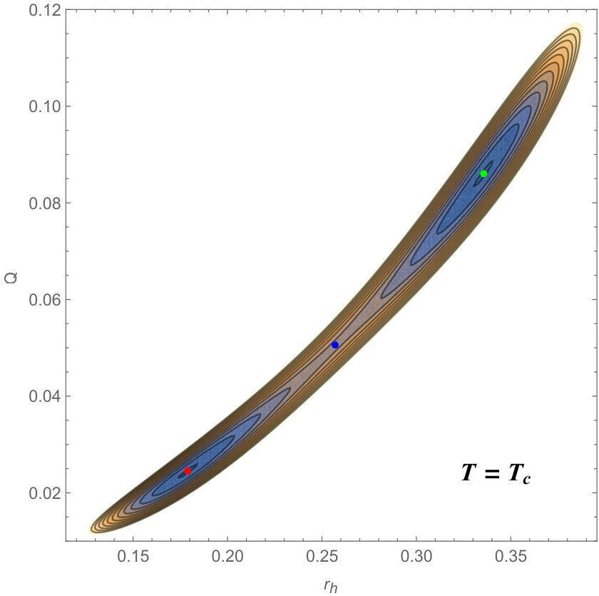
The corresponding two dimensional contour plot of the generalized free energy is presented in Fig.2. In this plot, there are three special points, i.e. the two lowest points in each basin and the saddle point, which are denoted by different colours. They are the extremum points on the landscape, which are determined by the necessary conditions for the extremum of the free energy function
| (7) |
It is easy to verify that the two conditions give rise to the expressions of the Hawking temperature and the electric potential in Eq.(II). This means that the three extremum points on the landscape represent the three branches of on-shell black hole solutions, and their Hawking temperature as well as the electrical potential are equal to those of the ensemble temperature and potential. The three branches of black holes are in equilibrium state with the bath. In this way, the necessary conditions (7) for the extremum are also the equilibrium conditions for the on-shell black holes.
III Stability of black hole from the topography of free energy landscape
In this section, we discuss the stabilities of the small/intermediate/large Gauss-Bonnet black holes from the topography of free energy landscape.
The generalized free energy provides us not only the free energies of the on-shell black holes, but also the free energies of the off-shell black holes. As mentioned, the equilibrium conditions Eq.(7), i.e. the extremum conditions for the landscape, lead to the expressions of the Hawking temperature and the electric potential of the on-shell black hole solutions. This is to say that the extremum points on the landscape just represent the on-shell black hole solutions, while other points represent the off-shell black hole states. From Fig.1 and Fig.2, we observe that the small, and the large black holes are represented by the lowest points of the basins on the landscape, and the intermediate black hole is represented by the saddle point.
In the plots of Fig.1 and Fig.2, the two basins have the same depths because the external parameters are selected to be the critical parameters of the black hole phase transition. Then, in this case, the small and the large black holes have the same on-shell free energies while the intermediate black hole has the higher free energy. Obviously, the small, and the large Gauss-Bonnet black holes are thermodynamically stable and the intermediate black hole is unstable.


One can also consider the case that the ensemble temperature is not equal to the critical temperature of phase transition. In Fig.3, the upper/bottom plot shows that the ensemble temperature is lower/higher than the critical temperature. In these two cases, the two basins on the landscape have different depths. The black hole state that is represented by the lowest point in the deeper basin is globally stable while the black hole state that is represented by the lowest point in the shallower basin is locally stable. From the plots, we can conclude that below the critical temperature the small black hole state is globally stable while above the critical temperature the larger black hole state is globally stable. The stabilities of the black holes are completely determined by the topography of the free energy landscape characterized by the basin depths and the barrier height between the basins. From the free energy landscape, one can easily read off the stabilities of the on-shell black holes.
IV The topology and defects of the free energy landscape
In this section, we discuss the recent proposal of treating black holes as topological defects. Recently, based on the concept of the generalized free energy, the topological properties of the thermodynamic parameter space was investigated in Ref.Wei:2022dzw. It is further argued that black hole can be treated as topological defect and the topological number can be used to characterize the stability of black hole. By introducing an ancillary parameter , the authors found some universal topological properties in the ”extended” parameter space. In particular, it is conjectured that the positive and negative winding numbers of the defects correspond to the local thermodynamical stable and unstable black holes. In this subsection, we will point out that there is an inconsistency in this proposal Liu:2022aqt; Fang:2022rsb.
More recently, another method was introduced to study the intrinsic topological properties of black hole thermodynamics Bai:2022klw. Using the spinodal curve, thermodynamic critical points of a black hole are endowed with the topological quantity of Brouwer degree. In addition, the topological transition between the different thermodynamic systems and the topological classification for them can be conveniently investigated. However, their analysis are not based on the free energy landscape. The relation between the topology of the free energy landscape and the stabilities of the on-shell black holes was not discussed.
Firstly, let us discuss whether the artificially introduced vector field in the space can be used to describe the topology of the landscape intrinsically Wei:2022dzw. Note that is an ancillary parameter. The intrinsic topology should not depend on the explicit form of the introduced vector field . It is obvious that, if we set the component of the vector field as an arbitrary positive definite function, the vector field has no zero point on the whole parameter space. Fig.4 shows the unit vector field for the Schwarzschild black holes when is set to be . There is no topological defects on the whole thermodynamic parameter space. Then, the winding number for arbitrary loop is zero. Therefore, the topological defect and the calculation of the winding number by using the ancillary parameter is not intrinsic. This conclusion is obviously valid for other types of black holes. The reason is that the generalized free energy in the canonical ensemble is intrinsically one dimensional and it only depends on the order parameter . The introduced parameter and the vector field have no significant physical meaning. It appears that the intrinsic topological properties of the parameter space cannot be revealed by the artificially introduced vector field .
Then, let us consider whether there is an intrinsic definition of topological defects based on the generalized free energy function. In canonical ensemble, the generalized free energy is the one variable function of the order parameter . One can naturally introduce the gradient field to describe the intrinsic topology of the free energy function. As an illustration, we consider the case of RNAdS black holes. In Fig.5, the free energy landscape and the gradient field of the RNAdS black hole are plotted. We can define an unit vector field as . Notice that this unit vector has singularities (where ) on the landscape. Obviously, these singularities can be treated as the topological defects according to Duan’s -mapping theory Duan. In addition, these singularities are just the on-shell black hole solutions. Therefore, black hole solutions can be treated as the topological defects of the gradient field of the free energy function, because the on-shell black hole solutions correspond to the zero points of the gradient field on the free energy landscape. Comparing the claim that black hole solutions are the topological defects for the artificially introduced field , our definition of topological defects are more natural and intrinsic.
One can associate a topological charge with the singularity as following. Explicitly, one can define the index or Brouwer degree for the gradient as Brouwer_Degree; Bai:2022klw
| (8) |
Note that the unit vector reflects the direction of the gradient of the landscape and the gradient changes the direction at the singularities. These singularities are just the basin or the barrier top on the landscape. For the basins, the index is . For the barrier top, the index is . The results are trivial for the one dimensional landscape. It seems that the index is related to the stabilities of the black holes because the basins are locally stable while the barrier top is unstable.
Let us consider a little bit more nontrivial example, i.e. the free energy landscape for the five dimensional Gauss-Bonnet AdS black holes in the grand canonical ensemble Cai:2013qga; Zou:2014mha. The topological property of the free energy landscape can be naturally described by the gradient field of the surface, which is defined as . It is easy to see that the on-shell black holes are all the critical points of the gradient field and also the singularities of the unit vector . Once again, we observe that the black hole solutions can be treated as the topological defects of the gradient field of the landscape. This can be further explained by using Duan’s -mapping Duan as follows.
With the two-dimensional vector field , the topological current theory tells us that each zero point of can be endowed a winding number . By introducing the topological current as
| (9) |
where , it can be shown that
| (10) |
where is the number of the zero points of vector field . The Jacobian vector is defined as
| (11) |
The above equations explicitly show that the zero points the gradient field of the generalized free energy landscape, which correspond to the on-shell Gauss-Bonnet AdS black holes, are just the defects of the topological current.
In the current case, the small and the large black holes are the sink points on the landscape, and the intermediate black hole is the saddle point. From the conclusion of the topology, one knows that the index of the saddle point is , while the index of the sink point is . Therefore, from the topology of the two dimensional free energy landscape, one can reach the conclusion that the index of the thermodynamic stable black holes is while the index for the unstable black holes is . It seems that the index is related to the stabilities of the black holes.
Although the two cases we have considered support the conjecture that the topological numbers are related to the stabilities of black holes apparently, one can easily give a counterexample to this argument. Note that
| (12) |
where can be explicitly expressed as
| (13) |
Then the winding number can be derived as
| (14) |
On the one hand, is the Jacobian between and . On the other hand, is the determinant of the Hessian matrix of the two-dimensional free energy , where the local extremum points yield and the saddle points yield . Namely, the stable minimums and the unstable maximums possess the same winding number , which is disobedient from the view that the positive or negative winding number corresponds to the stable and unstable black holes.
The above explanation shows that, in the two dimensional landscape, there may exist source, sink/basin, and saddle points (see Fig.13(b) in JW for an illustration). Only the sink/basin points are thermodynamically stable. The source (the top of the mountain) and saddle points are unstable. On the other hand, from the knowledge of topology, the winding numbers of the source and the sink/basin are all , and for the saddle point, the winding number is . To be more clear, it is instructive to consider the Mexican-hat potential as illustrated in Fig.6. The state that represented by the top of the potential is unstable while the winding number is . This simple example shows that the topological number-wingding number can not be used to characterize the stability of the states on the free energy landscape in general. For a more concrete example, one can refer to the non-equilibrium free energy landscape that presented in Fig.13(b) in Ref.JW. Therefore, the topology is not relevant to the stabilities of thermodynamic systems in this setup. We should emphasize that the thermodynamics stabilities of the black holes are completely determined by the topography not the topology of the free energy landscape.

V Dominant kinetic path of the stochastic transition on the landscape
In this section, we discuss the stochastic motion of the local stable black hole state on the landscape by taking the thermal and charge fluctuations into account. We will quantify the dominant kinetic path of the phase transition from one stable black hole state to another.
V.1 Stochastic dynamics of black hole state on the landscape
We have shown that the local stable black holes are represented by the sink points on the free energy landscape. Without the fluctuations, an unstable state deviated from the local stable point will return to the local stable state under the driving force provided by the landscape. In this case, no phase transition will happen because the thermodynamic driving force is a deterministic force that pulls the unstable state to the valley bottom on the landscape.
Considering the black hole as a thermal entity, there are fluctuations from the external fluctuations of the bath and the intrinsic statistical fluctuations. These fluctuations are the results of the interactions between the degrees of freedom of the black hole and the degrees of freedom of the bath. These fluctuations will in turn result in the stochastic motion of the black hole state on the landscape. For simplicity, we will use to denote . We propose that the stochastic motion of the black hole state is described by the Langevin equation that determines the stochastic evolution of the black hole order parameters as follows Li:2021vdp
| (15) |
where is the vector composed by the order parameters. In the above equations, is the driving force which is given by the gradient of the landscape , and is Gaussian noise term where its correlation is with being the diffusion coefficient matrix. In the present work, we take the diffusion coefficient matrix as the diagonal constant matrix . In general, , which represents the inhomogeneity of the diffusion along the different directions of the order parameters. Then the driving force with being the inverse temperature.
It is well known that the stochastic dynamics can be formulated in terms of the path integral. The probability of starting from an initial configuration at and ending at a final configuration at time is given by the Onsager–Machlup functional Onsager; Hanggi
| (16) |
where means the inverse matrix of the diffusion coefficient matrix. The integral over denotes the sum over all possible paths from the state at time to the state at time , and the exponential factor gives the weight for each path. Therefore, the path integral is the sum of the weights of all possible paths and can be approximated with a set of dominant paths. The dominant kinetic path gives the path of the stochastic state transition process on the landscape with the highest optimal weight.
To proceed, one can introduce the action for the path integral as WangJCP2010
| (17) |
The dominant kinetic path with the optimal weight can be obtained by minimizing the action or Lagrangian. The Lagrangian can be explicitly written as
| (18) |
The corresponding Euler-Lagrangian equations for the dominant paths are given by
| (19) |
or in the component form as
| (20) | |||||
| (21) |
It is easy to check that the conserved equation is
| (22) |
where is a conserved quantity. This equation can be viewed as a particle with the effective mass moving along the two dimensional effective potential .
In principle, one can solve the Euler-Lagrangian equations with the fixed boundary conditions to obtain the dominant kinetic path for the stochastic motion of the black hole state on the landscape. However, this is a numerically challenging problem when dealing with the two end boundary conditions especially for high dimensions. In the following, we invoke the Hamiltonian-Jacobian approach Landau to obtain the dominant kinetic paths.
V.2 Dominant kinetic path from Hamiltonian-Jacobian method
We focus on the most probable path with the maximal contribution to the Onsager-Machlup functional, which means that the exponential weight is maximum and hence the action is minimum. In addition, we have observed that the effective dynamics is conserved. This problem can be solved by using Maupertuis’ principle in classical mechanics Landau; Wangprl2006; Faccioli2006; WangJCP2010, which is about the physical path that connects given initial and final positions with the initial energy fixed. Different from Hamilton’s principle, where the path as the function of time is determined, Maupertuis’s principle determines only the shape of the path. This is to say that we will switch from the time-dependent Newtonian description to the energy-dependent Hamilton-Jacobi description Wangprl2006; Faccioli2006; WangJCP2010.
Specifically, we want to identify the dominant kinetic path that minimizes the action . As stated, we can use the Maupertuis’s principle to solve this problem Wangprl2006; Faccioli2006; WangJCP2010. Maupertuis’s principle states that the dominant kinetic path connecting given initial and final positions with fixed energy is obtained by minimizing the abbreviated action functional Landau
| (23) |
where is the generalized canonical momentum
| (24) |
Note that it does not always work for arbitrary energy value . But what we are considering is the path that minimizes the action not the time that the particle takes from the initial position to the final position. The final time that the particle arrives at the final position is flexible which means that there will be many valid physical paths for a wide range of energy values.
By using the conserved equation (22), the abbreviated action functional can be rewritten as
| (25) |
where is an infinitesimal displacement along the path trajectory. Note that because the driving force is a gradient force, its integral is path independent. Its contribution to the action has been omitted in the expression of the action functional. In fact, is a free parameter that determines the total kinetic time of the transition process. In the present work, we adopted the simple choice , which corresponds to the longest kinetic time.
In practice, we should firstly discretize the abbreviated action by dividing the path into steps Faccioli2006; WangJCP2010. Then the discretized action can be written as
| (26) |
where is a penalty function
| (27) |
which is introduced to keep all the length elements close to their average and irrelevant in the continuum limit. The minimization of the discretized abbreviated action can be performed by applying both simulated annealing and conjugate gradient algorithm Faccioli2006; WangJCP2010. Finally, the dominant kinetic path can be visualized by projecting the numerical results to the order parameter space. The weight for the dominant kinetic path can be obtained by substituting the path into the abbreviated action.

The numerical results are presented in Fig.7 and Fig.8, where the dominant kinetic paths for different diffusion coefficients are plotted. In Fig.7, the dominant kinetic paths for the diffusion coefficients at the zero limit (black line) and at finite value (red line) are plotted in the order parameter space. It is shown that when the diffusion coefficient is very small, the dominant kinetic path for the transition between the small and the large Gauss-Bonnet black holes passes through the intermediate black hole state. The diffusion coefficient in the zero limit corresponds to the case when the fluctuations are very small. In this case, the term in the effective potential in Eq.(19) can be ignored, then the dominant path does pass through the saddle point. When the diffusion coefficients are finite, the fluctuations are also finite. Then the contribution from the term can be significant and the resulting dominant kinetic path does not necessarily pass through the saddle point. The red line in Fig.7 shows that when , the dominant kinetic path of the transition process does not pass through the intermediate Gauss-Bonnet black hole state. This is very different from the kinetic path for the one dimensional landscape Liu:2021lmr, where the kinetic path between the small black hole state and the large black hole state must pass through the intermediate black hole state.

In Fig.8, the black line is the optimal path that dominants the action functional when . It is clear that this dominant kinetic path originates from the large Gauss-Bonnet black hole state, and ends on the small Gauss-Bonnet black hole state, but does not pass through the intermediate black hole state. The red and blue lines show that dominant kinetic paths that correspond to the diffusion coefficients and . We can observe the same conclusion that the dominant kinetic path does not necessarily pass through the intermediate black hole state. In addition, when there is a contrast between the diffusion coefficients characterizing the degrees of fluctuations in different directions in order parameter space, the dominant paths bias towards the higher diffusion direction the first and move along the lower diffusion direction the last. This shows that the inhomogeneity in diffusions can lead to the switching from the coupled cooperative process of black hole phase transition between and along the diagonal line in the order parameter space to the decoupled sequential process with first moving in direction and then direction, or first moving in direction and then direction. This gives rise to the new kinetic mechanisms ranging from cooperative to sequential process for the black hole phase transitions.
VI Conclusion
In summary, we have studied an example that the free energy landscape is an intrinsic two dimensional surface. In this example, the black hole radius and charge are selected to be the order parameters, and the generalized free energy of the five dimensional charged Gauss-Bonnet black holes is defined properly in the grand canonical ensemble.
The landscape as the quantitative representation of the generalized free energy function indicates the stability of the on-shell black holes. We have emphasized that the stability of black hole is completely determined by the topography of the free energy landscape. On the landscape, we showed that the on-shell Gauss-Bonnet black holes are the extremum points and other points represents the off-shell black holes. In our case, there are three branches of charged Gauss-Bonnet black hole solutions, which are classified by their black hole radii. The global/local stable black holes are at the lowest points in the basins while the unstable black hole is at the saddle point. We also comment on the recently proposal of viewing black hole as topological defect. We argued that the black hole can be treated as topological defect of the gradient field of the landscape, but the stability is not necessarily related to the topology of the gradient field of the landscape.
In addition, we studied the stochastic dynamics of the black hole phase transition and quantified the dominant kinetic path for the state transition on the two dimensional free energy landscape. We showed that the dominant kinetic path passes through the intermediate black hole state when the fluctuation is very small while at the finite fluctuations it does not necessarily pass through the intermediate black hole state. The inhomogeneity in diffusions can switch the coupled cooperative process of black hole phase transition to the decoupled sequential process, leading to different kinetic mechanisms.
References
- (1) R. Li and J. Wang, “Thermodynamics and kinetics of Hawking-Page phase transition,” Phys. Rev. D 102, no.2, 024085 (2020).
- (2) R. Li, K. Zhang and J. Wang, “Thermal dynamic phase transition of Reissner-Nordström Anti-de Sitter black holes on free energy landscape,” JHEP 10, 090 (2020) [arXiv:2008.00495 [hep-th]].
- (3) S. W. Wei and Y. X. Liu, “Insight into the Microscopic Structure of an AdS Black Hole from a Thermodynamical Phase Transition,” Phys. Rev. Lett. 115, no.11, 111302 (2015) [erratum: Phys. Rev. Lett. 116, no.16, 169903 (2016)] [arXiv:1502.00386 [gr-qc]].
- (4) S. W. Wei, Y. X. Liu and R. B. Mann, “Repulsive Interactions and Universal Properties of Charged Anti–de Sitter Black Hole Microstructures,” Phys. Rev. Lett. 123, no.7, 071103 (2019) [arXiv:1906.10840 [gr-qc]].
- (5) R. Li and J. wang, “Generalized free energy landscape of a black hole phase transition,” Phys. Rev. D 106, no.10, 106015 (2022) [arXiv:2206.02623 [hep-th]].
- (6) N. Goldenfeld, Lectures on Phase Transitions and the Renormalization Group (Westview Press, Boulder, 1992).
- (7) H. Frauenfelder, S. G. Sligar, and P. G. Wolynes, The energy landscapes and motions of proteins, Science 254, 1598 (1991).
- (8) J. Wang, Landscape and flux theory of non-equilibrium dynamical systems with application to biology, Advances in Physics, 64, 1 (2015).
- (9) X. Fang, K. Kruse, T. Lu, and J. Wang, Nonequilibrium Physics in Biology, Rev. Mod. Phys. 91, 045004 (2019).
- (10) R. Li, K. Zhang and J. Wang, “Probing black hole microstructure with the kinetic turnover of phase transition,” [arXiv:2102.09439 [gr-qc]].
- (11) R. Li and J. Wang, “Kinetics of Hawking-Page phase transition with the non-Markovian effects,” JHEP 05 (2022), 128 [arXiv:2201.06138 [gr-qc]].
- (12) R. Li and J. Wang, “Non-Markovian dynamics of black hole phase transition,” Phys. Rev. D 106, no.10, 104039 (2022) [arXiv:2205.00594 [gr-qc]].
- (13) S. W. Wei, Y. X. Liu and Y. Q. Wang, “Dynamic properties of thermodynamic phase transition for five-dimensional neutral Gauss-Bonnet AdS black hole on free energy landscape,” [arXiv:2009.05215 [gr-qc]].
- (14) R. Li and J. Wang, “Energy and entropy compensation, phase transition and kinetics of four dimensional charged Gauss-Bonnet Anti-de Sitter black holes on the underlying free energy landscape,” [arXiv:2012.05424 [gr-qc]].
- (15) S. W. Wei, Y. Q. Wang, Y. X. Liu and R. B. Mann, “Observing dynamic oscillatory behavior of triple points among black hole thermodynamic phase transitions,” [arXiv:2102.00799 [gr-qc]].
- (16) R. G. Cai, “Oscillatory behaviors near a black hole triple point,” Sci. China Phys. Mech. Astron. 64, no.9, 290432 (2021).
- (17) S. Q. Lan, J. X. Mo, G. Q. Li and X. B. Xu, “Effects of dark energy on dynamic phase transition of charged AdS black holes,” [arXiv:2104.11553 [gr-qc]].
- (18) R. Li, K. Zhang and J. Wang, “The kinetics and its turnover of Hawking-Page phase transition under the black hole evaporation,” [arXiv:2105.00229 [gr-qc]].
- (19) S. J. Yang, R. Zhou, S. W. Wei and Y. X. Liu, “Dynamics and kinetics of phase transition for Kerr AdS black hole on free energy landscape,” [arXiv:2105.00491 [gr-qc]].
- (20) J. X. Mo and S. Q. Lan, “Dynamic phase transition of charged dilaton black holes,” [arXiv:2105.00868 [gr-qc]].
- (21) A. N. Kumara, S. Punacha, K. Hegde, C. L. A. Rizwan, K. M. Ajith and M. S. Ali, “Dynamics and kinetics of phase transition for regular AdS black holes in general relativity coupled to non-linear electrodynamics,” [arXiv:2106.11095 [gr-qc]].
- (22) R. Li and J. Wang, “Free energy landscape and kinetics of phase transition in two coupled SYK models,” [arXiv:2109.07635 [hep-th]].
- (23) C. Liu and J. Wang, “Path integral and instantons for the process and phase transition rate of the RNAdS black hole,” [arXiv:2109.14319 [gr-qc]].
- (24) Z. M. Xu, “Fokker-Planck equation for black holes in thermal potential,” Phys. Rev. D 104, no.10, 104022 (2021) [arXiv:2111.05856 [gr-qc]].
- (25) Y. Z. Du, H. F. L. F. Liu and L. C. Zhang, “Dynamic Property of Phase Transition for Non-Linear Charged Anti-de Sitter black holes,” [arXiv:2112.10398 [hep-th]].
- (26) H. Dai, Z. Zhao and S. Zhang, “Thermodynamic phase transition of Euler-Heisenberg-AdS black hole on free energy landscape,” [arXiv:2202.14007 [gr-qc]].
- (27) Z. Luo, H. Yu and J. Li, “Effects of a global monopole on the thermodynamic phase transition of a charged AdS black hole*,” Chin. Phys. C 46, no.12, 125101 (2022) [arXiv:2206.09729 [gr-qc]].
- (28) Z. M. Xu, B. Wu and W. L. Yang, “Rate of the phase transition for a charged anti-de Sitter black hole,” [arXiv:2211.03512 [gr-qc]].
- (29) D. G. Boulware and S. Deser, “String Generated Gravity Models,” Phys. Rev. Lett. 55, 2656 (1985).
- (30) R. G. Cai, “Gauss-Bonnet black holes in AdS spaces,” Phys. Rev. D 65, 084014 (2002) [arXiv:hep-th/0109133 [hep-th]].
- (31) D. L. Wiltshire, “Spherically Symmetric Solutions of Einstein-maxwell Theory With a Gauss-Bonnet Term,” Phys. Lett. B 169, 36-40 (1986).
- (32) M. Cvetic, S. Nojiri and S. D. Odintsov, “Black hole thermodynamics and negative entropy in de Sitter and anti-de Sitter Einstein-Gauss-Bonnet gravity,” Nucl. Phys. B 628, 295-330 (2002) [arXiv:hep-th/0112045 [hep-th]].
- (33) R. G. Cai, L. M. Cao, L. Li and R. Q. Yang, “P-V criticality in the extended phase space of Gauss-Bonnet black holes in AdS space,” JHEP 09, 005 (2013).
- (34) D. C. Zou, Y. Liu and B. Wang, “Critical behavior of charged Gauss-Bonnet AdS black holes in the grand canonical ensemble,” Phys. Rev. D 90, 044063 (2014) [arXiv:1404.5194 [hep-th]].
- (35) D. Kubiznak and R. B. Mann, “P-V criticality of charged AdS black holes,” JHEP 07, 033 (2012) [arXiv:1205.0559 [hep-th]].
- (36) D. Kubiznak and R. B. Mann, “Black hole chemistry,” Can. J. Phys. 93, no.9, 999-1002 (2015) [arXiv:1404.2126 [gr-qc]].
- (37) D. Kubiznak, R. B. Mann and M. Teo, “Black hole chemistry: thermodynamics with Lambda,” Class. Quant. Grav. 34, no.6, 063001 (2017) [arXiv:1608.06147 [hep-th]].
- (38) S. W. Wei, Y. X. Liu and R. B. Mann, “Black Hole Solutions as Topological Thermodynamic Defects,” Phys. Rev. Lett. 129, 191101 (2022).
- (39) A. N. Malakhov and N. V. Agudov, ”The kinetics of liquid–gas phase transitions of a Van der Waals substance with fluctuations taken into account”, Chaos 4, 665 (1994).
- (40) L. D. Landau and E. M. Lifshitz, Mechanics (Pergamon, New York, 1980).
- (41) J. Wang, K. Zhang, H. Y. Lu, and E. K. Wang, ”Dominant Kinetic Paths on Biomolecular Binding-Folding Energy Landscape”, Phys. Rev. Lett. 96, 168101 (2006).
- (42) P, Faccioli, M. Sega, F. Pederiva, and H. Orland,”Dominant Pathways in Protein Folding”, Phys. Rev. Lett. 97, 108101 (2006).
- (43) J. Wang, Kun Zhang, and Erkwang Wang, ”Kinetic paths, time scale, and underlying landscapes: A path integral framework to study global natures of nonequilibrium systems and networks”, J. Chem. Phys. 133, 125103 (2010).
- (44) D. Kastor, S. Ray and J. Traschen, “Enthalpy and the Mechanics of AdS Black Holes,” Class. Quant. Grav. 26, 195011 (2009) [arXiv:0904.2765 [hep-th]].
- (45) B. P. Dolan, “Pressure and volume in the first law of black hole thermodynamics,” Class. Quant. Grav. 28, 235017 (2011) [arXiv:1106.6260 [gr-qc]].
- (46) J. W. York, Jr., “Black hole thermodynamics and the Euclidean Einstein action,” Phys. Rev. D 33, 2092-2099 (1986).
- (47) B. F. Whiting and J. W. York, Jr., “Action Principle and Partition Function for the Gravitational Field in Black Hole Topologies,” Phys. Rev. Lett. 61, 1336 (1988).
- (48) H. W. Braden, J. D. Brown, B. F. Whiting and J. W. York, Jr., “Charged black hole in a grand canonical ensemble,” Phys. Rev. D 42, 3376-3385 (1990).
- (49) C. Liu and J. Wang, “The topological natures of the Gauss-Bonnet black hole in AdS space,” [arXiv:2211.05524 [gr-qc]].
- (50) C. Fang, J. Jiang and M. Zhang, “Revisiting thermodynamic topologies of black holes,” [arXiv:2211.15534 [gr-qc]].
- (51) N. C. Bai, L. Li and J. Tao, “Topology of black hole thermodynamics in Lovelock gravity,” [arXiv:2208.10177 [gr-qc]].
- (52) Y. S. Duan, The structure of the topological current, SLAC-PUB-3301, (1984).
- (53) D. George and M. Jean, Brouwer Degree, (Springer, 2021).
- (54) L. Onsager and S. Machlup, Phys. Rev. 91, 1505 (1953); 91, 1512 (1953);
- (55) P. Hanggi, Z. Phys. B 75, 275 (1989).