Identifying Semantically Difficult Samples to Improve Text Classification

Let $\mathcal{D}=\{(x_{i},y_{i})\}_{i=1}^{n}$ be a labelled train dataset with n samples where $x_{i}$ being the input text example and $y_{i}$ its corresponding label. Let $e_{i}$ denote the encoded vector representation of the input text $x_{i}$. For a pair of samples in the embedding space $(e_{i}$, $e_{j})$, we argue for the following two cases that contribute to their difficulty score,

1. 1.

   $e_{i}$ and $e_{j}$ are semantically similar (lie close to each other in the embedding space) but they have different labels ($y_{i}\neq y_{j}$) [case 1]

2. 2.

   $e_{i}$ and $e_{j}$ are semantically dissimilar (lie far apart in the embedding space) but they have the same label ($y_{i}=y_{j}$) [case 2]

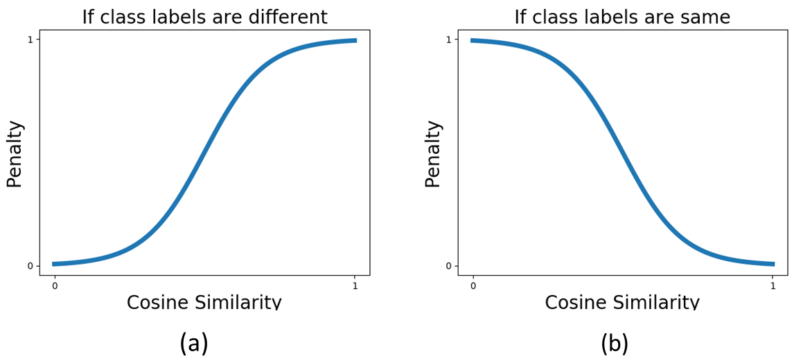
It is intuitive as to why samples belonging to case 1 can be difficult. For case 2, while one can expect semantic dissimilarity between a class, we look at the extreme cases, where the samples even though are part of the same class, could be referring to two different concepts within the same class. For a given sample $e_{i}$, we consider its pairwise relationship (PR) with all other samples in the dataset to compute its overall difficulty score. However, the intention is to only penalise the sample pair if it meets the above criterion (case 1&2). Thus, we introduce penalty functions (see Figure 1) that consider the PR and corresponding labels to output a penalty score for the input pair $(e_{i}$, $e_{j})$.

For a sample pair $(e_{i}$, $e_{j})$, the PR is captured by the cosine similarity $cos(e_{i},e_{j})=\frac{e_{i}\cdot e_{j}}{||e_{i}||||e_{j}||}$. Instead of determining a threshold on the $cos_{sim}$ to identify if the samples are similar or dissimilar, we employ a sigmoid function to assign the penalty scores. Specifically, we use an s-shaped sigmoid $S(x)=\frac{1}{1+e^{(a-bx)}}$ for case 1 and a z-shaped sigmoid $Z(x)=\frac{1}{1+e^{-(a-bx)}}$ for case 2 where $a,b>0$ and $x$ is the $cos_{sim}$. Thus, if the samples belong to different classes but have a high $cos_{sim}$, utilizing $S(x)$, a high penalty value is assigned and vice-versa. Similarly, if the samples belong to the same class but have high $cos_{sim}$, utilizing $Z(x)$, a low penalty value is assigned and vice-versa.

For each sample in the dataset, a cumulative penalty score is computed by summing the pairwise penalty scores with all the other samples in the dataset. The samples in the dataset are sorted in descending order w.r.t. the cumulative penalty scores and the top $k\%$ samples are labelled as difficult. The overall approach is summarized in Algorithm 1.

We identify 13 standard datasets used for text classification from prior art literature as shown in Table 2 and use the standard split for train, validation, and test sets when available. For AT Rane and Kumar 2018, MR Pang et al. 2002a and SE Nakov et al. 2019 a 10% split from training set has been used as a validation set.

As seen from the results shown in Table 2, an improvement in the F1 scores (upto $\sim$9%) is seen for most of the datasets. The values for $F1_{Best}$ indicate that the improvement is generally observed for $k\in[1,3,5]$. Although we saw a consistent improvement in the performance of the trained models on the updated train set (difficult samples removed) for lower values of $k$, we observed a consistent drop in performance when top 10% or 20% difficult samples were removed. This suggests that the top-ranked difficult samples in the training set ($k\in[1,3,5]$) help in model generalization while for $k>5$ the trained models seem to overfit on the training set resulting in poor performance on the test set. The CM dataset Collins et al. 2018 is an exception to this general trend. On further investigation, we observed that the top ranked difficult samples belong to a minority class and removing them hurts the model performance for test samples from that class. Thus, for text datasets, we observe that semantically difficult samples pose a challenge for the downstream model and removing them in most cases improves its performance.

Figure 2 shows the various regions in the TSNE plots corresponding to the top-ranked difficult samples belonging to various cases as discussed in Sec 2.1. The difficult samples due to case 1 (Figure 2(c)) belong to the region of maximum overlap between the class distributions. On the contrary, difficult samples due to case 2 (Figure 2(d)) belong to isolated clusters of samples that are not representative of the respective overall class distributions. Figure 2(b) shows the region of difficult samples when both cases are considered for YTS dataset. Figure 3 shows the trend of the F1 scores for all three cases. As observed, the performance gain is higher when difficult samples from both cases are considered than difficult samples from only case 1 or case 2 for $k\in[1,3,5]$, while for $k>5$, the performance dips for all configurations.

Table 3 showcases a few examples of top-ranked difficult samples identified from YTS dataset. As seen from examples of Spam class, the constituent words are common with the Not Spam class and the overall semantic meaning does not specifically indicate the label Spam. These particular samples lie in the overlap region as shown in Figure 2(b) and removing them from the training set improves the generalizability of the trained model. Similar insights can be derived for the difficult samples belonging to Not Spam class.

Table 4 shows the F1 scores obtained after removing difficult samples identified using Word2Vec embeddings and SVM classifier as discussed in Sec 3.2. We observe a similar improvement in the model performance after removing the top 1% difficult samples as shown in Table 2. We replicated the experiments to use TF-IDF Sammut and Webb 2010 as well as Fasttext Bojanowski et al. 2017 embeddings and observed a similar trend. Thus, the identification of difficult samples is agnostic to the underlying text encoding scheme and improves the performance of general text classification model.

Difficult samples in a dataset could arise due to the data gathering process which might induce noisy labels. It can also be an intrinsic property of the dataset where gathered labels are not sufficient to capture the overall set of semantic topics and fine-grained labels are necessary. As seen from our analysis, the difficult samples are most likely to get misclassified by the trained model. Thus, our approach can quickly identify the semantically difficult samples in a dataset which a data scientist could use to review their labels with the help of a domain expert or build provisions in the modeling pipeline to address them.

References

- Adi and Çelebi (2014) Abdulwahab O Adi and Erbuğ Çelebi. 2014. Classification of 20 news group with naïve bayes classifier. In 2014 22nd Signal Processing and Communications Applications Conference (SIU), pages 2150–2153. IEEE.
- Alberto et al. (2015) Túlio C Alberto, Johannes V Lochter, and Tiago A Almeida. 2015. Tubespam: Comment spam filtering on youtube. In 2015 IEEE 14th international conference on machine learning and applications (ICMLA), pages 138–143. IEEE.
- Almeida et al. (2011) Tiago A Almeida, José María G Hidalgo, and Akebo Yamakami. 2011. Contributions to the study of sms spam filtering: new collection and results. In Proceedings of the 11th ACM symposium on Document engineering, pages 259–262.
- Bojanowski et al. (2017) Piotr Bojanowski, Edouard Grave, Armand Joulin, and Tomas Mikolov. 2017. Enriching word vectors with subword information.
- Collins et al. (2018) Edward Collins, Nikolai Rozanov, and Bingbing Zhang. 2018. Evolutionary data measures: Understanding the difficulty of text classification tasks. arXiv preprint arXiv:1811.01910.
- Csáky et al. (2019) Richárd Csáky, Patrik Purgai, and Gábor Recski. 2019. Improving neural conversational models with entropy-based data filtering. In Proceedings of the 57th Annual Meeting of the Association for Computational Linguistics, pages 5650–5669.
- Davidson et al. (2017) Thomas Davidson, Dana Warmsley, Michael Macy, and Ingmar Weber. 2017. Automated hate speech detection and the problem of offensive language. In Proceedings of the International AAAI Conference on Web and Social Media, volume 11.
- Ghorbani and Zou (2019) Amirata Ghorbani and James Zou. 2019. Data shapley: Equitable valuation of data for machine learning.
- Hochreiter and Schmidhuber (1997) Sepp Hochreiter and Jürgen Schmidhuber. 1997. Long short-term memory. Neural computation, 9(8):1735–1780.
- Jain et al. (2020) Abhinav Jain, Hima Patel, Lokesh Nagalapatti, Nitin Gupta, Sameep Mehta, Shanmukha Guttula, Shashank Mujumdar, Shazia Afzal, Ruhi Sharma Mittal, and Vitobha Munigala. 2020. Overview and importance of data quality for machine learning tasks. In Proceedings of the 26th ACM SIGKDD International Conference on Knowledge Discovery & Data Mining, pages 3561–3562.
- Kotzias et al. (2015) Dimitrios Kotzias, Misha Denil, Nando De Freitas, and Padhraic Smyth. 2015. From group to individual labels using deep features. In Proceedings of the 21th ACM SIGKDD International Conference on Knowledge Discovery and Data Mining, pages 597–606.
- Li and Roth (2002) Xin Li and Dan Roth. 2002. Learning question classifiers. In COLING 2002: The 19th International Conference on Computational Linguistics.
- Mikolov et al. (2013) Tomas Mikolov, Kai Chen, Greg Corrado, and Jeffrey Dean. 2013. Efficient estimation of word representations in vector space. arXiv preprint arXiv:1301.3781.
- Nakov et al. (2019) Preslav Nakov, Alan Ritter, Sara Rosenthal, Fabrizio Sebastiani, and Veselin Stoyanov. 2019. Semeval-2016 task 4: Sentiment analysis in twitter. arXiv preprint arXiv:1912.01973.
- Pang et al. (2002a) Bo Pang, Lillian Lee, and Shivakumar Vaithyanathan. 2002a. Thumbs up? sentiment classification using machine learning techniques. arXiv preprint cs/0205070.
- Pang et al. (2002b) Bo Pang, Lillian Lee, and Shivakumar Vaithyanathan. 2002b. Thumbs up? sentiment classification using machine learning techniques. In Proceedings of the 2002 Conference on Empirical Methods in Natural Language Processing (EMNLP).
- Peinelt et al. (2019) Nicole Peinelt, Maria Liakata, and Dong Nguyen. 2019. Aiming beyond the obvious: Identifying non-obvious cases in semantic similarity datasets. In Proceedings of the 57th Annual Meeting of the Association for Computational Linguistics, pages 2792–2798.
- Rane and Kumar (2018) Ankita Rane and Anand Kumar. 2018. Sentiment classification system of twitter data for us airline service analysis. In 2018 IEEE 42nd Annual Computer Software and Applications Conference (COMPSAC), volume 1, pages 769–773. IEEE.
- Sammut and Webb (2010) Claude Sammut and Geoffrey I. Webb, editors. 2010. TF–IDF, pages 986–987. Springer US, Boston, MA.
- Swayamdipta et al. (2020) Swabha Swayamdipta, Roy Schwartz, Nicholas Lourie, Yizhong Wang, Hannaneh Hajishirzi, Noah A Smith, and Yejin Choi. 2020. Dataset cartography: Mapping and diagnosing datasets with training dynamics. In Proceedings of the 2020 Conference on Empirical Methods in Natural Language Processing (EMNLP), pages 9275–9293.
- Uzzi et al. (2016) Brian Uzzi, Lise Getoor, Evimaria Terzi, and Lada Adamic. 2016. Four keynote speeches [2016 ieee/acm international conference on advances in social networks analysis and mining]. In 2016 IEEE/ACM International Conference on Advances in Social Networks Analysis and Mining (ASONAM), pages xl–xliii. IEEE Computer Society.
- Yoon et al. (2020) Jinsung Yoon, Sercan Arik, and Tomas Pfister. 2020. Data valuation using reinforcement learning. In International Conference on Machine Learning, pages 10842–10851. PMLR.