Stanford University and https://sites.google.com/view/mohakgmohakg@stanford.eduhttps://orcid.org/0000-0002-1176-5549 Stanford University and https://sukolsak.com/sukolsak@gmail.com Stanford University and https://sahasrajit123.github.io/sahasras@stanford.eduhttps://orcid.org/0000-0002-6652-4881 Stanford University and https://web.stanford.edu/~ashishg/ashishg@stanford.edu
Low Sample Complexity Participatory Budgeting
Abstract
We study low sample complexity mechanisms in participatory budgeting (PB), where each voter votes for a preferred allocation of funds to various projects, subject to project costs and total spending constraints. We analyse the distortion that PB mechanisms introduce relative to the minimum-social-cost outcome in expectation. The Random Dictator mechanism for this problem obtains a distortion of . In a special case where every voter votes for exactly one project, [11] obtain a distortion of We show that when PB outcomes are determined as any convex combination of the votes of two voters, the distortion is . When three uniformly randomly sampled votes are used, we give a PB mechanism that obtains a distortion of at most thus breaking the barrier of with the smallest possible sample complexity.
We give a randomized Nash bargaining scheme where two uniformly randomly chosen voters bargain with the disagreement point as the vote of a voter chosen uniformly at random. This mechanism has a distortion of at most 1.66. We provide a lower bound of 1.38 for the distortion of this scheme. Further, we show that PB mechanisms that output a median of the votes of three voters chosen uniformly at random, have a distortion of at most 1.80.
ccs
Applied computingkeywords
Social Choice, Participatory budgeting, Nash bargaining1 Introduction
More than 1500 cities around the globe have begun adopting Participatory Budgeting (PB) [22, 13], a process through which residents can vote directly on a city government’s use of public funds. Residents might, for example, vote directly on how to allocate a budget of reserved funds between projects like street repairs or library renovations. PB has been shown to promote government transparency, resident engagement, and good governance [23].
We study a PB setup similar to [12] where each vote is an allocation of funds to projects (we call it a “preferred budget”) subject to the constraint that the sum of allocations to all projects is equal to one. Projects have a fixed cost, and allocations to any project cannot exceed its cost. However, allocations less than the project’s cost are allowed. ([12] consider all project costs equal to one). In this model, therefore, every vote and the outcome of the PB election can be represented as a point on the unit simplex.
We study the distortion (Definition 5) that PB mechanisms introduce in expectation relative to the social cost minimizing allocation in the worst case of PB instances, following the lines of [1]. We adopt the distance as the cost function where a voter with preferred budget experiences a cost of from an outcome budget (Definition 2).
Several preference elicitation methods have been studied for PB [7, 2, 15, 5]. Policymakers must then transform a list of votes into a real-world allocation of funds. Furthermore, even though there may be an “optimal” allocation (under natural notions of social welfare), this allocation may be intractable to compute [18, 20] or difficult to reliably estimate if turnout is low [8]. In some situations, policymakers need to obtain a quick estimate of the budgetary region in which preferences may lie. In these cases, and when running a fully-fledged PB election is costly or difficult, low-sample complexity PB mechanisms are an attractive choice.
Low-sample complexity preference elicitation mechanisms have also been of interest recently in computational social choice [11, 10, 1, 9] – in this work, we give low-sample complexity mechanisms (using the preferred budgets of a small number of sampled voters) for PB, which achieve a distortion of less than 2. Note that is a natural barrier for the distortion in this problem since the Random Dictator mechanism achieves a distortion of 2 in our model of PB. The Random Dictator mechanism chooses the outcome as the preferred budget of a uniformly randomly chosen voter. From Theorem 5 of [1], its distortion is at most , and from our Lemma 7, it is . We further prove that a mechanism that chooses any linear combination of two randomly sampled votes (Random Diarchy) also attains a distortion of 2 (Lemma 8). Another low sample-complexity mechanism, Random Referee [10], asks a randomly chosen voter (“the referee”) to choose one out of two possible outcomes, which are random samples from the preferred budgets of the voters. This mechanism also attains a distortion of at least 2 in our setup (Lemma 9). We give a PB mechanism which samples three voters uniformly at random and attains a distortion of at most 1.66.
1.1 Our Contributions
When the PB mechanism samples three voters uniformly at random, we show that aggregation schemes that choose a median of their preferred budgets achieve a distortion of at most 1.80. We refer to such schemes as the median schemes and denote this class of schemes by .
We then turn to the case where two uniformly randomly chosen voters can come together and “bargain” with a third voter’s preferred budget (again chosen uniformly at random) as the “disagreement point.” We formulate the bargaining rules for the voters via the well-studied Nash bargaining framework [6]. When these bargaining rules can be further specified by a randomized rule (§4.2), we show that the distortion of the resulting mechanism is at most (Theorem 35). We call this mechanism the randomized Nash bargaining scheme .
A key technical tool we use is the analysis of pessimistic distortion (PD) (Definition 26) first proposed by [10]. PD is a form of distortion where the comparison is made with a counterfactual which chooses a separate outcome for every small subset of voters (of a fixed size ), thereby attaining a lower social cost than the true ‘optimal’. In this work, we use . This choice is due to computational constraints. We show that the PD with is an upper bound on the distortion of our proposed mechanisms with any number of voters .
We then reduce the problem of computing the PD into a set of linear programs for the median schemes and bilinear programs of constant size for the randomized Nash bargaining scheme . For this, we use a projection of the preferred budgets of voters into a space (we call it the incremental allocation space (§3)) that captures the common preferences of a subset of voters relative to other voters. In the median schemes, funds are allocated to projects ensuring that the final outcome is the median of the preferred budgets of three randomly sampled voters. In the randomized Nash bargaining scheme , the expected funds allocated to a project satisfy additional proportionality constraints (§4.2), resulting in bilinear programs. Since the proportionality constant is not fixed, this results in another variable in the optimization formulation. The problem has a complex combinatorial structure due to the nuances of Nash bargaining. However, we are able to exploit symmetries of the problem, enabling us to solve it efficiently. Since the bilinear programs are of a constant size (depends on , which we set to ), we can solve these in fixed time.
Same as Random Dictator and Random Referee, our PB mechanism also naturally respects project interactions such as complementarity and substitution as long as the voters are aware of these interactions. This is because the bargaining outcome between two voters is guaranteed to be Pareto optimal for them. We describe this point in detail in §8.
1.2 Related Work
The sequential deliberation (SD) mechanism for social choice was proposed in [11] where the two uniformly randomly chosen voters deliberate in each round under the rules of Nash bargaining, and the outcome for every round is the disagreement point for the next round. The SD for one round corresponds to the randomized Nash bargaining scheme . They analyzed the mechanism in median spaces, which include median graphs and trees, and found an upper bound of the distortion of the mechanism to be 1.208. They also analyze the distortion in the budget space (or unit simplex) in a special setting where each voter only approved funds for a single project. In this case, they show that the distortion in the equilibrium of SD is . This paper extends their work in the case of the unit simplex, such that voters in our model do not have to restrict their vote to one project.
The authors of [16] study a model where voters’ opinions evolve via deliberations in small groups over multiple rounds. Opinions in their model correspond to preferred budgets in our model; however, unlike preferred budgets, opinions change as a result of deliberations. They study the distortion in single-winner elections setting and show that it is bounded by when voters deliberate in groups of ( is the number of voters).
The work most closely related to ours is [10]; they study the random referee mechanism. We use their technique of analyzing the PD of 6 voters. However, they apply this technique where the underlying decision space is the Euclidean plane and use the underlying geometric structure to perform a grid search. In contrast, we study the PD with Nash bargaining, which leads to a complex structure of outcomes that we capture in linear or bilinear programs.
The authors of [9] analyze low sample-complexity randomized mechanisms for PB. They obtain constant factor guarantees for higher moments of distortion, and the distortion bound they provide is much larger than 2. Several additional results and research directions in PB are described in the survey [4].
1.3 Future Directions
A natural direction for future work is to analyze the distortion for multiple rounds of deliberation in our model, with every round’s outcome serving as the next round’s disagreement point. Another interesting modelling question is to study the deliberation or bargaining process with more than two agents participating together. Closing the gap of the distortion of also remains an interesting open problem.
1.4 Roadmap
We describe the model and preliminaries in §2, introduce a projection operation and give some technical results in §3, characterize the outcome of different schemes in §4. We derive the distortion of the class of median schemes in §5. We derive the distortion under in §6. We give empirical results on real-world Participatory Budget (PB) data in §7, and discuss project interactions in §8.
2 Model and Preliminaries
Suppose we have projects and are required to design a budget. A budget denotes the fraction of the total funds that are to be spent on each project. Projects have a maximum possible allocation or “project costs.” All votes respect these project costs, and consequently, the outcomes of all our mechanisms also respect the project costs.11 1 There is no constraint on the minimum allocation to a project other than that it must be non-negative. For notational simplicity, we drop the project costs from the model henceforth and operate under the assumption that project costs are . All our results trivially follow for general project costs.
Definition 1.
Let denote the funds allotted to project in budget . We define the budget simplex as the set of valid budgets i.e., = .
There are voters, each with a preferred budget A vote profile denotes the list of preferred budgets of all voters, i.e, . The funds allotted to project by voter is A vote profile defines an instance of PB. The outcome of an instance of PB is a budget in Voters adopt the distance as the cost function. (Not to be confused with the project costs, which is a different concept here.)
Definition 2.
For the cost of an outcome for a voter with preferred budget is The sum of cost over all budgets, is the social-cost of budget .
We define the overlap utility which is closely related to the cost. Note that this notion of overlap utility has been studied in knapsack voting [15, 12].
Definition 3 (Overlap Utility).
Lemma 4.
For budgets , .
A proof is in Appendix A.13. Lemma 4 implies that for a voter, maximizing overlap utility is the same as minimizing the cost. Note that overlap utility is symmetric, i.e,
2.1 Distortion
Here we define distortion, which we use as a metric to quantify how good a outcome is in comparison to the optimal solution for minimizing social-cost. We define distortion through the cost .
Definition 5.
The distortion of budget for vote profile is
Let be the output of mechanism for vote profile .
Definition 6.
The distortion of a class of voting mechanisms is:
Note that distortion is defined as a supremum over all instances of PB and all mechanisms in class 22 2 We will often study the distortion of a single mechanism, i.e., not a class. In that case, simply denotes the distortion of the mechanism . The expectation is over the randomness of the mechanism, which also includes the randomness in the selection of voters.
The distortion of a voting mechanism is widely used to evaluate its performance regarding how close its output is to the social cost-minimizing outcome in expectation [1, 19, 3, 14, 10]. The Random Dictator [1] voting mechanism has a distortion of as shown in Lemma 7. A proof is given in Appendix A.1.
Lemma 7.
Any aggregation method constrained to choose its outcome as the preferred budget of a uniformly randomly chosen voter has distortion .
Now, consider a mechanism that chooses the outcome via the deliberation between two voters chosen uniformly at random with preferred budgets and . Within this class, we consider mechanisms constrained to choose the outcome as a convex combination of budgets and .
Now, consider a mechanism constrained to choose the outcome as a linear combination of budgets and where and denote the preferred budgets of randomly sampled voters. That is, for Note that may be optimized over the entire vote profile.33 3 All such outcomes maximize the sum of the overlap utilities of the deliberating agents. We refer to this class of mechanisms as Random Diarchy and denote it by . Interestingly, the distortion of is 2, the same as that of Random Dictator.
Lemma 8.
For Random Diarchy
A proof is given in Appendix A.2. We further show that Random Referee scheme described in [11] where one of the two preferred budgets of the bargaining voters is chosen based on the preferred budget of third sampled voter also has a distortion ratio of at least 2 in Lemma 9, proven in Appendix A.3. We denote the class of such mechanisms by .
Lemma 9.
For Random Referee
2.2 Model of preference aggregation
Let us define the mechanism formally in steps and we call it Triadic scheme.
- 1.
Pick a voter uniformly at random and set the disagreement point as the preferred budget of voter .
- 2.
Now choose two voters and uniformly at random with replacement and they bargain with as the disagreement point.
All our theoretical results in this paper are for the outcome of the triadic scheme. However, as discussed in [11], we can extend this bargaining scheme to multiple rounds by setting the outcome of the previous round as the disagreement point for the next round and sampling the two bargaining voters uniformly at random without replacement. We provide empirical results for this setup for multiple rounds (upto 10 rounds) in § 7.
Our bound on pessimistic distortion assumes that the voters are chosen with replacement as done in [10]. This directly gives us a bound on the distortion when voters are sampled without replacement. It is easy to see that the difference in these bounds is of The case where two or more identical voters are sampled out of three defaults to the Random Dictator mechanism, which has constant distortion – the probability of this event is of .
We consider bargaining schemes satisfying one or more of the following constraints, namely a) Pareto efficiency, b) Invariance to Affine Transformation, c) Symmetry, and d) Independence of Irrelevant Alternatives. Bargaining schemes that satisfy all of these constraints are the class of Nash bargaining schemes denoted by [6].
Definition 10.
An outcome of , the Nash bargaining between two voters with preferred budgets and and the disagreement point , is a budget which maximizes the Nash product , subject to individual rationality and , and in case of a tie between possible outcomes, maximizes .
The fact that breaks ties in favor of the disagreement point is crucial for the distortion of triadic scheme with bargaining schemes in to be smaller than . It is also crucial for the membership of in a class of bargaining schemes that maximize the sum of overlap utilities of the bargaining agents and the disagreement point. We now define this class of bargaining schemes.
Definition 11.
is the class of median schemes if any outcome maximises the sum of utilities with budgets and i.e. .
The following important result is proved in Appendix A.11.
Theorem 12.
Every scheme in is also a median scheme i.e.
3 Incremental allocation space
We now give a function that captures the marginal preferences of a subset of voters regarding the allocation to project , relative to the preference of the other voters (i.e., ). This function will be useful as an analytical tool in the paper. Specifically,
Definition 13.
Given a vote profile and project the incremental project allocation maps a subset of budgets to
Here and over are defined as 0 and 1, respectively. denotes the amount by which the budgets in all agree on increasing the allocation to project above the maximum allocation to by any budget in . Summing this quantity over all projects gives us which is defined in the following.
Definition 14.
For a vote profile the incremental allocation is for all
We use in §5 since its complexity is dependent only on the number of voters and not on the number of projects . This helps us give results valid for arbitrarily large values of . We illustrate the functions and in the following example.
Example 15.
Consider an instance of PB with three projects and a vote profile with three budgets , , and . 44 4 For brevity, we omit braces and commas in the argument of . Then, This is because the budget has allocation to project out of which only is incremental on top of . Also, As a result, Similarly Also, . Further, . This is because the subset has a minimum allocation of to project among themselves. It is also incremental since . Further, we have This is because the group of all three budgets has no allocation that is common to all. Finally, because no budget allocated funds more than 0.5 to project 3.
We use to denote the power set of . We now give an important corollary regarding the function .
Corollary 16.
A proof is given in Appendix A.8. Corollary 16 says that every incremental allocation to project by budgets in adds up to 1 when summed over all subsets (this includes the empty set; implies that no voter allocated the full 1 unit budget to project ).
3.1 Projection On Incremental Allocations
We now give a projection of from to to get This operation has two applications in this paper. First, it enables us to study the allocations of an outcome relative to the vote profile by making projections from to Second, it is used to study the outcomes of bargaining with a subset of voters with respect to the entire vote profile via projections from to .
Lemma 17.
For any vote profile and , the projection from to is for all and all . Summing over ,
A proof is given in Appendix 17. Lemma 17 captures an important technical fact. To calculate the incremental project allocation function on over a vote profile , i.e., , we may sum over all subsets of budgets in which contain all elements of but no element of . Note that here
We now consider the problem of analyzing an outcome with the help of the incremental allocation function. Towards this, we define the function with respect to an outcome with the help of the projection operation described in Lemma 17.
Definition 18.
For vote profile and budget , define as
Recall from Definition 13 that denotes the amount by which all budgets in want to increase the allocation to project over the maximum allocation to by any budget in The quantity denotes the amount by which the outcome budget “accepts” this preference of . Naturally,
Analogous to summing over all to get we can sum over all to get .
Definition 19.
For vote profile and budget , define as
informally denotes the amount by which outcome budget “accepts” the preference of for increasing allocations above the allocations of across all projects. See that
Corollary 20.
For any vote profile P and budget , for all Summing over , .
Proof.
Follows directly from Lemma 17 since (we are projecting from to ). ∎
Corollary 21.
for all vote profiles and Summing over all projects , we get
This result captures, in the incremental common budget space, the fact that the total funds allocated by a budget to projects is 1. The following example illustrates .
Example 22.
Consider vote profile with two projects. Let the budgets and be and respectively. Let the outcome budget be . In this case, and since the excess allocation by outcome to project over the allocation by budget (i.e., 0.4) is larger than the least excess allocation to project by budgets and over allocation in budget (i.e., which is 0.3). In other words, the entire incremental allocation to project 2 by budgets and is accepted by outcome . However, but since the incremental allocation to project by budget over budgets and is 0.1. Thus only a partial incremental allocation to project by budget is ”accepted” by budget .
4 Overview of Median and Nash bargaining schemes
Recall the triadic mechanism from § 2.2 and we characterize its outcome. Let the disagreement point be and the preferred budgets of the agents chosen randomly for the mechanism be and . For simplicity of notation, we denote by for being any subset of 55 5 Note that we do not consider in this section where is the set of the preferred budgets of all the voters, even those not involved in the bargaining.. We also denote the outcome budget of the bargaining by and by for .

4.1 Overview of class of schemes and
In Figure 1, we illustrate the incremental allocations with budgets and on a Venn diagram. Recall from Definition 19 that denotes what incremental allocation from is ”accepted” by outcome . For the construction of , the bargaining agents first select all the allocations ”agreed” to by at least two of the three budgets. In Figure 1, this corresponds to the area of the overlaps. Now, we have two cases, i.e. the total allocation to is less than 1 or exceeds 1. We denote the difference between 1 and the total allocation to by Excess.
Consider the case when the total allocation to is less than 1. Here, the agents need to make further allocations worth Under the class of median schemes [described in §4.3], they may select project allocations from and arbitrarily into the outcome and thus into and . In Figure 1, this corresponds to the area covered by exactly one of the budgets. However, under Nash bargaining schemes , they select allocations worth from each of and
Now, consider the case when the total allocation to is more than 1. In this case, under median schemes, , the participating agents select total project allocations worth Excess arbitrarily from and and remove allocations to these projects. In Figure 1, this corresponds to the area of the overlap of exactly two budgets. However, under Nash bargaining schemes , they select allocations worth from each of and and remove allocations to these projects from the outcome .
The following lemma characterizes the overlap of the outcome with the budgets , and , in terms of the incremental allocation functions and .
Lemma 23.
For any preferred budgets of bargaining agents and , disagreement point , and outcome of ,
Where,
Proof Sketch.
In Nash bargaining, no part of is such that it is not preferred by both and . That is, . Otherwise, we could construct a new outcome that reallocated the funds from or to and . This would increase and and thus would not be Pareto optimal. The parts of that benefit both and must be maximized. That is, and . Otherwise, we could construct a new outcome that reallocates funds from any other project to the project that benefits both and , thus showing that is not Pareto optimal. The remaining part of the proof is technical and is in Appendix A.12. ∎
We give an explanation of the construction of the Nash bargaining solution (and correspondingly ) in three steps.66 6 The steps are only for illustration purposes. There is no chronology or structure required in bargaining processes. We can only characterize the outcome.
Step 1: The voters with preferred budgets and mutually decide to allocate funds to projects that benefit both of them. This means, for all projects In terms of and this corresponds to and At this point, is zero for all other subsets of
Step 2: At this point, the total allocation to projects in the bargaining outcome may be less than 1. The bargaining agents now allocate more funds to the projects for which and Now is set to the “median” of for all projects In terms of and this corresponds to setting and
Step 3: Now, two possibilities arise for the total amount of funds allocated in so far, i.e., the bargaining agents have either over-spent or under-spent the total funds. These cases are central to the analysis in the paper and will be revisited several times.
Case 1: The total funds currently allocated in is at most 1, i.e., This is same as:
| (1) |
Recall the definition of Excess in Lemma 23. In this case, since there is a positive the bargaining agents now allocate more funds to projects with . Since in Nash bargaining we assume equal importance of the overlap utilities of both the bargaining agents, they divide the Excess equally. They incrementally fund projects with and the projects with with amount each. They ensure that The precise manner of doing so is not important to satisfy the axioms of Nash bargaining. In terms of this corresponds to setting .
Case 2: The total funds currently allocated in exceeds 1, i.e., This is same as:
| (2) |
If we are in this case, then the bargaining agents have overspent the funds and Excess is negative. They need to remove amount of allocations from . Recall that at this point, is set to the median of for all projects They remove funds from projects with and the projects with with amount each. They ensure that The precise manner of doing so is not important to satisfy the axioms of Nash bargaining. In terms of this corresponds to setting and
We now give a randomized way of allocating the Excess funds in 4.1 while satisfying the axioms of Nash bargaining.
4.2 Randomised Nash bargaining solution
4.1: Denote for all projects .77 7 This precisely corresponds to in the incremental allocation space. To projects with , allocate incremental funds at random such that is proportional to The sum of over all is and no incremental allocation is more than .88 8 The randomness of this process is the same as the hypergeometric distribution with (discretized) balls corresponding to each project in an urn, and we pick (discretized) balls without replacement to provide incremental allocations. A similar process is followed for projects with by defining and making incremental allocations summing to , proportional to and with
4.1: Denote for all projects .99 9 This precisely corresponds to in the incremental allocation space. From projects with , remove amount of previously allocated funds at random such that is proportional to The sum of over all is and with . A similar process is followed for projects with by defining and removing allocations from project summing to , proportional to and with
4.3 Median schemes
Theorem 24.
The proof of this theorem is technical and is given in Appendix A.10.
Note that all the conditions on the outcomes of the bargaining schemes in are symmetric in all three of . However, outcomes in also satisfy some additional conditions which may not be symmetric in all three of .
We now give a lower bound on Since contains , this bound also applies to Moreover, the same bound also holds for the distortion of
Theorem 25.
Also,
Proof.
The proof is by the following example of a PB instance. Suppose there are voters and projects for some . Let denote the budget where the -th project receives allocation and all the other projects get allocation . Each voter in group A prefers budget . Each voter in group B ) prefers budget . The analysis of this example is in Appendix A.4. where we set ; ∎
We now give upper bounds of the distortion of .
5 Distortion Of Schemes in
To find an upper bound of the distortion of triadic scheme with any bargaining scheme, we use a technique introduced in [10], called pessimistic distortion (PD). In this technique, we first analyze the distortion for a small group of voters, call it PD, and then show that the distortion over all voters cannot be more than the PD. Specifically, in this paper, we analyze the PD for a group of voters. The idea is that we allow the counterfactual solution to choose a separate ‘optimal’ budget for every -tuple of voters, thereby attaining a smaller social cost than a common outcome for all voters. On the other hand, for our mechanism, we consider the expected social cost under one outcome. This is why the distortion calculated is pessimistic. Formally:
Definition 26.
The pessimistic distortion (PD) of the class of mechanisms with triadic scheme with 6 voters is:
Here denotes the set of all -combinations of set .1010 10 For simplicity of notation, we use in place of in PD.
Notice that in the definition of PD, we only consider the cost for the non-bargaining agents (same as in [10]). We illustrate the PD in Figure 2, where the bargaining is over budgets the disagreement point is and the cost is computed only for the budgets not involved in the bargaining. This definition is more pessimistic than considering all agents’ costs. Further, since the outcome of is 4.3 in we can use any combination of three voters to compute the outcome of bargaining without designating one of the budgets as the disagreement point.

The next result, proved in Appendix A.14 , is that the distortion of any bargaining scheme in with triadic scheme cannot be more than its PD with triadic scheme with only voters.
Lemma 27.
.
We now give a representation of the overlap utilities (equivalently the cost ), in terms of the incremental allocations . This representation is of technical importance for proofs.
Lemma 28.
For budgets and a vote profile that includes , we have .
Proof.
Lemma 28 shows that the overlap utility between two budgets is the same as the sum of what , and all subsets of the other budgets in have in common via the incremental allocation function . For example, if then
Lemma 28 is useful for the proof of the following important result, which is an upper bound for
Lemma 29.
.
We give a sketch of the proof here. The detailed proof is in Appendix A.15.
Proof Sketch.
Let denote a budget obtained on bargaining with budgets in set using a bargaining scheme in . Note that mechanisms in are 4.3 in therefore, we do not need to designate a disagreement point in for analysis.
Suppose that . Then the following optimization problem has an optimal objective value strictly greater than .
| maximize | ||||
| subject to | ||||
| (3) |
To convert this problem into a linear program, we map it to the incremental allocation space of the set of 6 budgets . Denote by for simplicity of notation in the optimization programs. Similar to Definition 19, we define via the ‘optimal’ budget and using the outcome of our mechanism , for each .
By Lemma 4, we write the cost in terms of the overlap utility which, by Lemma 28 and the definition of , equals . Similarly, we have To make the constraints linear, we use case analysis.
Consider a given and a budget . Let and . Theorem 24 implies that if and only if the following holds:
We break each constraint into two cases. Since there are such constraints in the optimization problem, there are cases overall. We represent each case by a binary string of length 20 where a 0 or 1 at each position denotes whether the triplet corresponding to that position is in 4.1 or 4.1.
However, most of these cases are not unique up to the permutation of preferred budgets, i.e. when the preferred budgets of different voters are permuted, we may move from one case to another. Since these cases have the same objective value, we do not need to solve all the cases. Exploiting further symmetries, we have 2136 unique cases, each of which is formulated as a linear program with precise details in Appendix A.15. We obtain the optimal value for each case to be 0 hence, a contradiction. ∎
Theorem 30.
.
6 Distortion of
Recall the randomized Nash bargaining scheme explained in § 4.2. In this section, we derive an upper bound for it. Towards this, we first define a hypothetical bargaining scheme This scheme is hypothetical because it assumes that the bargaining agents use some knowledge about the preferred budgets of the non-bargaining agents to break ties among potential outcomes. We then show in Lemma 32 that the Distortion of is at most as much as that of We then bound the Distortion of by its expected pessimistic distortion (EPD), a quantity similar in essence to the PD. We define the EPD in Definition 33. Our main technical contribution in this section is the analysis of the EPD of , which we do by expressing it as the solution of a bilinear optimization problem.
6.1 Construction of bargaining solution in
Recall Definition 18 of for an outcome budget . Also recall that satisfies Corollaries 20 and 21. For we characterize the outcome in the incremental allocation space; denoted by Same as also satisfies Corollaries 20 and 21, i.e.,
| (4) | ||||
| (5) |
Before describing the construction of , we now give the following result on the overlap utility of outcome budget and any budget in terms of .
Lemma 31.
For a vote profile a budget and any budget , the overlap utility is
Proof.
In Lemma 28, use for , for and for . ∎
By Lemma 31, 1111 11 Note the overload in the notation of the overlap utility; it was initially defined for a pair of budgets and , here we define it for and where captures . Similarly, the cost can be given by
Let be the disagreement point, and be the preferred budgets of the agents chosen to bargain. Denote For the construction of we first do 4.1 and 4.1 from § 4. We then have for all for all such that contains at least 2 elements of and for all other . We then encounter either 4.1 or 4.1, as in § 4.
4.1: Here we need to allocate more funds to projects. Recall the construction of for in § 4.2. Recall the random incremental allocations and used in For the incremental allocations in we construct 1212 12 Note that since [follows from Lemma 17] and since [follows from Lemma 17] and the fact that [as defined in 4.1 in §4.2]. for all for all projects . Intuitively, this may be thought of as a proportional selection of projects from every subset of budgets . Similarly we construct for all and all projects
Now, set and and
4.1: In this case we need to remove allocations from projects. Recall the construction of for in § 4.2. Recall the removals of allocations and used in For the removals of allocations in we construct for all for all . Similarly we construct for all
Now, set and
We can now construct via With this, we now construct as the outcome of the hypothetical bargaining process, via the projection from to That is, [recall projection in Lemma 17].
6.2 Distortion under
We now bound the distortion of the triadic scheme with bargaining scheme by that of the hypothetical scheme . A proof is in the Appendix A.18.
Lemma 32.
.
We now follow a similar approach as in §5 and define expected pessimistic distortion under bargaining scheme as follows.
Definition 33.
The expected pessimistic distortion of with triadic scheme with 6 voters, is
Lemma 34.
Lemma 35.
The proof is similar to that of Lemma 29 and is presented in Appendix A.25. We present the key ideas of the proof here.
Proof Sketch.
We show in Appendix A.20 that and for some variables . Here, and denote what fraction of allocation from the incremental allocation is “accepted” into . In our optimization problem formulation equation (32) in Appendix A.25 ,we use as variables of our optimization formulation, together with and therefore we obtain a bilinear program. We solve it with the Gurobi solver [17]. Similar to the proof of Lemma 27, we remove the cases that are not unique to permutations of voters and use further symmetries of the problem to reduce number of bilinear programs from to 1244. ∎
Theorem 36.
7 Empirical Results
Recall triadic scheme as described in §2.2. We now define a sequential deliberation mechanism that could run bargaining over multiple rounds by setting the disagreement point for each round as the outcome of the previous round as proposed in [11].
- 1.
Pick a voter uniformly at random. Set the disagreement point for the deliberation to their preferred budget
- 2.
Repeat the following process times,
- (a)
Pick two voters independently and uniformly at random with replacement. They bargain with as the disagreement point.
- (b)
Set the disagreement point to the outcome of the bargaining.
- (a)
- 3.
The outcome of the process is .
Observe that on setting , we exactly get triadic scheme as §2.2. To evaluate the distortion of sequential deliberation in PB empirically, we ran a simulation from the online participatory budgeting elections in Boston in (), Cambridge in (), Greensboro in (), and Rochester in () where the data were obtained from https://budget.pbstanford.org/. In these elections, projects had a fixed cost, and voters participated in knapsack voting [15], in which they could choose any number of projects as long as they fitted within the fund limits. Note that in this simulation setup partial project funding is not allowed, unlike the setup in the theoretical model. We further present simulation results in Figures 4(a), 4(b), 4(c) on real dataset from a PB (participatory budgeting) process run by a non-profit organisation in Boston in 2016 where they used a fractional allocation setting, more aligned with our theoretical work.


To simulate sequential deliberation, we picked a voter uniformly at random to set their preferred budget as the disagreement point. We then picked another two voters independently and uniformly at random and calculated a Nash bargaining solution between them. We assumed that everyone voted truthfully. We then made the bargaining outcome the new disagreement point and repeated the deliberation process for rounds. We repeated this entire simulation times for each PB election. The average distortion after each round of deliberation is shown in Figure 3(a). The point corresponding to rounds of deliberation is the first disagreement point and is selected uniformly at random. Since voters did not have to use all the budget available, we added an ‘unspent’ project and allocated the unspent budget of each voter to this project. We normalized the budget to sum to in each election.
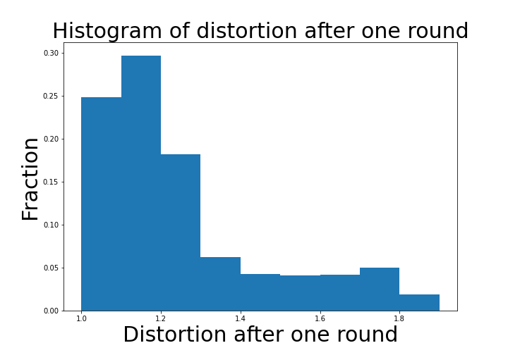
The mean and standard deviation of the distortion after each round of sequential deliberation for the fractional allocation setting as in the PB process in Boston is shown in Figures 4(b) and 4(c), respectively. A histogram plot of the distortion after one round of deliberation is in Figure 4(a). As before, we observe a quick convergence within three rounds of sequential deliberation with the point corresponding to zero rounds of deliberation being the first disagreement point.
The results from all the PB elections show that the average distortion is quite low, even after only two rounds of deliberation. It also shows that the distortion converges quickly within three rounds. Further, we measured the stability of the fund allocation to the projects after each round of deliberation. We simulated sequential deliberation on the data from the PB in Cambridge times, each time with rounds of deliberation. The fund allocation to each project after each round was recorded. The fund allocation’s standard deviation (SD) is shown in Figure 3(b). We can see that the SD stabilizes after only three rounds of deliberation.
8 Triadic Scheme With Project Interactions
Mathematically, we model project interactions as follows: if projects in group are perfect complements of each other, then the overlap utility that voters can derive from each project in is the minimum funding of any project in . For example, consider a proposal of buying some computers for the community. Within this, one project is for buying hardware and another one is for buying software. If the software and hardware projects are funded and then the community members can only use each, and the extra funding of for the hardware project is wasted 1313 13 This is a stylized model and in general, the scale of the funds required for each project can be very different..
On the other hand, if the projects in group are perfect substitutes, then the utility that voters can derive from group is the maximum funding of a project in . Thus, if two companies are paid and to do the same work, only will be used, and is wasted.
We now give a formal model of the set of projects. Let denote the number of groups of perfect complementary projects, denote the number of groups of perfect substitute projects, and denote the number of regular projects. Let denote the number of projects in group . For groups of perfect complementary and perfect substitute projects, and for regular projects The total number of projects is . For simplicity, project groups are arranged such that groups are perfect complementary, groups are perfect substitutes, and are regular projects.
Let be the efficiency function which quantifies how much budget respects the project interactions. Specifically, takes a budget and outputs a vector in , where
For a group of perfect complementary projects, the corresponding output element is the bottle-neck allocation in the group, multiplied by the number of projects in the group. For a group of perfect substitute projects, the corresponding output element is the largest allocation in that group. For regular projects, the corresponding output elements are the same as the allocation to the project. We now give a modified definition of the overlap utility, accounting for project interactions.
Definition 37.
The overlap utility of budgets and , accounting for project interactions is .
In the following definition we formally state the requirements for a budget to be consistent with the project interactions.
Definition 38.
A budget respects the project interactions if and only if projects in each perfect complementary group are all funded equally, and at most one project in each perfect substitute group is funded at all.
The following lemma states that the efficiency function sums to if and only if the budget respects the project interactions.
Lemma 39.
Budget respects the project interactions iff the efficiency function satisfies . Otherwise,
We now give a result that a Pareto improvement exists over a budget that does not respect the project interactions.
Lemma 40.
If , then for some , there exists a budget for which and for all project groups .
We now give the main result of this section. We show that if either of the budgets of the bargaining agents respect the project interactions (which will be true for rational agents), then the outcome of any median scheme respects project interactions. Since the class of median schemes contains the class of Nash bargaining schemes (Theorem 12), this result also applied to and therefore also to our randomized bargaining scheme
Theorem 41.
If budget or respects the project interactions, then for any budget respects the project interactions.
Proof.
Let be an outcome from . Assume without loss of generality that budget respects the project interactions, and suppose that outcome does not. By Lemma 39, and . Thus, there exists some where . By Lemma 40, there exists a budget which respects the project interactions and for all project groups and . The overlap utility functions satisfy:
This implies that the sum of overlap utilities of and with is higher than that with , a contradiction for an outcome of . ∎
Theorem 41 implies that if every voter has a preferred budget that respects the project interactions, then the outcome of the sequential deliberation mechanism will also respect the project interactions, no matter how many rounds it runs.
9 Conclusion
We study low sample-complexity mechanisms for PB, which are particularly attractive when the policymakers are interested in obtaining a quick estimate of the voter’s preferences or when a full-fledged PB election is difficult or costly to conduct. In our PB setup, the distortion of mechanisms that obtain and use the votes of only one uniformly randomly sampled voter is . Extending this result, we show that when two voters are sampled, and a convex combination of their votes is used by the mechanism, the distortion cannot be made smaller than . We then show that with samples, there is a significant improvement in the distortion – we give a PB mechanism that obtains a distortion of . Our mechanism builds on the existing works on Nash bargaining between two voters with a third voter’s preferred outcome as the disagreement point and give a lower bound of for our mechanism.
References
- [1] Elliot Anshelevich and John Postl. Randomized social choice functions under metric preferences. Journal of Artificial Intelligence Research, 58:797–827, 2017.
- [2] Kenneth J Arrow, Amartya Sen, and Kotaro Suzumura. Handbook of social choice and welfare, volume 2. Elsevier, 2010.
- [3] Haris Aziz, Bo Li, and Xiaowei Wu. Approximate and strategyproof maximin share allocation of chores with ordinal preferences. Mathematical Programming, pages 1–27, 2022.
- [4] Haris Aziz and Nisarg Shah. Participatory budgeting: Models and approaches. In Pathways Between Social Science and Computational Social Science, pages 215–236. Springer, 2021.
- [5] Gerdus Benade, Swaprava Nath, Ariel D Procaccia, and Nisarg Shah. Preference elicitation for participatory budgeting. Management Science, 67(5):2813–2827, 2021.
- [6] Ken Binmore, Ariel Rubinstein, and Asher Wolinsky. The nash bargaining solution in economic modelling. The RAND Journal of Economics, pages 176–188, 1986.
- [7] Steven J Brams and Peter C Fishburn. Voting procedures. Handbook of social choice and welfare, 1:173–236, 2002.
- [8] Hendrik Ewens and Joris van der Voet. Organizational complexity and participatory innovation: participatory budgeting in local government. Public Management Review, 21(12):1848–1866, 2019.
- [9] Brandon Fain, William Fan, and Kamesh Munagala. Concentration of distortion: The value of extra voters in randomized social choice. IJCAI, 2020.
- [10] Brandon Fain, Ashish Goel, Kamesh Munagala, and Nina Prabhu. Random dictators with a random referee: Constant sample complexity mechanisms for social choice. AAAI, 2019.
- [11] Brandon Fain, Ashish Goel, Kamesh Munagala, and Sukolsak Sakshuwong. Sequential deliberation for social choice. In Web and Internet Economics, pages 177–190. Springer, 2017.
- [12] Rupert Freeman, David M Pennock, Dominik Peters, and Jennifer Wortman Vaughan. Truthful aggregation of budget proposals. Journal of Economic Theory, 193:105234, 2021.
- [13] Ernesto Ganuza and Gianpaolo Baiocchi. The power of ambiguity: How participatory budgeting travels the globe. Journal of Public Deliberation, 8, 2012.
- [14] Nikhil Garg, Vijay Kamble, Ashish Goel, David Marn, and Kamesh Munagala. Iterative local voting for collective decision-making in continuous spaces. Journal of Artificial Intelligence Research, 64:315–355, 2019.
- [15] Ashish Goel, Anilesh K. Krishnaswamy, Sukolsak Sakshuwong, and Tanja Aitamurto. Knapsack voting for participatory budgeting. ACM Transactions on Economics and Computation, 7(2), 2019.
- [16] Ashish Goel and David T Lee. Towards large-scale deliberative decision-making: Small groups and the importance of triads. In Proceedings of the 2016 ACM Conference on Economics and Computation, pages 287–303, 2016.
- [17] Gurobi Optimization, LLC. Gurobi Optimizer Reference Manual, 2022. URL: https://www.gurobi.com.
- [18] Pallavi Jain, Krzysztof Sornat, and Nimrod Talmon. Participatory budgeting with project interactions. In Proceedings of the Twenty-Ninth International Joint Conference on Artificial Intelligence, IJCAI-20, pages 386–392, 2020.
- [19] Reshef Meir, Fedor Sandomirskiy, and Moshe Tennenholtz. Representative committees of peers. Journal of Artificial Intelligence Research, 71:401–429, 2021.
- [20] Dominik Peters, Grzegorz Pierczyński, and Piotr Skowron. Proportional participatory budgeting with cardinal utilities. arXiv preprint arXiv:2008.13276, 2020.
- [21] Sahasrajit Sarmasarkar, Mohak Goyal, Sukolsak Sakshuwong, and Ashish Goel. Python scripts for the optimization problems, 2023. URL: https://github.com/Sahasrajit123/Low-sample-complexity-PB.
- [22] Hilary Wainwright. Making a people’s budget in porto alegre. NACLA Report on the Americas, 36:37–42, 03 2003.
- [23] Brian Wampler. A guide to participatory budgeting. In Participatory Budgeting. World Bank, 2007.
-
Appendix A Appendix
A.1 Proof of Lemma 7
[Restatement of Lemma 7] Any aggregation method constrained to choose outcomes from a uniformly at random sampled voter’s preferred budgets has distortion .
Proof.
Let be the number of voters, and be the number of projects with no project interactions. Let the preferred budget of each voter be where if or 0 otherwise for all . Further, if or otherwise for all . Therefore, the preferred budgets are:
The welfare-maximizing outcome, which can be found using greedy aggregation, is . Therefore, the social cost between each voter and the optimal outcome is . Suppose that the mechanism chooses the preferred budget of voter . Then any voter other than has social cost . Therefore, the distortion is which supremum over is 2.
We thus showed that random dictator has a lower bound on distortion to be 2.
However, we know from [1] that under any metric space where distances denote the costs incurred by a voter, a random dictator has distortion upper bounded by 2 especially because our metric space is 0-decisive as the preferred budget has zero social cost for a voter. Combining the two results prove our theorem.
∎
A.2 Proof of Lemma 8
[Restatement of Lemma 8] For Random Diarchy ,
Proof.
Let be the number of voters, and be the number of projects with no project interactions. Let the preferred budget of each voter be where if or 0 otherwise for all . Further, if or otherwise for all . Therefore, the preferred budgets are:
The welfare-maximizing outcome, which can be found using greedy aggregation, is . Therefore, the cost for each voter from the optimal outcome is and hence the social cost for the optimal outcome is given by . Without loss of generality, we can assume the voters chosen to deliberate are and . Consider any mechanism , the outcome of will be
for some . The cost of the outcome for any budget is . However, the cost of outcome for budget is Similarly the cost of outcome for budget is . Thus, the social cost of the outcome is .
Thus, the expected social cost is given by and we observe the supremum of the distortion is 2.
However, we may observe that randomized dictator mechanism which samples a preferred budget uniformly at random would also belong to the class of random diarchy () mechanisms as may be optimized over the entire space of preferred budgets. Thus, we can further upper bound by 2 following the result in Lemma 7. This proves our result
∎
A.3 Proof of Lemma 9
[Restatement of Lemma 9] For Random Referee ,
Proof.
Let be the number of voters, and be the number of projects with no project interactions. Let the preferred budget of each voter be where if or 0 otherwise for all . Further, if or otherwise for all . Therefore, the preferred budgets are:
The welfare-maximizing outcome, which can be found using greedy aggregation, is . Therefore, the cost for each voter from the optimal outcome is and hence the social cost for the optimal outcome is given by . Without loss of generality, we can assume the voters chosen to deliberate are and with the random referee being the preferred budget . Consider any mechanism , the outcome of will be either or . The cost of the outcome for any budget is . However, the cost of outcome for budget is if or otherwise. Similarly the cost of outcome for budget is if or otherwise. Thus, the social cost of the outcome is .
Thus, the expected social cost is given by and we observe the supremum of the distortion is 2.
∎
A.4 Proof of Theorem 25
[Restatement of Theorem 25] Also,
Proof.
The proof is by the following example. Suppose there are voters and projects for some . Let denote the budget where the -th project receives allocation , and all the other projects receive allocation . Each voter in group A () prefers budget . Each voter in group B () prefers budget . Let be the preferred budget randomly chosen as the disagreement point and and be the preferred budgets of the voters randomly chosen to bargain.
Since every voter prefers a single project, the outcome budget of the bargaining, under a scheme in can be written as for some ( can equal ). We analyze the cases of the outcome budget as follows:
Event 1: the outcome is .
The social cost, in this case, is . This event happens if at least two of , , and are in group its probability isEvent 2: the outcome is where .
In this case, the total social cost is . This happens if either or is in group and all have different preferred budgets. The probability of this event isEvent 3: the outcome is where .
The total social cost, in this case, is , and the probability of this event is .Since the -th project receives the most votes, is an optimal outcome for maximizing social welfare. The optimal social cost is . Therefore, the distortion is:
For and , we obtain that the distortion is at least . ∎
[Restatement of Lemma 7] Any aggregation method constrained to choose outcomes from a uniformly at random sampled voter’s preferred budgets has distortion .
A.5 Proof of Lemma 39
[Restatement of Lemma 39] Budget respects the project interactions iff the efficiency function satisfies . Otherwise,
Proof.
We use the fact that for any set of non-negative numbers , if and only if all the numbers in are equal. Otherwise, . We also use the fact that for any set of non-negative numbers , if and only if at most one number in is greater than . Otherwise, .
From the definition of and using the facts above, it is easy to check that if respects the project interactions, we get . If does not respect the project interactions, then, from the above facts, we have . ∎
A.6 Proof of Lemma 40
[Restatement of Lemma 40] If , then for some , there exists a budget for which and for all project groups .
Proof.
Since , from Lemma 39, either the perfect complementary condition is violated (a project gets funded more than the others in a perfect complementary group) or the perfect substitute condition is violated (more than one project in a perfect substitute group gets funded). In either case, there is funding, which we will call , that can be reallocated to other projects without decreasing any . In the case of violation of the perfect complementary condition, is the excess funding to the more funded project in a group of perfect complementary projects. In the case of violation of the perfect substitute condition, is the funds allocated to the projects which are not the highest funded project in a group of perfect substitute projects.
If represents a group of perfect complementary projects, we construct from by reallocating equally to all projects in group . If represents a group of perfect substitute projects, we construct from by reallocating to the most funded project in group . This increases and does not decrease for any other project group . ∎
A.7 Results on incremental allocation space and
Here we present Lemma 42 which captures, in the incremental allocation space, the fact that the total allocation by budget is 1.
Lemma 42.
For any vote profile , for all and all . Summing over , we get for all .
A.8 Proof of Corollary 16
[Restatement of Corollary 16] for all projects
Proof.
Recall that denotes the allocation of budget to project for all . Let us sort these elements in an increasing order such that . Note, by definition for for all . and . For every other set , we have which follows since for every such . Summing over all sets , we get the desired result. ∎
A.9 Proof of Lemma 17
[Restatement of Lemma 17] For any vote profile and , we have for all , . Summing over projects , we get
Proof.
We use the identity where and are sets of real numbers and is a real number. This identity can be proved by using case analysis on the order of , , and . From the definition of , for any vote profile and any subset , we have:
On applying this step inductively over every element in , we get . ∎
A.10 Proof of Theorem 24
[Restatement of Theorem 24] Any budget if and only if it satisfies the following conditions.
- 0.
and are always satisfied.
- 1.
- 2.
Proof.
Consider any set of 3 voters . By Lemma 31, we have
(6) Recall from Corollary 21 that . We use this constraint in the arguments below.
Since for any subset , the only way to maximize is to select which maximizes the elements from the highest coefficient. That is, we first maximize which has the highest coefficient in Equation (6), i.e., We then maximize which has a coefficient in Equation (6) followed by . The result of the lemma follows. ∎
A.11 Proof of Theorem 12
[Restatement of Theorem 12] Every scheme in is also a median scheme i.e. .
Proof.
Now consider the outcomes in Lemma 23. Thus, we have and .
Now consider two cases.
Now, note that using Lemma 24, we can show that . ∎
Proof of Theorem 41
Proof.
Let be an outcome from . Assume w.l.o.g. that respects the project interactions, and suppose that does not. By Lemma 39, and . Thus, there exists some where . By Lemma 40 in Appendix 40, there exists a budget where for all and . The overlap utility functions satisfy
Since and , the Nash product of is higher than that of , a contradiction. ∎
A.12 Technical Lemma 23
[Restatement of Lemma 23] For any preferred budgets of bargaining agents and , disagreement point , and outcome of , we have,
Where,
Proof.
We note that the portions of that benefit neither nor must be 0. That is, . Otherwise, we could construct a new outcome that reallocated the budget from or to and . This would increase and and thus increase the Nash product, a contradiction.
Next, we note the portions of that benefit both and must be maximized. That is, and . Otherwise, we could construct a new outcome that reallocated the budget from any other portion to the portion that benefited both and . This would increase the Nash product, a contradiction.
We now find the maximum of the Nash product. By Lemma 28,
Let and . Since ,
We rewrite the Nash product as:
Let us define and and thus, we have and
We now find the value of which maximizes the Nash product:
We verify that the solution satisfies individual rationality:
Using the symmetry of and , we also find that: Thus, and . Since , , and we favor in case of a tie, we have , , , and as stated in the lemma. ∎
A.13 Proof of Lemma 4
[Restatement of Lemma 4] For budgets , .
Proof.
Using the facts that , and, , we have:
A.14 Proof of Lemma 27
[Restatement of Lemma 27] .
Proof.
Denote the set of budgets by such that for all For class of bargaining schemes
A.15 Proof of Lemma 29
[Restatement of Lemma 29] .
Proof.
Let denote a budget obtained on bargaining with budgets in set using a bargaining scheme in . Note that outcomes of are 4.3 in therefore we do not need to designate a disagreement point in for the purpose of analysis.
Suppose that . Then the following optimization problem has an optimal objective value strictly greater than .
maximize subject to (7) To convert this problem into a linear program, we map it to the incremental allocation space of the set of 6 budgets . Denote , the projection and, for each . Using Lemma 4, we rewrite as which, by Lemma 28, equals . The same goes for .
To make the constraints linear, we use case analysis. Consider a given and a budget . Let and . § 4.3 implies that if and only if the following holds:
For each constraint, we break it into two cases. Since there are such sets in the optimization problem (7), there are instances overall. Let us represent each such instance by a binary string of length 20 where a 0 or 1 at each position would denote whether the triplet corresponding to that position belongs in 4.1 or 4.1. However, most of these instances are not unique up to the permutation of voter preferences, i.e. when the voting preferences of different voters are permuted, we may move from one instance to another. We do not need to solve all these cases. In all, we have 2136 unique instances. 1414 14 We can show a similar result as Lemma 50 here for this optimization problem and can reduce number of instances further to 1244. The linear program in each case is as follows with the optimization variables .1515 15 For simplicity of notation, we refer to budget by while constructing the sets . Note that (19),(14),(12) follow from the fact that allocations in the incremental allocation space is non-negative. Note (11) follows from Lemma 42,(13) and (18) follows from Corollary 21. Also (15),(20) follow from Corollary 20. Also, (17) and (17) follow from Lemma 24 and applying the projection operation [Lemma 17] from the space of 6 budgets to 3 budgets . For the case wise constraints in the optimization problem, we use the cases described above and again apply the projection operation from the space of 6 budgets to 3 budgets
(8) where (9) (10) subject to The variables in this optimization problem is .
(11) (12) (13) (14) (15) (16) (17) (18) (19) , (20) We solve all the linear programs for each of 2136 instancesand find that the objective value is always equal to . Hence, a contradiction.
A.16 Some results on and distinction from where
Consider and as described in §6.1 and §4.2 respectively. Recall Definition 18, of . We now restate and prove the corollaries corresponding to Corollaries 21 and 20 on instead of .
Corollary 43.
for all Summing over , .
Proof.
Now consider we arrive at 4.1 i.e. . In this case, recall that the construction of where was the randomised excess allocation to project as defined in §4.2. Since as defined in §4.2, we must have for . Similarly, we must have for all . However, after 4.1 and 4.1 in §6.1, we initially assigned for all and 0 otherwise. Thus, final assigned values to after 4.1 would satisfy .
Now consider we arrive at 4.1 i.e. . In this case, recall that the construction of where was the randomised allocation removed from project as defined in §4.2. Since as defined in §4.2, we must have . Similarly, we must have . However, after 4.1 and 4.1 in §6.1, we initially assigned for and 0 otherwise. Thus, final assigned values to after 4.1 would satisfy after decrementation by and ∎
Corollary 44.
for all vote profiles and Summing over all projects , we get
Proof.
Recall the construction of as described in §6.1 as described before 4.1 and 4.1 in §6.1. Let us denote the initial assignment of by after 4.1 and 4.1 in §6.1. Recall that we denote . Also let us denote the allocation to project by outcome after 4.1 and 4.1 in §4 by . Now,
Note follows since for all containing 2 elements of . follows from the Lemma 17 and follows from Definition 13 and note that this expression is precisely equal to the median of and and follows from the 4.1 and 4.1 in §4.
.
.
Recall that we constructed for any subset .
We now show that our construction satisfies all lemmas of Corollary 23 for .
Lemma 45.
Any construction satisfies the following conditions.
Where,
Proof.
Note that is unchanged for s.t. and both in 4.1 and 4.1 of §6.1. Thus, summing over all such sets and applying Lemma 17, we obtain , , and .
In this case, we have
Note that follows from the fact that [Lemma 17] and follows from 4.1 in §4.2. Thus, we obtain ; ; and
In this case, we have
Note, that Corollaries 21, 20 and Lemma 23 are satisfied by both and So there might be a question regarding what condition is satisfied by but not . We now state and prove a lemma regarding the same.
Lemma 46.
For all projects and sets , we have implies for all
Proof.
Consider a voting profile . Let these budgets in non-decreasing order of fractional allocation of project be with their respective allocations being . Observe that is non-zero only when is precisely the top budgets from this list for some , else the implying =0
Now, for some would imply that precisely consists of top elements of as is non-zero for only these values of . Suppose the allocation of project in budget is given by in which case from definition of . Now consider any other set which consists of top budgets of in which case . Note these sets is a superset of . However, any other set which is a superset of but is not precisely top budgets from the list for any would have ∎
Let us give an example to illustrate the same and describe the construction of outcome budget and after the triadic mechanism and show how they differ.
Example 47.
Let us consider four budgets , , , and .
Now let us construct . As observed after 4.1 and 4.1, we assign [by allocating to outcome , the median element of and for project ]. Since we still have funds of of 0.1 left, we have case 4.1 from §4.2.
We now consider projects 1 and 3 since and . As described in §4.2, we may now have a selection and , satisfying . Recall that and are random variables. However, we have for project and thus choose . Hence, the allocation to projects to outcome under this sampling is given by .
A.17 Technical Lemma 48
We now state and prove Lemma 48.
Lemma 48.
The sum of overlap utilities of all budgets in vote profile with a budget is and with an outcome in the incremental allocation space is given by .
A.18 Proof of Lemma 32
[Restatement of Lemma 32] .
To prove Lemma 32, we first give the following intermediate result where the schemes and defined in Sections 4.2 and 6.1 respectively with the utility function for budget and for defined in §28 and §6.1 respectively.
Lemma 49.
for all budgets and vote profiles given by .
Proof.
Let us first define budget as and .1616 16 Note that we use a coupling argument here in since the randomness in while sampling under is used for the construction of as well.
Note that since satisfies conditions of Corollary 21, as shown in the construction of in §6.1. Also from Corollary 21, we have . Now we characterize the following difference: .
Let us order the budgets in a decreasing order of the allocation to project . Denote these budgets by and let these budgets have allotment to projects given by We additionally define Let be the smallest element of the set . Now note that may be non-zero only for . Also, the values would respectively be and similarly would be for and for and zero for every other set if . Else for and zero for every other set .
Note let us denote the set by . Note that sets can be non-zero only for = as [as satisfies Corollary 20]. The net overlap utility (summing over overlap utility w.r.t every budget in ) in both bargaining solutions and may be shown equivalently as and [follows from Lemma 48 and definition of in §6.1]. We now compare the two of them by taking their difference below.
Now, we have
(21) (22) (23) (24) Note that first term in follows from the fact that and the fact that since and for these values of . Similarly the second term in follows from but since for these values of .
Equation follows from and that for any . Summing over all projects , we get for every . Thus, we get the desired result. ∎
Now, since the distance , the result on expected distortion in Lemma 32 follows.
Description of LP in Proof of Lemma
subject to With the following additional constraints for each :
If is in case 1,
If is in case 2,
A.19 Proof of Theorem 25
Proof.
Let denote the budget where the -th project receives allocation and all the other projects receive allocation . Suppose there are voters and projects for some . Each voter in group A () prefers . Each voter in group B () prefers .
Let be the voter randomly chosen as the disagreement point and and be the voters randomly chosen to bargain. Since every voter prefers a single project, the outcome of the bargaining can be written as for some . ( can equal .) We analyze the cases of the outcomes as follows:
Event 1: the outcome is .
In this case, the total social cost over all voters is . This event happens if at least two of , , and are in group . The probability of this event is .Event 2: the outcome is where .
In this case, the total social cost is . This happens if either or is in group and all have different preferred projects. The probability of this event is .Event 3: the outcome is where .
The total social cost in this case is and the probability of this event is .Since the -th project receives the most votes, is an optimal outcome. The optimal total social cost is . Therefore, the distortion of triadic deliberation is:
Let and , we obtain that the distortion of triadic deliberation is at least . ∎
A.20 Proof of Lemma
Proof.
This result follows that the utility obtained from funding a project can only decrease if other projects from the same group are already funded. This is because voters are allowed to approve more projects in a group than the funds they allot for that group. Once their specified fund limit for the group is reached, the additionally funded projects bring no additional utility under our utility model. Therefore the social welfare is a sum of submodular functions and is itself submodular. ∎
A.21 Proof of Lemma
Proof.
The result is obtained via a reduction from the maximum set coverage problem. Consider the case where each project is unit-cost and each voter has equal to either or for all groups We make copies of each voter, each copy corresponding to a group they funded in their vote. These entities (or voter-group pairs) form the elements of the set , which is to be covered maximally. Each project corresponds to a subset of , and there are such subsets. Specifically, the subset of corresponding to project in group contains the voter-group pairs for those voters who funded group and approved project . Out of these subsets of , are to be chosen to maximize the coverage. Now the problem of maximizing the set cover corresponds to maximizing the social welfare. ∎
A.22 Proof of Lemma
Proof.
We give an algorithm for preference aggregation, which runs in linear time in parameterized by : the maximum size of a group. We make use of the fact that the utilities are additive across groups.
For each possible budget allocation to group ranging from to compute the utility of the best subset of . Here, the best subset maximizes the sum of utilities of all voters from projects of this group. This best subset and its total utility can be computed in time for each group by checking each subset of . We denote the utility obtained on allocating budget optimally to group by
Based on the fact that the utility is additive across groups, we solve the problem of deciding the finding split of budget between the groups.
Social welfare maximization is equivalent to the following problem:
maximize (25) subject to Note that is non-decreasing in for all groups Denote the optimal allocation of funds, subject to availability of only groups in set by . Under this notation, the optimal value of problem (25) is To solve this problem, we run a dynamic programming algorithm which solves:
Storing the intermediate outputs allows finding the set of projects which achieve See that the given algorithm runs in time and it fills a table with entries. ∎
A.23 Proof of Lemma
Proof.
When at most one project from group can be implemented, for a social welfare-maximizing allocation, it can only be the project with most approvals in group A deviation from the truthful strategy in allotting funds to groups cannot increase the utility since the voter does not get any utility from a group they would not fund in their truthful vote. This follows from the strategy-proofness result for the knapsack voting scheme [15].
Within a funded group, approving an extra project can only increase the allocation of that project. This does not increase the overlap utility since that project is not approved in the truthful vote. Strategically deviating by not approving a project can make only one type of change to the optimal allocation, if at all. This is the case when the deviation causes project to be not funded and some other project to be funded instead of it. This will give a utility change of if the voter approves and if the voter does not approve . The argument also holds for multiple simultaneous deviations in project approvals since it can be analyzed in steps of one deviation at a time. No step can strictly increase the overlap utility of the voter. ∎
A.24 Proof of Lemma 34
[Restatement of Lemma 34]
Proof.
Denote the set of budgets by such that for all For the bargaining schemes
A.25 Proof of Lemma 35
[Restatement of Lemma 35]
Proof.
The proof is similar to that of Lemma 29 and uses a construction of a bilinear optimization problem. We give a proof sketch here. Consider a disagreement point and preferred budgets of bargaining agents, and . Let denote Suppose is sampled from Consider the following two cases.
4.1: Recall from §4.2 that is proportional to which is the same as . Using the fact that and , we have Now, from our construction of using as described in Case 1 in §6.1, we have the following for any set .
(26) Taking the sum over all projects , we get
(27) A similar result can be shown on the sets .
(28) 4.1: Recall from §4.2 that is proportional to which is the same as . Using the fact that and , we have
From our construction of using as described in Case 2 in §6.1, we have that for any sets :
(29) Taking the sum over all projects , we get
(30) A similar result can be proven for
(31) Using equations (27), (28), (30), and (31) we formulate our objective function as the numerator of EPD minus 1.66 times its denominator.
Recall from the proof of Lemma 29 that we divided our problem into cases with each case presenting a 20 bit length sequence with 0 and 1 at each position defines whether the the triplet corresponding to that position belongs in 4.1 or 4.1.
Similar to the proof of Lemma 29, we first choose a set of 6 budgets given by and use it as the common budget space. Similar to the proof, we define capturing the overlap of budgets in . is defined to be optimal budgets on this space if 6 budgets and thus for any subset of . Also, we define from the randomized construction for bargaining scheme as in Section 6.1 and in the optimization problem formulation, we define when budgets bargain with being the disagreement point. Also note that denotes the expected distance as defined in Section 6.1.
Also, given , we define the overlap in the common budget space of three voters as and may consider two cases being less than 1 or greater than 1 [4.1 or 4.1]. Since there are such subsets, we have instances, with each instance denoted by a string of length 20 with 0 or 1 at each position would denote whether the set corresponding to that position belonging to case 1 or case 2. Let us use as the bijective function to denote mapping from 3 sized subsets to index of a bit in case . Let us denote the collection of all such instances by and for every , we solve the following optimization problem (32).
The conditions (33),(34),(35),(36),(37),(38) follow from the constraints on [(4) and (5)], [Lemma 42] and Corollaries 21 and 20. The conditions (39), (40),(41),(42) and (43), (44) follows from the Lemma 23 coupled with the fact that obeys all of them as constructed in §6.1 and applying the projection operation from to .
The conditions associated with first case follows from (27),(28) showing the proportionality of with for every under the first case with a similar result holding for under the first case. Similarly, the conditions associated with first case follows from (30),(31) showing the proportionality of with for every under the second case with a similar result holding for under the second case.
(32) where
Note that the variables under this optimization problem are under the following set of conditions.
Also, recall that the problem is indexed by a 20-bit string (denoting the instance) and is a bijective mapping from all 3- sized subsets of [6] to all natural numbers from 1 to 20.
(33) (34) (35) (36) (37) (38) (39) (40) (41) (42) (43) (44) For every and for all we have one of the following two cases:
- –
If (denoting the index corresponding to subset)
- –
Else if (denoting the index corresponding to subset)
Note that as shown in Lemma 50, showing that maximization problem under instance goes to 0 is exactly same as showing instance goes to 0. Thus we remove all such cases from where the bits representing the case are just toggled. Also, there are multiple cases which can be obtained from the other after a permutation of the voting preferences.
On removal of all such cases, we find exactly 1244 cases remaining and we use a bilinear gurobi solver[17] to solve these cases and obtain the maximum result to be 0 in all cases, showing the upper bound of 1.66 as desired.
The scripts for the same can be found in [21]. ∎
Lemma 50.
The optimal value of the maximization problem as defined by (32) is zero for instance iff the optimal value for the instance (toggling every bit in ) equals zero.
Proof.
We prove this problem by constructing a mapping between the two instances.
Consider any X(.), and which satisfies the constraints given by instance . Thus we have
if
otherwise.
Now, we construct , and and prove that it satisfies the constraints given by case . And we define it as follows for every set and and Note that the set of voters is given by .
(45) (46) (47) Note that each of these terms is positive since the denominator is non-negative due the following points
- –
- –
Let us compute
Note that follows from the definition of . follows from the following.
Hence satisfies the constraints for the case as is the toggled bit of
Note that follows from the definition of in (46) with [defined in (48)]. Also note in , we replace the variable by as both of them are defined with summation and can take any value in the powerset of . However, follows from the equality constraints satisfied by in (43). follows from just using the fact that and follows again from the definition of . Thus, we show that it satisfies the equality constraint in (43) and similarly we can show it satisfies the second equality constraint in (44). desired equality constraints and similarly, we can also show that it satisfies the next equality constraint (44).
Suppose we have , for any set , thus we have
Note that follows from the definition of and follows since from the definition of
Similarly, we have . Hence we may observe that it satisfies all the conditions specific to . This works since is the list of toggled bits from .
Now suppose , for any set , thus we have
Note that follows from the definition of and follows since from the definition of
Similarly, we have . Hence we may observe that it satisfies all the conditions specific to . This works since is the list of toggled bits from .
Now let us compute the objective function with the defined variables , and . Here we use for the same terms to distinguish from the case . Now we observe that
Similarly,
Note follows from the from the construction of .
follows from the fact that and as defined in the constraints for the original problem
Thus, the optimization problem reduces to
Now, we thus show that we can have a unique mapping between the two cases and the objective functions are also proportional. Hence the optimal solution of instance being zero implies the other instance is zero too and vice-versa. ∎
- 0.