DaliID: Distortion Adaptation and Learned Invariance
for Deep Identification Models - Supplementary Material

Specifications for the long-distance recapture datasets (“the LD datasets”) are briefly described in Section 4 of the main paper and are detailed below. The collection setup went through IRB approval and both he LFW and CFP dataset licenses allow redistribution. Specifications of imaging equipment and collection conditions are shown in Table 1. Figure 1 shows the display and Figure 2 shows the camera used for recapture. The LD datasets contain twelve recapture images for each display image as the capture occurs continuously over time and atmospheric turbulence is temporally variable (atmospheric effects are shown in Figure 3 of the main paper and in supplementary videos). The nature of the data allows for research uses such as: frame selection, frame-aggregation, distortion robustness, quality prediction, and direct feature comparisons to the same image with and without real atmospheric turbulence.

To post-process the images, fixed regions from the screens are cropped, and then RetinaFace retinaface face detector is used to detect landmarks and re-align the images. Non-local mean denoising algorithm is used to reduce noise in the recapture images. Figure 3 shows samples from the LD datasets. The recaptured videos are provided in the supplementary zip file, where atmospheric effects can be seen. The collection process is ongoing, and further training and evaluation data for both face recognition and person re-identification will be released before CVPR.

For face recognition, the AdaFace Kim_2022_CVPR loss is used, which uses an adaptive margin as a function of the feature norm. The adaptive margin includes both an angular margin $g_{angle}$ and an additive margin $g_{add}$ calculated as

$$g_{angle}=-m\cdot\widehat{||x_{i}||},\;g_{add}=m\cdot\widehat{||x_{i}||}+m,$$

(1)

where $\widehat{||x_{i}||}$ is the feature magnitude after normalizing the magnitudes with batch statistics. $m$ is a margin hyperparameter. The penalty for each sample can be represented with the piece-wise function $f$:

$$f(\theta_{j},m)=\begin{cases}s\cos(\theta_{j}+g_{angle})-g_{add}&j=y_{i}\\ s\cos\theta_{j}&j\neq y_{i}\\ \end{cases}$$

(2)

where $\theta_{j}$ is the angle between the feature vector from the backbone proxy class-center of the $j^{th}$ class. Scalar $s$ is a hyperparameter and $y_{i}$ is ground truth. The final AdaFace loss $\mathcal{L}_{adaface}$ is then calculated as follows:

$$\mathcal{L}_{adaface}=-\frac{1}{N}\sum_{i=1}^{N}{\log\frac{e^{f(\theta_{j},m))}}{e^{f(\theta_{j},m))}+\sum_{j\neq y_{i}}{e^{f(\theta_{j},m)}}}}.$$

(3)

Here we present how we calculate the class proxies introduced in Section 3.2 in the main paper. Without loss of generality, consider a class $C=\{c_{1},...,c_{N_{C}}\}$ in the dataset with $N_{C}$ examples. To calculate the proxies set, we start by randomly selecting a sample $c_{i}\in C$ ($1\leq i\leq N_{C}$) to be the first proxy, and we calculate the distance between $c_{i}$ and each element in $C$ and store these distances in a cumulative vector $V_{C}\in R^{N_{C}}$. We call the first proxy as $p_{C}^{1}=c_{i}$ .To calculate the second proxy, we consider the element with the furthest distance to the first proxy (the sample with maximum distance value in $V_{c}$). Formally:

$$p_{C}^{2}:=\argmax V_{C}$$

(4)

After that, we calculate the distance of $p_{C}^{2}$ to all samples in $C$ to obtain the distance vector $D(p_{C}^{2})\in R^{N_{c}}$. Then we update $V_{C}$ considering its current values (the distances of the class samples to the first proxy) and $D(p_{C}^{2})$ (the distance of the class samples to the second proxy) following the formulation:

$$V_{C}:=min(V_{C},D(p_{C}^{2}))$$

(5)

where $min(.,.)$ is the element-wise minimum operation between two vectors. More specifically, the $j^{th}$ position of $V_{C}$ will hold the minimum distance of the sample $c_{j}\in C$ considering the first and second proxies. So the $j^{th}$ position holds the distance of $c_{j}$ to the closest proxy, and the maximum value in $V_{C}$ is from the sample most apart from both proxies. We consider this sample as the next proxy $p_{C}^{3}$. To obtain $p_{C}^{3}$, we apply again Eq. 4 but considering the updated $V_{C}$ calculated from Eq. 5, and repeat the whole process again for the new proxy. We write both equations in their general formats:

$$p_{C}^{t}:=\argmax V_{C}^{t-1}$$

(6)

$$V_{C}^{t}:=min(V_{C}^{t-1},D(p_{C}^{t}))$$

(7)

As explained before, we initialize $V_{C}^{1}:=D(p_{C}^{1})$ where $p_{C}^{1}$ has been randomly selected from $C$ to be the first proxy. We keep alternating between Equations 6 and 7 until $t=5$ to get five proxies per class. During training, for a sample $X_{i}\in B$ (where $B$ is the batch), we call $P_{i}$ by the proxies set of its class and $N_{i}$ by the set of the top-50 closest negative proxies and use them to calculate $\mathcal{L}_{proxy}$ in Eq. 3 of the main paper. After that, $\mathcal{L}_{proxy}$ loss is employed along with on $\mathcal{L}_{center}$ in Eq. 4 in the main paper. The class proxy calculation is used just for PReID training.

To train the clean and distortion models, we employ the Adam kingma2014adam optimizer with weight decay of $5e^{-4}$ and initial learning rate of $3.5e^{-4}$. We train both models for $250$ epochs and divide the learning rate by $10$ every $100$ epochs. As explained, the number of proxies per class is fixed in 5 (i.e., $\forall_{i}|P_{i}|=5$) for all datasets. To create the batch to optimize the clean model, we adopt a similar approach to the PK batch strategy hermans2017defense in each we randomly choose $P$ identities and, for each identity, $K$ clean images (without distortion). To train the distortion model, we sample $K$ clean images, and $K$ distorted images randomly sampled from five different levels of distortion strength. We also apply Random Crop, Random Horizontal Flipping, Random Erasing, and random changes in the brightness, contrast, and saturation as data augmentation.

To improve the performance, we adopt the Mean-Teacher tarvainen2017mean to self-ensemble the weights of the backbones along the training. Considering both Clean and Domain-Adaptive backbones with parameters $\theta_{cl}$ and $\theta_{da}$ (which are initialized with weights pre-trained on Imagenet), respectively, we keep another backbone for each one with parameters $\Theta_{cl}$ and $\Theta_{da}$ with the same architecture to self-ensemble their weights along training through the following formula:

$$\Theta_{s}^{t+1}:=\beta\Theta_{s}^{t}+(1-\beta)\theta_{s}^{t}$$

(8)

Many datasets from two different modalities are used in the main paper. Table 2 is provided as a reference for the different characteristics of the datasets. Figure 3 shows samples from the LD datasets and Figure 4 shows samples from the government-use long-range-dataset.

The IJB-S ijbs is a surveillance dataset that is distributed as a set of gallery images for 202 identities and over 30 hours of query videos. The dataset has 15 million face bounding-box annotations. To process the data, we follow the following steps:

1. 1.

   Extract all 15 million annotated face regions from all images and videos.

2. 2.

   Run all extracted regions through MTCNN mtcnn face detector. MTCNN detected 7.28M/15M face regions.

3. 3.

   Use face landmarks from MTCNN for an affine transformation to fixed positions on 112x112 image — zero-padding is added if necessary.

Evaluation is performed with the surveillance-to-booking and surveillance-to-surveillance protocols. Surveillance-to-booking protocols uses videos with thousands of frames for a query and a template of multi-view high-quality gallery images. Surveillance-to-surveillance uses surveillance video for both the probe and the gallery. Seven gallery images are used for each of 202 identities and 7,287,724 query face detections are used.

Distortion Augmentation. In the main paper, we propose the use distortion augmentation inspired by atmospheric turbulence. Table 3 shows a comparison to a combination of other similar augmentations that have been used in computer vision: down-sampling and Gaussian blur. Gaussian blur and down-sampling are applied at equally challenging levels as the distortion augmentation (as measured by the loss). In Table 3 it can be seen that distortion augmentation performs better than Gaussian blur and down-sampling on both face recognition and person re-identification benchmarks.

Feature fusion methods. Our DaliID method uses a magnitude-weighted fusion of features from two backbones (see Figure 2 of the main paper). We also performed experiments with learned fusion layers. As shown in Table 4, we found that the magnitude-weighted fusion outperformed learned fusions.

PReID Parameter Analysis. There are two hyper-parameters on the final loss function (Eq. 4 in the main paper) for Person Re-Identification: $\tau$ value to control the sharpening of the probability distribution in its both terms, and $\lambda$ value to weight the contribution of $\mathcal{L}_{proxy}$ term. The impact of these parameters on the performance of the Distortion-Adaptive Backbone is shown in Figure 5.

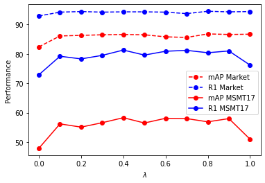
For $\lambda$ in Figure 5(a) we see stable performance for Market along different values after $\lambda=0.1$, while for MSMT17 we see a peak at $\lambda=0.4$, then a suitable decrease after this value. For both datasets, we see a performance drop for $\lambda=0.0$ (no $\mathcal{L}_{proxy}$), showing the proxy-based loss term has a positive impact on training while an equal contribution of both terms $\lambda=1.0$ hurts the performance mainly for MSMT17. Since MSMT17 is more challenging, we select $\lambda=0.4$ as the operational value. Further analysis of the impact of $\mathcal{L}_{proxy}$ is presented in Table 5.

The impact of $\tau$ is shown on Figure 5(b). The performance drops when $\tau$ is lower than $0.04$ for MSMT17 but a stable behavior for Market, while values greater than $0.06$ deteriorate the performance for both datasets. To achieve a good trade-off considering the dataset complexities, we choose $\tau=0.05$.

Impact of pooling operations in evaluation (PReID). As shown in Figure 2 in the main paper, the Evaluation is performed by a weighted combination of the decisions from Clean and Distortion-Adaptive backbones. The weights $W_{clean}$ and $W_{distortion}$ are the maximum magnitudes of the feature vectors for each query and gallery image pair for each backbone. Among the different pooling strategies, we choose Global Average Pooling (GAP), Global Max Pooling (GMP), and a combination of both (GAP+GMP) to check the impact on final performance. The performances are reported in Table 5, which is an extension of Table 6 from the main paper. Note that in this case, the pooling operations are just to calculate the magnitudes, since the final representation, as explained in section 5.2 of the main paper, is always obtained by the element-wise sum of the output of the GAP and GMP layers for PReID.

We see among GAP, GMP, and GAP+GMP, we have a similar performance in evaluation, with a slighter improvement for GAP. All of them have similar performances over the final result showing our proposed fusion strategy is robust to different pooling operations.

Code will be made publicly available upon acceptance. The LD datasets will be made available for academic use upon acceptance.

References

- (1) Jiankang Deng, Jia Guo, Evangelos Ververas, Irene Kotsia, and Stefanos Zafeiriou. Retinaface: Single-shot multi-level face localisation in the wild. In Proceedings of the IEEE/CVF conference on computer vision and pattern recognition, pages 5203–5212, 2020.
- (2) Yixiao Ge, Dapeng Chen, and Hongsheng Li. Mutual mean-teaching: Pseudo label refinery for unsupervised domain adaptation on person re-identification. arXiv preprint, arXiv:2001.01526, 2020.
- (3) Alexander Hermans, Lucas Beyer, and Bastian Leibe. In defense of the triplet loss for person re-identification. arXiv preprint, arXiv:1703.07737, 2017.
- (4) Nathan D Kalka, Brianna Maze, James A Duncan, Kevin O’Connor, Stephen Elliott, Kaleb Hebert, Julia Bryan, and Anil K Jain. Ijb–s: Iarpa janus surveillance video benchmark. In 2018 IEEE 9th international conference on biometrics theory, applications and systems (BTAS), pages 1–9. IEEE, 2018.
- (5) Minchul Kim, Anil K. Jain, and Xiaoming Liu. Adaface: Quality adaptive margin for face recognition. In Proceedings of the IEEE/CVF Conference on Computer Vision and Pattern Recognition (CVPR), pages 18750–18759, June 2022.
- (6) Diederik P Kingma and Jimmy Ba. Adam: A method for stochastic optimization. arXiv preprint arXiv:1412.6980, 2014.
- (7) Antti Tarvainen and Harri Valpola. Mean teachers are better role models: Weight-averaged consistency targets improve semi-supervised deep learning results. Advances in neural information processing systems, 30, 2017.
- (8) Yunpeng Zhai, Qixiang Ye, Shijian Lu, Mengxi Jia, Rongrong Ji, and Yonghong Tian. Multiple expert brainstorming for domain adaptive person re-identification. arXiv preprint, arXiv:2007.01546, 2020.
- (9) Kaipeng Zhang, Zhanpeng Zhang, Zhifeng Li, and Yu Qiao. Joint face detection and alignment using multitask cascaded convolutional networks. IEEE signal processing letters, 23(10):1499–1503, 2016.