CGA-PoseNet: Camera Pose Regression via
a 1D-Up Approach to Conformal Geometric Algebra
Thanks: Citation:
Authors. Title. Pages…. DOI:000000/11111.
Abstract
We introduce CGA-PoseNet, which uses the 1D-Up approach to Conformal Geometric Algebra (CGA) to represent rotations and translations with a single mathematical object, the motor, for camera pose regression. We do so starting from PoseNet, which successfully predicts camera poses from small datasets of RGB frames. State-of-the-art methods, however, require expensive tuning to balance the orientational and translational components of the camera pose.This is usually done through complex, ad-hoc loss function to be minimized, and in some cases also requires 3D points as well as images. Our approach has the advantage of unifying the camera position and orientation through the motor. Consequently, the network searches for a single object which lives in a well-behaved 4D space with a Euclidean signature. This means that we can address the case of image-only datasets and work efficiently with a simple loss function, namely the mean squared error (MSE) between the predicted and ground truth motors. We show that it is possible to achieve high accuracy camera pose regression with a significantly simpler problem formulation. This 1D-Up approach to CGA can be employed to overcome the dichotomy between translational and orientational components in camera pose regression in a compact and elegant way.
Keywords Camera Pose Regression Conformal Geometric Algebra Computer Vision

1 Introduction
By camera pose regression we refer to the prediction of the camera position and orientation which is fundamental for many computer vision applications [1], including augmented reality [2, 3], robotics [4, 5] and autonomous driving [6]. It has been historically solved via 2D-2D or 2D-3D feature matching methods, most famously the SIFT [7], SURF [8] or ORB [9] algorithms. Although very accurate, feature-based methods fail with texture-less objects, in cluttered scenes or in realistic weather conditions, and require a large database of features [10, 11, 12].
For this reason, several deep learning methods have been proposed in the literature. Despite not being as accurate as SIFT, deep neural networks can deal with smaller images and demonstrate high generalizability and faster inference times, even on small datasets [13, 14, 15, 16, 17]. No matter which architecture is employed, however, the orientational and translational components of the camera pose are generally still represented as two different mathematical objects which require separate treatments [18, 19, 20, 21, 22, 23, 24]. This makes the pose regression task more expensive as it adds further tuning of the loss function on top of the hyperparameter tuning for a successful pose estimation.
In this work, we reformulate the problem initially posed in [22] of learning the camera pose from RGB images by representing translation and rotation with a single mathematical object, the motor. Motors sit in a 4D space with Euclidean signature, i.e. with all basis vectors squaring to (see Figure 1). Our approach has three main advantages:
- •
A joint prediction of the camera position and orientation, unlike most previous literature which requires a tuneable weighting between the two. Note that we could have also used other elegant representations of rigid body transformations (screw theory/Plücker coordinates, CGA etc), but our 1D-Up approach to CGA provides a base space with Euclidean signature (therefore no inherent null structures) which lends itself to the construction of simple loss functions.
- •
The Euclidean signature of the space implies a simple, well-behaved loss function, namely the MSE between original and predicted motors. MSE is normally used in regression problems and easily computed. Loss functions presented in the literature, in fact, require an additional search over the weights for the orientational and translational components, which are dataset specific and add to the training complexity.
- •
Notation. We will employ boldface lowercase letters for vectors (e.g. ) and boldface uppercase letters for matrices (e.g. ) when dealing with 3D Euclidean geometry. For Geometric Algebra (GA), on the other hand, we will stick to the notation commonly employed in the field [26, 27], hence we will use simple lowercase letters for vectors (e.g. , …), uppercase letters for elements with grade 2 or higher (e.g. rotors , …) or elements in CGA (e.g. ) and Greek letters for scalars (e.g. ).
2 Related Work
Problem formulation. We wish to estimate camera pose , with via a deep neural network given an RGB image taken by a camera . This is usually posed as a supervised learning problem in which the network predicts given the label , with being the camera position and the camera orientation expressed as a quaternion [21, 22, 24].
Choosing the loss function. Much of the attention in camera pose regression problems has been focused on the loss function to be minimized rather than on the choice of representations for rotations and translations.
In [22], the rotational and the translational part are empirically weighted together as follows
| (1) |
in which is a weighting scalar. However, the choice of is non trivial and a grid search is required. The optimal value was found to be “the ratio between expected error of position and orientation at the end of training", which is not intuitive. Moreover, the value of varies significantly for each dataset, even if the volumes spanned by the datasets are comparable. For example, for the indoor datasets which are all , the optimal was found to be .
A similar range of values of is seen in Walch et al., who also used Equation 1 in [25]: the pretrained GoogLeNet is followed by LSTM modules with two different fully connected layers, one for the position and one for the orientation, as last layers.
The loss function of Equation 1 has also been employed in [19]. In it, a pretrained ResNet50 convolutional neural network is used to extract features for each image, which are then reshaped into graph form and input to a graph neural network (GNN) to predict position and orientation. This more complex architecture allowed Elmoogy et al. to be less strict on the choice of and empirically fix for indoor scenes and for outdoor scenes.
A similar weighting has been proposed in [24]. Xu et al. employed 2D trajectories of pedestrians to estimate the camera pose rather than RGB images only, and found that the weight parameter does not have a significant impact on the regression accuracy.
Weighting the translational and rotational parts is hence heavily dependent on the kind of datasets available and the chosen architecture.
The authors of [22] proposed a more advanced weighting strategy in [21]:
| (2) |
with being a learned weight and the variance modelled through homoscedastic uncertainty. This probabilistic deep learning approach is superior to the -weighting, but nonetheless still a weighting approach, with and to be learned and possibly differing from each other by several orders of magnitude.
Also in [21], a weighting-free approach is suggested: geometric reprojection error is used to combine the rotational and translational components into a single scalar loss. The geometric reprojection function is introduced, that maps a 3D point to 2D image coordinates :
| (3) |
where is defined via
| (4) |
with , the intrinsic camera calibration matrix and the rotation matrix corresponding to . The proposed loss takes the norm of the reprojection error between the predicted and ground truth camera pose:
| (5) |
In which is a subset of all the points in image . Despite the high accuracy of this approach, the amount of computation required at each learning iteration is significantly higher than that required by Equations 1-2. In addition, further discussion is needed to choose the most appropriate norm to be minimized.
The dichotomy between rotational and positional components is also present in works that adopt completely different regression strategies. This is the case in Chen et al., who suggested an ad-hoc parameterization in [18]: DirectionNet factorizes relative camera pose, specified by a 3D rotation and a translation direction, into a set of 3D direction vectors: the relative pose between two images, however, is still inferred in two steps for the rotation (DirectionNet-R) and the translation (DirectionNet-T) components.
Works like [18, 21] show that efforts in unifying the rotational and translational components correspond to better positional and rotational estimation. On the other hand, they are significantly less intuitive compared to the original PoseNet work [22]. In this work we wish to preserve the PoseNet pipeline, which is simple and successful, but also to avoid the rotational and translational weighting. We do so through a new mathematical representation for camera pose.
Rotation representations. While the position is most simply learned in Euclidean space, there are several possible ways to represent rotations. These include Euler angles, axis-angle form, rotation matrices, quaternions or, in GA, rotors and bivectors [28, 29, 30, 31].
It has been shown how different rotation representations might impact learning algorithms [32, 31, 33, 34]. Euler angles, for example, suffer from gimbal lock, rotation matrices are over-parametrised and their orthogonality can be difficult to enforce in learning algorithms, and quaternions have a double mapping for each rotation. Already in [32] the limitations of Euler angles and quaternions were highlighted when differentiation or integration operations were involved. Zhou et al., in [34] and Saxena et al. in [33] both suggested that the discontinuity in the mapping from the rotation matrix onto a given representation space is responsible for large regression errors. In [31], the discontinuity issue is bypassed by representing rotations exclusively via rotors and bivectors in GA.
While most of the camera pose regression problems employ quaternions to represent rotation, the potential of GA in learning problems is still largely uncharted.
3 Method
The main idea of our paper is to represent camera poses with motors in a specific space. In this Section, we will provide the reader with the fundamental notions to understand the motor representation. We will first present basic definitions of GA in Section 3.1: grades, the geometric product, the rotor and the reversion operator. We will then add two additional basis vectors to our space and map GA onto CGA in Section 3.2. In CGA, rigid body transformations are conveniently represented by rotors. Lastly, we will use as our origin to drop one dimension and work with a 1D-Up CGA space, which is a spherical space with curvature , in Section 3.3.
3.1 Geometric Algebra
Starting from the second half of the last century, GA has found application in many fields, including physics [26, 35], computer vision [36, 37, 38], graphics [39, 40] and molecular modelling [41, 42, 43].
GA is an algebra of geometric objects, which are built up via the geometric product. Given two GA vectors , the geometric product is defined as
| (6) |
in which represents the inner product and represents the outer product. The outer product allows to define an object , which we call an -blade with grade . Therefore, scalars are grade 0, vectors are grade 1, bivectors are grade 2, trivectors are grade 3, etc. A linear combination of -blades is called an -vector. A linear combination of different -vectors is a multivector. In Equation 6, the inner product gives a scalar proportional to the cosine of the angle between and the outer product yields a bivector, which corresponds to the (signed) area of the parallelogram with sides . Hence is a multivector, since it results from the sum of a scalar and a bivector, which have different grades: this is a substantial difference between geometric algebra and linear algebra.
Given a geometric product of vectors in an -D space where , we define the reversion operator . If we scale so that the expression
| (7) |
preserves both lengths and angles. This can be verified since and . Hence, it can be shown that represents a rotation in GA. If is even, then is called a rotor. “Sandwiching" a GA object between a rotor and its reverse, as shown in Equation 7, always results in a rotation of the object.
A rotor is equivalent to a quaternion in 3D, it has fewer parameters than a rotation matrix, it does not suffer from gimbal lock and can be extended to any arbitrary dimension. We will show how translations can also be represented via rotors in Section 3. We refer the reader to [26] for a more complete discussion of GA fundamentals.
3.2 Conformal Geometric Algebra (CGA)
A geometric algebra with basis vectors that square to and basis vectors that square to is indicated via . CGA extends a geometric algebra by two additional basis vectors and , mapping onto [38]. Hence, CGA maps the 3D geometric algebra , spanned by the basis vectors , to , spanned by the basis vectors .
The two additional basis vectors allow us to define two quantities:
| (8) |
i.e. the infinity vector, and
| (9) |
i.e. the origin vector. Points in a geometric algebra are mapped to null vectors in through and according to the equation
| (10) |
In CGA, reflections, rotations, translations and other geometric operations can all be conveniently represented as rotors. These rotors act on objects by sandwiching as in Equation 7. In addition, CGA offers an intuitive representation of geometrical objects such point pairs, lines, planes, circles and spheres.
3.3 1D-Up CGA
When dealing with transformations in Euclidean geometry in CGA, the point at infinity is kept constant. However, we can work with non-Euclidean geometries if we keep different quantities constant. For example by keeping constant, it can be shown that we are left with a hyperbolic geometry. Similarly, when is kept constant we are left with a spherical geometry. Note how, by keeping either one of the bases or constant, we have only additional basis vector compared to 3D GA (hence the name “1D-Up") instead of two as in CGA (which is a “2D-Up" space compared to 3D GA). [44, 45, 27].
In this paper we work with the latter case, in which is kept constant and is our origin. The main advantages of the 1D-Up approach are: (1) a lower dimensionality of the space compared to CGA, (2) that the Euclidean nature of the space (i.e. that all basis vectors square to ) allows us to construct a simple loss function that is invariant under rigid body transformations and (3) that both translations and rotations can be expressed as rotors, just as in the 2D Up space.
We now explain how to represent translations and rotations in a 1D-Up CGA. A translation by a 3D Euclidean vector has an equivalent rotor in 4D spherical geometry given by:
| (11) |
where is a factor related to the radius of curvature of the spherical space. Note that translation by a vector is now performed via a , composed of a scalar part (with grade 0) and a bivector part (with grade 2). To translate an object in 1D-Up CGA we will “sandwich" it between and , as explained in Section 2.2.
It can be shown that a rotor in 3D Euclidean geometry is still in 4D spherical geometry. To rotate an object in 1D-Up CGA we will again “sandwich" it between and . The rigid body motion (i.e. translation and rotation) of an object into in the 1D-Up CGA can hence be expressed as:
| (12) |
in which is the corresponding representation in of a point in , given by
| (13) |
and in which we call the object a motor. The motor is obtained from the geometric product of , the translation rotor, with , the rotation rotor. is a multivector with a scalar part (grade 0), a bivector part (grade 2), and a quadrivector part (grade 4). It can hence be written as
| (14) |
with , and . A 1D-Up CGA motor hence has a total of 8 coefficients . Note that the motor is constrained to satisfy .
We can then represent the camera pose, i.e. its orientation (a rotation) its position (a translation), with the 8 components of a single motor. Because we are working in this spherical space with a Euclidean signature, it will be possible to construct loss functions on motors in this space which are well-behaved under minimisation.
4 Experiments
A motor has a total of 8 coefficients to be predicted, one scalar, one quadrivector and 6 bivectors. This means 1 more parameter with respect to , which are 3 + 4 = 7, but a single search space for our network to span.
We employed the Cambridge Landmarks [22] and the Scenes [46] datasets for our experiments. We recast the original labels from for the Landmarks datasets (or from , for the Scenes dataset) into the motor coefficients . We work in a spherical space with curvature , where the rotation is the same as the rotation in Euclidean space and the translation uses the vector . This can be done easily as the rotor is isomorphic to the quaternion in 3D, while the corresponding can be found from Equation 11. The pose motor is obtained as .
Hence, CGA-PoseNet extends PoseNet to regress the camera’s pose expressed as a motor relative to a scene starting from a RGB image. The original architecture Inception v3, derived from [47, 48], is pretrained on ImageNet. We then:
- •
Substitute the training labels ([ or ) with motors ;
- •
Substitute the final softmax layer with a fully connected layer with dimensionality 8, to match the number of coefficients of the motor;
- •
Use the MSE loss between predicted and ground truth motors during training.
| Dataset | Train | Test | Area / Volume | |
|---|---|---|---|---|
| Street | 1500 | 1500 | 50000 | 1000 |
| Great Court | 1000 | 1000 | 8000 | 200 |
| King’s | 1220 | 343 | 5600 | 200 |
| St. Mary’s | 1487 | 530 | 4800 | 200 |
| Old Hospital | 895 | 182 | 2000 | 200 |
| Shop | 231 | 103 | 875 | 10 |
| RedKitchen | 3000 | 1000 | 10 | |
| Office | 2000 | 2000 | 10 | |
| 7 Scenes | 1000 | 1000 | 10 | |
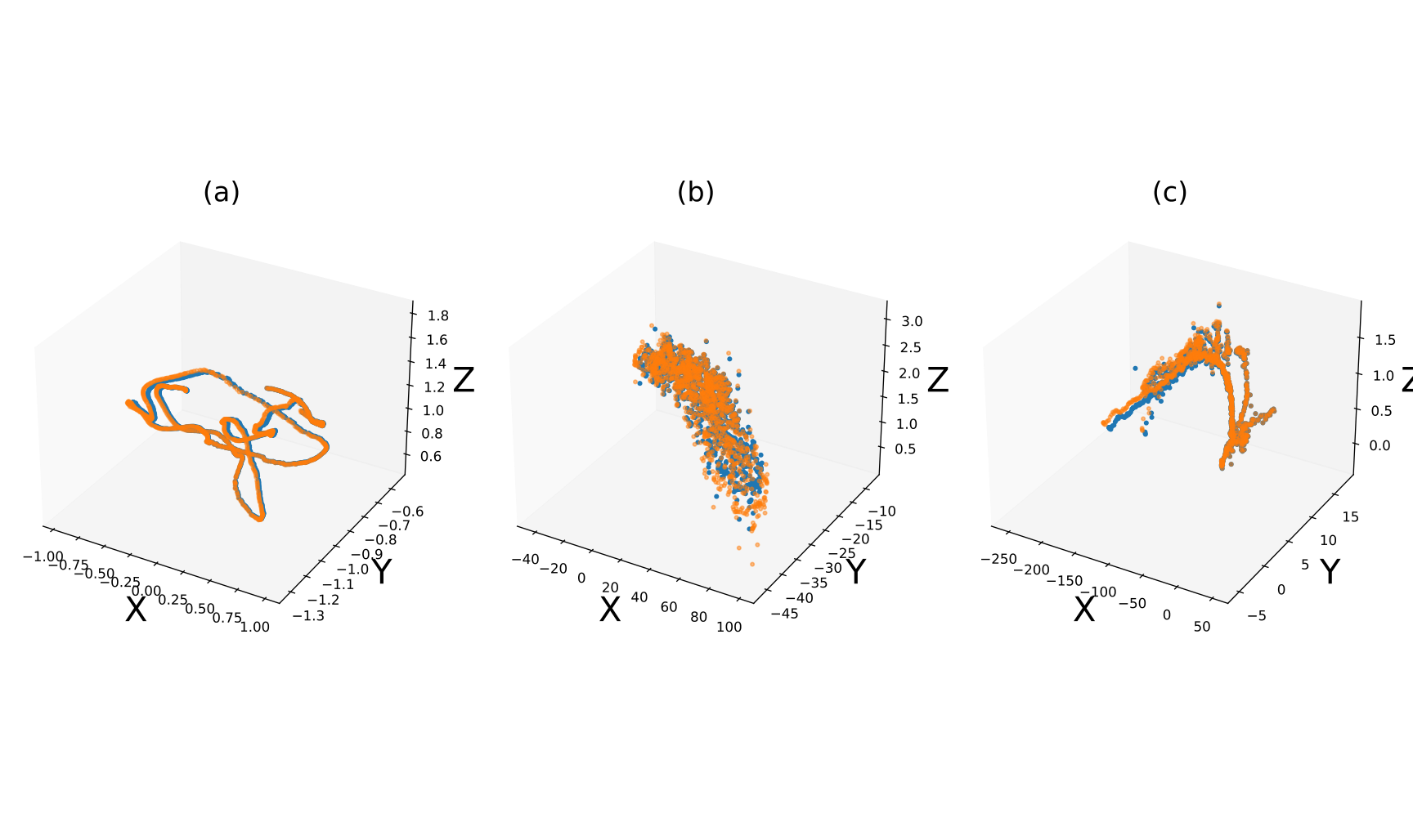
Discussing , the curvature of the space. is the only free parameter in our approach and it controls the curvature of the 4D spherical space. In contrast to the weighing parameter of [19, 22, 24], there is no need for a grid search, as we will see that it can simply be chosen to be directly proportional to the dataset area, before any training begins. Equivalently, by normalizing the input position data, it is possible to keep fixed to a desired value.
As the spherical space tends to the flat Euclidean space [27]. For , however, the motor coefficients containing are several orders of magnitude smaller than the others, negatively impacting the training. On the other hand, a small makes the curvature of the spherical space noticeable, meaning that our motor is not suitable to represent a roto-translation of a camera in the real world.
To choose an appropriate , we plotted the positional component associated with each frame (i.e. the camera trace) for every dataset. We compared the trace in Euclidean space (i.e. ) with the trace in spherical space as a function of . Examples are given in Figure 2. The processing of extracting the trace in spherical space is explained in Section 4.3.
As we wish to represent a camera pose in 3D Euclidean space, we empirically chose in such a way that (1) the curvature is not noticeable, i.e. and (2) the motor coefficients are all within the same order of magnitude. For this reason, can be picked to be proportional to the area spanned by the dataset. The choices of for each of the datasets are summarized in Table 1.
4.1 Datasets
Cambridge Landmarks [22] includes 6 datasets of outdoor scenes, namely Street, Great Court, King’s College, St. Mary’s Church, Old Hospital and Shop Facade, spanning areas ranging from up to . Each dataset includes a sequence of RGB frames with their corresponding labels, i.e. the motor coefficients representing the camera pose. Labels are generated via structure from motion, as described in [49]. We employed no more than 1500 frames for training. This is to show how, even with a smaller training set size, comparable results to the SoTA can be achieved. Each dataset presents significant clutter and the training and testing trajectories are non overlapping.
7 Scenes [46] includes 7 datasets of indoor scenes, namely Office, Pumpkin, Red Kitchen, Heads, Fire, Stairs and Chess, each spanning a volume not larger than . The dataset was intended for RGB-D relocalization and has been captured through a Kinect RGB-D sensor. We employed no more than 3000 frames for training.
4.2 Training details
We train PoseNet in a supervised fashion by labeling each frame with the corresponding camera pose . The loss we minimize is
| (15) |
where and are the predicted and ground truth motors, respectively. The network has been trained three times for each dataset with batch size , for epochs and implementing early stopping with patience during the last run to avoid overfitting. Results are measured with the weights obtained after the third training session. The optimizer has been kept to Adam with exponentially decaying learning rate, with initial value and decay rate of . The hyperparameters have been chosen empirically according to the chosen datasets, and combinations of , , , have also been tested but found to be suboptimal. The training takes an average of ms per learning step, corresponding to about s per epoch assuming the training set contains 1000 images.
We leveraged transfer learning as discussed in [22] and employed the weights from (see [50]) for prior training of CGA-PoseNet to ensure a successful regression even on small datasets such as those employed in this paper.
All the experiments have been written as Jupyter notebooks on Google Colaboratory and run on a NVIDIA Tesla T4 GPU at 1.59 GHz. The Machine Learning architectures have been implemented via the Keras API of Tensorflow, 3D rotations have been handled through the Spatial Transformations package of Scipy and Geometric Algebra operations have been performed via the Clifford library [51]. The Jupyter notebooks, predictions and measurements files are all included as Supplementary Materials.
4.3 Metrics
In order to evaluate the goodness of this regression strategy, we evaluate two metrics: (i) positional error and (ii) rotational error.
The positional and rotational error are computed by extracting the translational and rotational components from and . Given a motor , this is done as follows:
- •
evaluate the displacement vector by transforming the origin, , with (the origin is not affected by rotation so only the translation will have any effect), i.e. . The displacement vector has the form
- •
project onto via Eq. 13 (i.e. ). From and we compute the positional error
- •
evaluate the translation in spherical geometry
- •
retrieve the rotor as . From and we compute the rotational error
We will define positional error between original position and predicted position as:
| (16) |
as this was found to perform the best with the chosen datasets and it does not increase quadratically with magnitude. In addition, it is in agreement with the norm chosen in the loss functions of [21] and Chapter 3 of [52].
The rotational error between original rotation and predicted rotation has been inspired by the error to assess regressions on rotations in [31, 34] and is defined as:
| (17) |
where indicates the scalar part of the argument. Ideally, if , then . Hence, the rotational error is bounded in , which is what we would expect in rotation regression problems.
5 Results
| Scene | PoseNet [22] | Bayesian PoseNet [20] | PoseNet LSTM [25] | PoseNet Weights [21] | PoseNet Geom. Repr. [21] | CGA- PoseNet | |
| Great Court | - | - | - | 7.00m, 3.65∘ | 6.83m, 3.47∘ | 3.77m, 4.27∘ | 78.3 |
| King’s | 1.92m, 5.40∘ | 1.74m, 4.06∘ | 0.99m, 3.65∘ | 0.99m, 1.06∘ | 0.88m, 1.04∘ | 1.36m, 1.85∘ | 95.6 |
| Old Hospital | 2.31m, 5.38∘ | 2.57m, 5.14∘ | 1.51m, 4.29∘ | 2.17m, 2.94∘ | 3.20m, 3.29∘ | 2.52m, 2.90∘ | 99.4 |
| St. Mary’s | 2.65m, 8.48∘ | 2.11m, 8.38∘ | 1.52m, 6.68∘ | 1.49m, 3.43∘ | 1.57m, 3.32∘ | 2.12m, 2.97∘ | 87.5 |
| Shop | 1.46m, 8.08∘ | 1.25m, 7.54∘ | 1.18m, 7.44∘ | 1.05m, 3.97∘ | 0.88m, 3.78∘ | 0.74m, 5.84∘ | 89.3 |
| Street | - | - | - | 20.7m, 25.7∘ | 20.3m, 25.5∘ | 19.6m,19.9∘ | 9.25 |
| Chess | 0.32m, 6.60∘ | 0.37m, 7.24∘ | 0.24m, 5.77∘ | 0.24m, 5.77∘ | 0.13m, 4.48∘ | 0.26m, 6.34∘ | - |
| Pumpkin | 0.49m, 8.12∘ | 0.61m, 7.08∘ | 0.33m, 7.00∘ | 0.25m, 4.82∘ | 0.26m, 4.75∘ | 0.22m, 5.18∘ | - |
| Fire | 0.47m, 14.0∘ | 0.43m, 13.7∘ | 0.34m, 11.9∘ | 0.27m, 11.8∘ | 0.27m, 11.3∘ | 0.28m, 10.3∘ | - |
| Heads | 0.30m, 12.2∘ | 0.31m, 12.0∘ | 0.21m, 13.7∘ | 0.18m, 12.1∘ | 0.17m, 13.0∘ | 0.17m, 7.98∘ | - |
| Office | 0.48m, 7.24∘ | 0.48m, 8.04∘ | 0.30m, 8.08∘ | 0.20m, 5.77∘ | 0.19m, 5.55∘ | 0.26m, 7.23∘ | - |
| Red Kitchen | 0.58m, 8.34∘ | 0.58m, 7.54∘ | 0.37m, 8.83∘ | 0.24m, 5.52∘ | 0.23m, 5.35∘ | 0.55m, 16.7∘ | - |
| Stairs | 0.48m, 13.1∘ | 0.48m, 13.1∘ | 0.40m, 13.7∘ | 0.37m, 10.6∘ | 0.35m, 12.4∘ | 0.17m, 12.0∘ | - |


Results are summarized in Table 2. We benchmarked our results with 5 different variations of the original PoseNet. Note how our CGA-PoseNet yields superior results in [22] and superior to comparable results in [20, 21, 25], even for larger and more difficult datasets like Street and Great Court. Specifically, our CGA-PoseNet approach is superior in every dataset analyzed to the results in [22], and superior in 6 out of 13 datasets to [21] (with loss ) and in 7 out of 13 datasets (with loss ) despite having the simplest problem formulation of all of the compared approaches: our MSE loss, shown in Equation 15, is significantly less computationally expensive than losses of Equations 1, 2 and 5, but still allowed us to regress the camera pose accurately.
It is worth noting that our approach does not employ any additional information to the camera pose labels. For example, we completely discard the 3D points of the datasets on which the geometric reprojection error of [21] is based. The Cambridge Landmarks dataset, for example, includes 3D points, which are employed to formulate the loss . Our approach yields comparable result to it without including any geometrical information of the scene during training, which makes CGA-PoseNet particularly suitable in scenarios in which points annotations are not available in the training set.
Also note how our motor representation of the camera pose yields superior results to the approach in [20], which includes the model uncertainty along with the 6 degrees-of-freedom representation of the camera pose, and generally superior results to the approach in [48], which includes an additional LSTM network at the output of PoseNet.
Aerial views of the predicted and ground truth camera poses for the Cambridge Landmarks are plotted in Figure 3, as in [22]. The resulting traces represent the positions of the camera in 3D Euclidean space associated to the frames of the test set and corresponding predictions. If we consider only projections, the positional errors can be even lower than those in Table 2. The orientation has also been plotted as a 3D scatter plot of the vector coefficients of (i.e. ) in Figure 4. As the positional and rotational errors are evaluated starting from the same quantity , they are highly correlated (see Figure 7). The positional and rotational error distribution over the test sets of selected datasets are shown in Figs. 5 and 6, respectively.
Lastly, we cross-checked the goodness of the pose predictions through point clouds. We generated the corresponding point clouds for four of the Cambridge Landmarks set with smaller sizes, namely King’s, St Mary’s, Old Hospital and Shop Facade, from frames through structure from motion [53]. We then measured the MSE between the point cloud with pose and the point cloud with pose over the test sets of the four landmarks. The point clouds are plotted in Figure 8: the point clouds in Euclidean space have been first projected onto the spherical space (via Eq. 13), then rotated and translated by and (via Eq. 12) and then projected back down to Euclidean space (via inverse Eq. 13), in which the MSE has been measured.

This test tells us two things: first, that rotating and translating a point cloud in a spherical space with a suitable is possible without noticeable deformation occurring, meaning that a motor in spherical space can be used to to give a good estimate of a camera pose in 3D Euclidean space; second, that the results obtained with point clouds are consistent with the positional errors of Table 2.
6 Conclusions
We have presented CGA-PoseNet, a GA approach for representing rotations and translations in the camera localization problem. To do this we used the 1D-Up approach to CGA, which unifies rotations and translations in a single object, the motor, which can be described by 8 (constrained) coefficients. We are also able to construct a well-behaved and simple cost function, thus eliminating the need for data dependent parameters.
We have used CGA-PoseNet to learn the camera poses, expressed as motors, of 13 datasets , and demonstrated that this approach allows a much simpler formulation of the loss function while giving results comparable, when not superior, to more complex approaches existing in the literature. Results obtained with CGA-PoseNet, moreover, are comparable to those obtained minimizing the geometric reprojection error, which requires the 3D points in the model in order to be trained, which means we can achieve similar results with much less information as input to our model.
This paper aims to present a proof of concept for a unifying approach to dealing with rotations and translations in camera pose problems. There is room for improvement in the results presented here – a more rigourous tuning of the training hyperparameters could potentially provide results surpassing state-of-the-art methods.

References
- [1] Sabera Hoque, Md Yasir Arafat, Shuxiang Xu, Ananda Maiti, and Yuchen Wei. A comprehensive review on 3d object detection and 6d pose estimation with deep learning. IEEE Access, 2021.
- [2] Fakhr-eddine Ababsa and Malik Mallem. Robust camera pose estimation using 2d fiducials tracking for real-time augmented reality systems. In Proceedings of the 2004 ACM SIGGRAPH international conference on Virtual Reality continuum and its applications in industry, pages 431–435, 2004.
- [3] Chandan K Sahu, Crystal Young, and Rahul Rai. Artificial intelligence (ai) in augmented reality (ar)-assisted manufacturing applications: a review. International Journal of Production Research, 59(16):4903–4959, 2021.
- [4] Timothy E Lee, Jonathan Tremblay, Thang To, Jia Cheng, Terry Mosier, Oliver Kroemer, Dieter Fox, and Stan Birchfield. Camera-to-robot pose estimation from a single image. In 2020 IEEE International Conference on Robotics and Automation (ICRA), pages 9426–9432. IEEE, 2020.
- [5] Lin Yen-Chen, Pete Florence, Jonathan T Barron, Alberto Rodriguez, Phillip Isola, and Tsung-Yi Lin. inerf: Inverting neural radiance fields for pose estimation. In 2021 IEEE/RSJ International Conference on Intelligent Robots and Systems (IROS), pages 1323–1330. IEEE, 2021.
- [6] Florian Sauerbeck, Lucas Baierlein, Johannes Betz, and Markus Lienkamp. A combined lidar-camera localization for autonomous race cars. SAE International Journal of Connected and Automated Vehicles, 5(12-05-01-0006):61–71, 2022.
- [7] David G Lowe. Distinctive image features from scale-invariant keypoints. International journal of computer vision, 60(2):91–110, 2004.
- [8] Herbert Bay, Andreas Ess, Tinne Tuytelaars, and Luc Van Gool. Speeded-up robust features (surf). Computer vision and image understanding, 110(3):346–359, 2008.
- [9] Ethan Rublee, Vincent Rabaud, Kurt Konolige, and Gary Bradski. Orb: An efficient alternative to sift or surf. In 2011 International conference on computer vision, pages 2564–2571. Ieee, 2011.
- [10] Alessandro Bergamo, Sudipta N Sinha, and Lorenzo Torresani. Leveraging structure from motion to learn discriminative codebooks for scalable landmark classification. In Proceedings of the IEEE Conference on Computer Vision and Pattern Recognition, pages 763–770, 2013.
- [11] Junqiu Wang, Hongbin Zha, and Roberto Cipolla. Coarse-to-fine vision-based localization by indexing scale-invariant features. IEEE Transactions on Systems, Man, and Cybernetics, Part B (Cybernetics), 36(2):413–422, 2006.
- [12] Bernhard Zeisl, Torsten Sattler, and Marc Pollefeys. Camera pose voting for large-scale image-based localization. In Proceedings of the IEEE International Conference on Computer Vision, pages 2704–2712, 2015.
- [13] Sovann En, Alexis Lechervy, and Frédéric Jurie. Rpnet: An end-to-end network for relative camera pose estimation. In Proceedings of the European Conference on Computer Vision (ECCV) Workshops, pages 0–0, 2018.
- [14] Iaroslav Melekhov, Juha Ylioinas, Juho Kannala, and Esa Rahtu. Relative camera pose estimation using convolutional neural networks. In International Conference on Advanced Concepts for Intelligent Vision Systems, pages 675–687. Springer, 2017.
- [15] Yoshikatsu Nakajima and Hideo Saito. Robust camera pose estimation by viewpoint classification using deep learning. Computational Visual Media, 3(2):189–198, 2017.
- [16] Jason R Rambach, Aditya Tewari, Alain Pagani, and Didier Stricker. Learning to fuse: A deep learning approach to visual-inertial camera pose estimation. In 2016 IEEE International Symposium on Mixed and Augmented Reality (ISMAR), pages 71–76. IEEE, 2016.
- [17] Kwang Moo Yi, Eduard Trulls, Yuki Ono, Vincent Lepetit, Mathieu Salzmann, and Pascal Fua. Learning to find good correspondences. In Proceedings of the IEEE conference on computer vision and pattern recognition, pages 2666–2674, 2018.
- [18] Kefan Chen, Noah Snavely, and Ameesh Makadia. Wide-baseline relative camera pose estimation with directional learning. In Proceedings of the IEEE/CVF Conference on Computer Vision and Pattern Recognition, pages 3258–3268, 2021.
- [19] Ahmed Elmoogy, Xiaodai Dong, Tao Lu, Robert Westendorp, and Kishore Reddy. Pose-gnn: Camera pose estimation system using graph neural networks. arXiv preprint arXiv:2103.09435, 2021.
- [20] Alex Kendall and Roberto Cipolla. Modelling uncertainty in deep learning for camera relocalization. In 2016 IEEE international conference on Robotics and Automation (ICRA), pages 4762–4769. IEEE, 2016.
- [21] Alex Kendall and Roberto Cipolla. Geometric loss functions for camera pose regression with deep learning. In Proceedings of the IEEE conference on computer vision and pattern recognition, pages 5974–5983, 2017.
- [22] Alex Kendall, Matthew Grimes, and Roberto Cipolla. Posenet: A convolutional network for real-time 6-dof camera relocalization. In Proceedings of the IEEE international conference on computer vision, pages 2938–2946, 2015.
- [23] Yu Xiang, Tanner Schmidt, Venkatraman Narayanan, and Dieter Fox. Posecnn: A convolutional neural network for 6d object pose estimation in cluttered scenes. arXiv preprint arXiv:1711.00199, 2017.
- [24] Yan Xu, Vivek Roy, and Kris Kitani. Estimating 3d camera pose from 2d pedestrian trajectories. In 2020 IEEE Winter Conference on Applications of Computer Vision (WACV), pages 2568–2577. IEEE, 2020.
- [25] Florian Walch, Caner Hazirbas, Laura Leal-Taixe, Torsten Sattler, Sebastian Hilsenbeck, and Daniel Cremers. Image-based localization using lstms for structured feature correlation. In Proceedings of the IEEE International Conference on Computer Vision, pages 627–637, 2017.
- [26] Chris Doran and Anthony Lasenby. Geometric algebra for physicists. Cambridge University Press, 2003.
- [27] Anthony N Lasenby. A 1d up approach to conformal geometric algebra: applications in line fitting and quantum mechanics. Advances in Applied Clifford Algebras, 30(2):1–16, 2020.
- [28] Qiang Fang, Kuang Zhao, Dengqing Tang, Zhengyuan Zhou, Yong Zhou, Tianjiang Hu, and Han Zhou. Euler angles based loss function for camera localization with deep learning. 2018 IEEE 8th Annual International Conference on CYBER Technology in Automation, Control, and Intelligent Systems (CYBER), pages 61–66. IEEE, 2018.
- [29] Zhiwu Huang, Chengde Wan, Thomas Probst, and Luc Van Gool. Deep learning on lie groups for skeleton-based action recognition. Proceedings of the IEEE conference on computer vision and pattern recognition, pages 6099–6108, 2017.
- [30] Dario Pavllo, David Grangier, and Michael Auli. Quaternet: A quaternion-based recurrent model for human motion. arXiv preprint arXiv:1805.06485, 2018.
- [31] Alberto Pepe, Joan Lasenby, and Pablo Chacón. Learning rotations. Conference on Applied Geometric Algebras in Computer Science and Engineering (AGACSE), 2021.
- [32] F Sebastian Grassia. Practical parameterization of rotations using the exponential map. Journal of graphics tools, 3(3):29–48, 1998.
- [33] Ashutosh Saxena, Justin Driemeyer, and Andrew Y Ng. Learning 3-d object orientation from images. 2009 ieee international conference on robotics and automation, pages 794–800. IEEE, 2009.
- [34] Yi Zhou, Connelly Barnes, Jingwan Lu, Jimei Yang, and Hao Li. On the continuity of rotation representations in neural networks. Proceedings of the IEEE/CVF Conference on Computer Vision and Pattern Recognition, pages 5745–5753, 2019.
- [35] David Hestenes. Space-time algebra. Springer, 2015.
- [36] Eduardo Bayro-Corrochano. Geometric algebra applications vol. I: Computer vision, graphics and neurocomputing. Springer, 2018.
- [37] Jaroslav Hrdina and Aleš Návrat. Binocular computer vision based on conformal geometric algebra. Advances in Applied Clifford Algebras, 27(3):1945–1959, 2017.
- [38] Rich Wareham, Jonathan Cameron, and Joan Lasenby. Applications of conformal geometric algebra in computer vision and graphics. In Computer algebra and geometric algebra with applications, pages 329–349. Springer, 2004.
- [39] Dietmar Hildenbrand. Geometric computing in computer graphics using conformal geometric algebra. Computers & Graphics, 29(5):795–803, 2005.
- [40] Dietmar Hildenbrand, Christian Perwass, Leo Dorst, and Daniel Fontijne. Geometric algebra and its application to computer graphics. In Eurographics (Tutorials), 2004.
- [41] Pieter Chys. Application of geometric algebra for the description of polymer conformations. The Journal of chemical physics, 128(10):104107, 2008.
- [42] Leo Dorst. Boolean combination of circular arcs using orthogonal spheres. Advances in Applied Clifford Algebras, 29(3):1–21, 2019.
- [43] Carlile Lavor and Rafael Alves. Oriented conformal geometric algebra and the molecular distance geometry problem. Advances in Applied Clifford Algebras, 29(1):1–15, 2019.
- [44] Anthony Lasenby. Recent applications of conformal geometric algebra. In Computer Algebra and Geometric Algebra with Applications, pages 298–328. Springer, 2004.
- [45] Anthony Lasenby. Rigid body dynamics in a constant curvature space and the ‘1d-up’approach to conformal geometric algebra. In Guide to geometric algebra in practice, pages 371–389. Springer, 2011.
- [46] Jamie Shotton, Ben Glocker, Christopher Zach, Shahram Izadi, Antonio Criminisi, and Andrew Fitzgibbon. Scene coordinate regression forests for camera relocalization in rgb-d images. In Proceedings of the IEEE conference on computer vision and pattern recognition, pages 2930–2937, 2013.
- [47] Christian Szegedy, Wei Liu, Yangqing Jia, Pierre Sermanet, Scott Reed, Dragomir Anguelov, Dumitru Erhan, Vincent Vanhoucke, and Andrew Rabinovich. Going deeper with convolutions. In Proceedings of the IEEE conference on computer vision and pattern recognition, pages 1–9, 2015.
- [48] Christian Szegedy, Vincent Vanhoucke, Sergey Ioffe, Jon Shlens, and Zbigniew Wojna. Rethinking the inception architecture for computer vision. In Proceedings of the IEEE conference on computer vision and pattern recognition, pages 2818–2826, 2016.
- [49] Changchang Wu. Towards linear-time incremental structure from motion. In 2013 International Conference on 3D Vision-3DV 2013, pages 127–134. IEEE, 2013.
- [50] Jia Deng, Wei Dong, Richard Socher, Li-Jia Li, Kai Li, and Li Fei-Fei. Imagenet: A large-scale hierarchical image database. In 2009 IEEE conference on computer vision and pattern recognition, pages 248–255. Ieee, 2009.
- [51] Hugo Hadfield, Eric Wieser, Alex Arsenovic, Robert Kern, and The Pygae Team. pygae/clifford.
- [52] Alex Guy Kendall. Geometry and uncertainty in deep learning for computer vision. PhD thesis, University of Cambridge, UK, 2019.
- [53] LLC Agisoft. Agisoft metashape user manual: professional edition, version 1.5. Accessed: Jan, 16:2019, 2019.