1Introduction

UFIFT-QG-23-02

Coincident Massless, Minimally Coupled Scalar Correlators on General Cosmological Backgrounds

E. Kasdagli^∗, M. Ulloa^† and R. P. Woodard^‡

Department of Physics, University of Florida,
Gainesville, FL 32611, UNITED STATES

ABSTRACT

The coincidence limits of the massless, minimally coupled scalar propagator and its first two derivatives have great relevance for the project of summing up the leading logarithms induced by loops of inflationary gravitons. We use dimensional regularization to derive good analytic approximations for the three quantities on a general cosmological background geometry which underwent inflation.

PACS numbers: 04.50.Kd, 95.35.+d, 98.62.-g

^∗ e-mail: kasdaglie@ufl.edu

^† e-mail: m.ulloacalzonzin@ufl.edu

^‡ e-mail: woodard@phys.ufl.edu

1 Introduction

We are interested in quantum field theory on a homogeneous, isotropic and spatially flat geometry with scale factor $a(t)$ , Hubble parameter $H(t)$ , and first slow roll parameter $\epsilon(t)$ ,

ds^{2}=-dt^{2}+a^{2}(t)d\vec{x}\!\cdot\!d\vec{x}\qquad,\qquad H(t)\equiv\frac{\dot{a}}{a}\quad,\quad\epsilon(t)\equiv-\frac{\dot{H}}{H^{2}}\;.

(1)

The dynamical system we study is the massless, minimally coupled scalar,

\mathcal{L}=-\frac{1}{2}\partial_{\mu}\Phi\partial_{\nu}\Phi g^{\mu\nu}\sqrt{-g}\;.

(2)

This system is of great interest because it includes the free inflaton, as well as dynamical gravitons [1]. What we specifically seek are coincidence limits of the scalar propagator $i\Delta(x;x^{\prime})$ and its first two derivatives,

A(t)\equiv i\Delta(x;x^{\prime})\Bigl|_{x^{\prime}=x},B_{\mu}(t)\equiv\partial_{\mu}i\Delta(x;x^{\prime})\Bigl|_{x^{\prime}=x},C_{\mu\nu}(t)\equiv\partial_{\mu}\partial_{\nu}^{\prime}i\Delta(x;x^{\prime})\Bigl|_{x^{\prime}=x}.

(3)

These correlators are crucial in deriving the curvature-dependent effective potentials [2] needed to apply Starobinsky’s stochastic formalism [3, 4] to the task of re-summing the large temporal and spatial logarithms induced by loops of inflationary gravitons [5, 6, 7, 8, 9, 10, 11].

To better motivate this study, note first that graviton loop corrections on de Sitter background typically involve logarithms of the scale factor $a$ . For example, the Coulomb potential of a stationary charge $Q$ becomes [6],

\Phi(t,r)=\frac{Q}{4\pi ar}\Biggl\{1+\frac{2G}{3\pi a^{2}r^{2}}+\frac{2GH^{2}}{\pi}\ln(aHr)+O(G^{2})\Biggr\}\;,

(4)

where $G$ is Newton’s constant. Similarly, a single graviton loop enhances the electric field strength of a plane wave photon to [7],

F^{0i}(t,\vec{x})=F^{0i}_{0}(t,\vec{x})\Biggl\{1+\frac{2GH^{2}}{\pi}\ln(a)+O(G^{2})\Biggr\}\;,

(5)

where $F^{0i}_{0}(t,\vec{x})$ is the tree order field strength. The analogous results for the mode function $u(t,k)$ of a plane wave graviton [9] and the Newtonian potential of a stationary mass $M$ [11] are,

	$\displaystyle u(t,k)$	$\displaystyle\!\!\!=\!\!\!$	$\displaystyle u_{0}(t,k)\Biggl\{1+\frac{16\pi GH^{2}}{3\pi}\ln^{2}(a)+O(G^{2})\Biggr\}\;,\qquad$		(6)
	$\displaystyle\Psi(t,r)$	$\displaystyle\!\!\!=\!\!\!$	$\displaystyle-\frac{GM}{ar}\Biggl\{1+\frac{103G}{15\pi a^{2}r^{2}}-\frac{8GH^{2}}{\pi}\ln^{3}(a)+O(G^{2})\Biggr\}.\qquad$		(7)

Even though the loop-counting parameter $GH^{2}\mathrel{\raise 1.29167pt\hbox{$<$\kern-7.5pt\lower 4.30554pt\hbox{$\sim$}}}10^{-10}$ is very small, the steady growth of $\ln[a(t)]$ must eventually cause perturbation theory to break down if inflation persists for a large number of e-foldings. Understanding what happens after that point requires some sort of nonperturbative resummation technique. And exploring the fascinating question of what effects might persist to the current epoch requires a technique that is not specialized to de Sitter but can be applied to any geometry (1) which has experienced a phase of primordial inflation.

Starobinsky’s stochastic formalism [3, 4] can be proven to capture the leading logarithms of scalar potential models to all orders [12], but the derivative interactions of quantum gravity invalidate the proof, and direct calculation reveals that the technique fails even at one loop [13]. Nonlinear sigma models such as,

\mathcal{L}=-\frac{1}{2}\Bigl(1+\frac{1}{2}\lambda\Phi\Bigr)^{2}\partial_{\mu}\Phi\partial_{\nu}\Phi\;,

(8)

possess similar derivative interactions, and induce the same sorts of large logarithms on de Sitter, but without the complicating features of tensor indices and gauge fixing. Much work has been done on such models in order to better understand quantum gravity [12, 14, 15, 16, 2, 17]. It has recently been shown that the large logarithms of nonlinear sigma models can be resummed by combining a variant of Starobinksy’s technique with a variant of the renormalization group [2]. Applying the renormalization group does not concern us here but facilitating Starobinsky’s formalism motivates the current study.

One applies Starobinsky’s technique to (8) by first writing the exact field equation,

\frac{\delta S[\Phi]}{\delta\Phi}=\Bigl(1+\frac{1}{2}\lambda\Phi\Bigr)\partial_{\mu}\Bigl[\Bigl(1+\frac{1}{2}\lambda\Phi\Bigr)\sqrt{-g}\,g^{\mu\nu}\partial_{\nu}\Phi\Bigr]=0\;.

(9)

Now note that a constant scalar background represents a field strength renormalization of the free propagator,

\Phi(x)=\Phi_{0}\qquad\Longrightarrow\qquad\Bigl\langle\Omega\Bigl|\Phi(x)\Phi(x^{\prime})\Bigr|\Omega\Bigr\rangle=\frac{i\Delta(x;x^{\prime})}{(1+\frac{1}{2}\lambda\Phi_{0})^{2}}\;.

(10)

We can define an effective force due to undifferentiated scalars by integrating out the differentiated fields from the interaction part of (9) using (10),

-V^{\prime}_{\rm eff}(\Phi_{0})\sqrt{-g}=\Bigl(1+\frac{\lambda}{2}\Phi_{0}\Bigr)\partial_{\mu}\Bigl[\frac{\lambda}{4}\sqrt{-g}\,g^{\mu\nu}\partial_{\nu}\langle\Omega|\Phi^{2}|\Omega\rangle\Bigr]=-\frac{\frac{\lambda}{4}\frac{d}{dt}(a^{D-1}\dot{A})}{1+\frac{\lambda}{2}\Phi_{0}}\;,

(11)

where $A(t)$ is the first of the three correlators in (3). Integrating (11) gives the effective potential,

V_{\rm eff}(\Phi)=\ln\Bigl|1\!+\!\frac{\lambda}{2}\Phi\Bigr|\!\times\!\frac{1}{2a^{D-1}}\frac{d}{dt}\Bigl(a^{D-1}\dot{A}\Bigr)=\ln\Bigl|1\!+\!\frac{\lambda}{2}\Phi\Bigr|\!\times\!-\frac{1}{2}\kern 1.0pt\vbox{\hrule height=1.2pt\hbox{\vrule width=1.2pt\hskip 3.0pt\vbox{\vskip 6.0pt}\hskip 3.0pt\vrule width=0.6pt}\hrule height=0.6pt}\kern 1.0ptA\;,

(12)

where is the covariant scalar d’Alembertian.

At this stage the system has been reduced to a scalar potential model, for which Starobinsky’s stochastic formalism can be applied to capture the leading logarithms. When this is done on de Sitter, the evolution of the scalar background consists, at leading logarithm order, of a “classical” part from the field rolling down its (infinite) potential well, plus the contribution from stochastic “jitter” which accelerates the roll-down [2],

\Bigl\langle\Omega\Bigl|\Phi(t,\vec{x})\Bigr|\Omega\Bigr\rangle_{\rm leading}\!\!\!\!\!=\frac{2}{\lambda}\Biggl\{\Bigl[1\!-\!\frac{\lambda^{2}H^{2}}{8\pi^{2}}\ln(a)\Bigr]^{\frac{1}{4}}-1\Biggr\}-\frac{3\lambda^{3}H^{4}}{2^{8}\pi^{4}}\ln^{2}(a)+O(\lambda^{5})\;.

(13)

Expression (13) has been explicitly verified at 1-loop and 2-loop orders [2]. If we knew the function $A(t)$ for a general cosmology (1) it would be possible to extend this result to the current epoch, and even incorporate the back-reaction from the stress-energy of the field $\Phi$ . Facilitating such analyses is the point of this paper.

It is instructive to review how the correlators (3) look on de Sitter background with $\epsilon(t)=0$ . It was early realized that the expectation value of $\varphi^{2}$ on de Sitter background experiences secular growth [18, 19, 20],

\Bigl\langle\Omega\Bigl|\Phi^{2}(x)\Bigr|\Omega\Bigr\rangle=\Bigl({\rm UV\ constant}\Bigr)+\frac{H^{2}}{4\pi^{2}}\ln\Bigl[a(t)\Bigr]\;.

(14)

In dimensional regularization the propagator is [21, 22],

i\Delta(x;x^{\prime})=F\Bigl(y(x;x^{\prime})\Bigr)+k\Bigl[\ln(aa^{\prime})-\pi{\rm cot}\Bigl(\frac{\pi D}{2}\Bigr)\Bigr]\;\;,\;\;k\equiv\frac{H^{D-2}}{(4\pi)^{\frac{D}{2}}}\frac{\Gamma(D\!-\!1)}{\Gamma(\frac{D}{2})}\;,

(15)

where $D$ is the dimension of spacetime and $y(x;x^{\prime})$ is the de Sitter length function,

y(x;x^{\prime})\equiv aa^{\prime}\Bigl[H^{2}\|\vec{x}-\vec{x}^{\prime}\|^{2}-\Bigl(|e^{-Ht^{\prime}}\!-\!e^{-Ht}|\!-\!i\varepsilon\Bigr)^{2}\Bigr]\;,

(16)

and the function $F(y)$ is,

	$\displaystyle F(y)=\frac{H^{D-2}}{(4\pi)^{\frac{D}{2}}}\Biggl\{\frac{\Gamma(\frac{D}{2})}{\frac{D}{2}\!-\!1}\Bigl(\frac{4}{y}\Bigr)^{\frac{D}{2}-1}+\frac{\Gamma(\frac{D}{2}\!+\!1)}{\frac{D}{2}\!-\!2}\Bigl(\frac{4}{y}\Bigr)^{\frac{D}{2}-2}$				(17)
			$\displaystyle\hskip 34.14322pt-\sum_{n=1}^{\infty}\Biggl[\frac{\Gamma(n\!+\!\frac{D}{2}\!+\!1)}{(n\!-\!\frac{D}{2}\!+\!2)\Gamma(n\!+\!2)}\Bigl(\frac{y}{4}\Bigr)^{n-\frac{D}{2}+2}-\frac{\Gamma(n\!+\!D\!-\!1)}{n\Gamma(n\!+\!\frac{D}{2})}\Bigl(\frac{y}{4}\Bigr)^{n}\Biggr]\Biggr\}.\qquad$		(17)

On de Sitter background the fully dimensionally regulated coincidence limits whose generalizations we seek are,

$\displaystyle i\Delta(x;x^{\prime})\Bigl\|_{x^{\prime}=x}$	$\displaystyle\!\!\!=\!\!\!$	$\displaystyle-k\pi{\rm cot}\Bigl(\frac{D\pi}{2}\Bigr)+2k\ln(a)\;,\qquad$	(18)
$\displaystyle\partial_{\mu}i\Delta(x;x^{\prime})\Bigl\|_{x^{\prime}=x}$	$\displaystyle\!\!\!=\!\!\!$	$\displaystyle+kHu_{\mu}\longrightarrow+\frac{H^{3}}{8\pi^{2}}u_{\mu}\;,\qquad$	(19)
$\displaystyle\partial_{\mu}\partial^{\prime}_{\nu}i\Delta(x;x^{\prime})\Bigl\|_{x^{\prime}=x}$	$\displaystyle\!\!\!=\!\!\!$	$\displaystyle-\Bigl(\frac{D\!-\!1}{D}\Bigr)kH^{2}g_{\mu\nu}\longrightarrow-\frac{3H^{4}}{32\pi^{2}}g_{\mu\nu}\;,\qquad$	(20)

where $u_{\mu}$ is a normalized, timelike 4-velocity — $u_{\mu}=\delta^{0}_{~\mu}$ in the co-moving coordinates of (1). The purpose of this paper is to infer how expressions (18-20) change when the first slow roll parameter is nonzero and the Hubble parameter is time dependent.

Dolgov and Pellicia used the free scalar field equation to derive an important relation between $A(t)$ and $C_{\mu\nu}(t)$ for a general background geometry [23],

\partial_{\mu}\Bigl[\sqrt{-g}\,g^{\mu\nu}\partial_{\nu}A(t)\Bigr]=-\frac{d}{dt}\Bigl(a^{D-1}(t)\dot{A}(t)\Bigr)=2\sqrt{-g}\,g^{\mu\nu}C_{\mu\nu}(t)\;.

(21)

Note that this relation applies to the dimensionally regulated and unrenormalized propagator. Of course we also have,

\partial_{\mu}A(t)=u_{\mu}\!\times\!\dot{A}(t)=2B_{\mu}(x)\;.

(22)

Homogeneity and isotropy expresses $C_{\mu\nu}(t)$ in terms of two functions,

C_{\mu\nu}(t)=u_{\mu}u_{\nu}\!\times\!C_{0}(t)+\overline{g}_{\mu\nu}\!\times\!\overline{C}(t)\qquad,\qquad\overline{g}_{\mu\nu}\equiv g_{\mu\nu}+u_{\mu}u_{\nu}\;.

(23)

Finally, conservation of the massless, minimally coupled scalar stress tensor relates $C_{0}(t)$ and $\overline{C}(t)$ ,

\frac{\dot{C}_{0}}{D\!-\!1}+\dot{\overline{C}}+2H\Bigl[C_{0}+\overline{C}\Bigr]=0\;.

(24)

So $A$ determines $B_{\mu}$ and $C_{A}\equiv-C_{0}+(D-1)\overline{C}$ , and conservation (24) gives the other linear combination $C_{B}\equiv C_{0}+\overline{C}$ .

The goal of this paper is to determine a good analytic approximation for $A(t)$ for a cosmological geometry (1) which has experienced a phase of primordial inflation. We will not renormalize but instead employ dimensional regularization to derive primitive results for the three correlators (3), which are exact for the divergent parts and good approximations for the finite parts. This leaves readers free to apply whatever renormalization conditions they wish. In section 2 we express $A(t)$ as a spatial Fourier mode sum of an amplitude $\mathcal{A}(t,k)$ , and we define a plausible geometry which incorporates both primordial inflation and a subsequent $\Lambda$ CDM expansion history. Section 3 develops analytic approximations for $\mathcal{A}(t,k)$ before first horizon crossing, between first and second crossings, and after second crossing. Although our approximations are valid for any geometry (1) which has undergone primordial inflation, we test them against numerical evolution in the plausible geometry. In section 4 we evaluate the spatial Fourier mode sum to obtain explicit, analytic results for $A(t)$ , both during primordial inflation and afterwards. The quantities $B_{\mu}(t)$ , $C_{0}(t)$ and $\overline{C}(t)$ are derived in section 5. Our conclusions comprise section 6.

2 The Amplitude $\mathcal{A}(t,k)$

The purpose of this section is to give an exact expression for $A(t)$ as a dimensionally regulated, spatial Fourier mode sum of an amplitude $\mathcal{A}(t,k)$ and to derive equations governing this amplitude. We also devise a geometry which interpolates between an early phase of primordial inflation and the current $\Lambda$ CDM expansion history. In future sections we compare analytic approximations for $\mathcal{A}(t,k)$ with numerical evolution in this geometry. The section closes by giving a dimensionless formulation which is appropriate for numerical evolution.

2.1 Preliminaries

The $\Phi(x)$ propagator can be expressed as the inverse Fourier transform (regulated in $D$ spacetime dimensions) of plane wave mode functions $u(t,k)$ ,

	$\displaystyle i\Delta(x;x^{\prime})=\int\!\!\frac{d^{D-1}k}{(2\pi)^{D-1}}\Biggl\{\theta(t\!-\!t^{\prime})u(t,k)u^{*}(t^{\prime},k)e^{i\vec{k}\cdot(\vec{x}-\vec{x}^{\prime})}$				(25)
			$\displaystyle\hskip 156.49014pt+\theta(t^{\prime}\!-\!t)u^{*}(t,k)u(t^{\prime},k)e^{-i\vec{k}\cdot(\vec{x}-\vec{x}^{\prime})}\Biggr\}.\qquad$		(25)

The mode functions obey the equations,

\ddot{u}+(D\!-\!1)H\dot{u}+\frac{k^{2}}{a^{2}}u=0\qquad,\qquad u\dot{u}^{*}-\dot{u}u^{*}=\frac{i}{a^{D-1}}\;.

(26)

Although the mode equation cannot be solved for general $a(t)$ , the ultraviolet solution is,

k\gg H(t)a(t)\qquad\Longrightarrow\qquad u(t,k)\longrightarrow\frac{1}{\sqrt{2ka^{D-2}(t)}}\,\exp\Bigl[ik\!\!\int_{t_{i}}^{t}\!\!\frac{dt^{\prime}}{a(t^{\prime})}\Bigr]\;.

(27)

We will use this to infer initial conditions.

Equation (25) implies that the function $A(t)$ can be expressed as a spatial Fourier mode sum of the amplitude $\mathcal{A}(t,k)\equiv u(t,k)u^{*}(t,k)$ ,

A(t)=\int\!\!\frac{d^{D-1}k}{(2\pi)^{D-1}}\,\mathcal{A}(t,k)\;.

(28)

The other coincidence limits have similar expressions,

$\displaystyle B_{\mu}(t)$	$\displaystyle\!\!\!=\!\!\!$	$\displaystyle\delta^{0}_{~\mu}\!\!\int\!\!\frac{d^{D-1}k}{(2\pi)^{D-1}}\,\dot{\mathcal{A}}(t,k)\;,\qquad$	(29)
$\displaystyle C_{0}(t)$	$\displaystyle\!\!\!=\!\!\!$	$\displaystyle\int\!\!\frac{d^{D-1}k}{(2\pi)^{D-1}}\Bigl[\frac{1}{2}\ddot{\mathcal{A}}(t,k)+\frac{(D\!-\!1)}{2}H\dot{\mathcal{A}}(t,k)+\frac{k^{2}}{a^{2}(t)}\mathcal{A}(t,k)\Bigr]\;,\qquad$	(30)
$\displaystyle\overline{C}(t)$	$\displaystyle\!\!\!=\!\!\!$	$\displaystyle\int\!\!\frac{d^{D-1}k}{(2\pi)^{D-1}}\frac{k^{2}}{a^{2}(t)}\mathcal{A}(t,k)\;.\qquad$	(31)

Note that while $A(t)$ and $B_{\mu}(t)$ are only quadratically divergent, $C_{0}(t)$ and $\overline{C}(t)$ diverge quartically.

After some manipulations (for all the details, see [24, 25]) the mode equation and the Wronskian (26) can be combined to give a nonlinear, 2nd order equation for $\mathcal{A}(t,k)$ ,

\ddot{\mathcal{A}}-\frac{\dot{\mathcal{A}}^{2}}{2\mathcal{A}}+(D\!-\!1)H\dot{\mathcal{A}}+\frac{2k^{2}}{a^{2}}\mathcal{A}-\frac{1}{2a^{2D-2}\mathcal{A}}=0\;.

(32)

And a 3rd order, linear equation can also be derived,

\dddot{\mathcal{A}}+3(D\!-\!1)H\ddot{A}+(D\!-\!1)[2(D\!-\!1)H^{2}+\dot{H}]\dot{\mathcal{A}}+\frac{4k^{2}}{a^{2}}\dot{\mathcal{A}}+\frac{4(D\!-\!2)Hk^{2}}{a^{2}}\mathcal{A}=0\;.

(33)

The WKB form (27) implies initial conditions,

\mathcal{A}(t_{i},k)=\frac{1}{2ka_{i}^{D-2}}\;\;,\;\;\dot{\mathcal{A}}(t_{i},k)=-\frac{(D\!-\!2)H_{i}}{2ka_{i}^{D-2}}\;\;,\;\;\ddot{\mathcal{A}}(t_{i},k)=\frac{(D\!-\!2)^{2}H_{i}^{2}}{2ka_{i}^{D-2}}\;.

(34)

2.2 A Plausible Expansion History

We assume that the massless, minimally coupled scalar $\Phi(x)$ is initially a spectator to primordial inflation driven by a minimally coupled scalar inflaton $\varphi(t)$ with potential $V(\varphi)$ . The nontrivial Einstein equations are,

	$\displaystyle(D\!-\!1)H^{2}$	$\displaystyle=$	$\displaystyle 8\pi G\Bigl[\frac{1}{2}\dot{\varphi}^{2}+V(\varphi)\Bigr]\;,$		(35)
	$\displaystyle-[(D\!-\!1)\!-\!2\epsilon]H^{2}$	$\displaystyle=$	$\displaystyle 8\pi G\Bigl[\frac{1}{2}\dot{\varphi}^{2}-V(\varphi)\Bigr]\;.$		(36)

The inflaton itself evolves according to the equation,

\ddot{\varphi}+(D\!-\!1)H\dot{\varphi}+V^{\prime}(\varphi)=0\;.

(37)

Combining (35) and (36) gives the first slow roll parameter,

\epsilon_{\varphi}(t)=\frac{(\frac{D-1}{2})\dot{\varphi}^{2}}{\frac{1}{2}\dot{\varphi}^{2}+V(\varphi)}\;.

(38)

Of course numerical evolution requires a specific potential. For this we have chosen the simple quadratic model,

V(\varphi)=\frac{c^{2}\varphi^{2}}{16\pi G}\;.

(39)

Taking the initial value of the scalar to be $\varphi_{i}=15/\sqrt{8\pi G}$ results in about 56.8 e-foldings of inflation. Although this model is inconsistent with the current bound on the tensor-to-scalar ratio,¹¹ 1 The flatter potentials of more realistic models cause $\epsilon$ to be smaller, and more nearly constant, both of which serve to make our analytic approximations even more accurate. choosing $c=7.1\times 10^{-6}$ results in the correct scalar amplitude and spectral index [26].

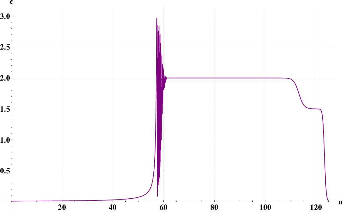
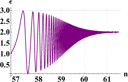
Inflation ends when $\epsilon(t_{e})=1$ , after which $\epsilon(t)$ oscillates between $\epsilon=0$ and $\epsilon=3$ , with constant amplitude and increasing frequency. A realistic model would couple the inflaton to normal matter, which would be heated by the inflaton’s kinetic energy to produce a radiation-dominated universe. At late times we want to reach the $\Lambda$ CDM model,

H^{2}=H_{0}^{2}\Bigl[\Omega_{r}(1\!+\!z)^{4}+\Omega_{m}(1\!+\!z)^{3}+\Omega_{\Lambda}\Bigr]\qquad,\qquad 1+z\equiv\frac{a_{0}}{a(t)}\;,

(40)

where the subscript $0$ represents the current time and the various parameters are [26],

H_{0}\simeq 67.3\,\frac{\rm km/s}{\rm Mpc}\quad,\quad\Omega_{r}\simeq\frac{\Omega_{m}}{3390}\quad,\quad\Omega_{m}\simeq 0.315\quad,\quad\Omega_{\Lambda}\simeq 0.685\;.

(41)

Refer to caption — Figure 1: The first plot shows first slow roll parameter $\epsilon$ over the full range of cosmic history. The second plot the interpolation (43) during reheating.

The first slow roll parameter of the $\Lambda$ CDM model is,

\epsilon_{\Lambda}(t)=\frac{2\Omega_{r}(1\!+\!z)^{4}+\frac{3}{2}\Omega_{m}(1\!+\!z)^{3}}{\Omega_{r}(1\!+\!z)^{4}+\Omega_{m}(1\!+\!z)^{3}+\Omega_{\Lambda}}\qquad,\qquad 1\!+\!z=\frac{a_{0}}{a(t)}\;.

(42)

Rather than devise a model of reheating, we have merely made an ad hoc interpolation of the first slow roll parameter between the scalar-driven result (38) and the $\Lambda$ CDM result (42),

\epsilon(t)=\frac{1}{2}\Bigl[1-\tanh(n\!-\!n_{\rm eq})\Bigr]\!\times\!\epsilon_{\varphi}(t)+\frac{1}{2}\Bigl[1+\tanh(n\!-\!n_{\rm eq})\Bigr]\!\times\!\epsilon_{\Lambda}(t)\;,

(43)

where $\epsilon_{\varphi}(t)$ and $\epsilon_{\Lambda}(t)\simeq 2$ were defined in expressions (38) and (42), respectively, $n$ is the number of e-foldings since the start of inflation at $t=t_{i}$ , $n\equiv\ln[a(t)/a(t_{i})]$ . Figure 1 shows the resulting geometry.

The e-folding $n_{\rm eq}=59.1$ at which scalar-driven inflation and the $\Lambda$ CDM model are equally represented was chosen for numerical convenience. Any value more than a few e-foldings after the end of inflation at $n_{e}\simeq 56.8$ could be used instead. The current time $t_{0}$ , corresponding to $n_{0}\simeq 123.9$ , is found by integrating expression (43) — using $\epsilon_{\Lambda}=2$ — from the end of inflation to a time $t_{\rm rad}$ a few e-foldings past $n=n_{\rm eq}$ . By that point the $\Lambda$ CDM geometry dominates, and we can assume its radiation-dominated form to write,

H(t_{\rm rad})=\frac{H(t_{e})}{1+H(t_{e})\int_{t_{e}}^{t_{\rm rad}}\!\!dt^{\prime}\,\epsilon(t^{\prime})}\equiv H_{0}\sqrt{\Omega_{r}}e^{2(n_{\rm rad}-n_{0})}\;.

(44)

We close by stressing that this geometry has been introduced merely to provide an explicit framework for comparing the exact numerical evolution of $\mathcal{A}(t,k)$ with the analytic approximations we shall develop in section 3. These analytic approximations have nothing to do with specific properties of our plausible geometry. In particular, they do not depend on inflation being supported by a scalar potential, much less the quadratic potential, nor do they depend on the initial value of this scalar, the constant $c$ , or the interpolation (43) between scalar-driven inflation and the $\Lambda$ CDM cosmology.

2.3 Dimensionless Variables

The variable $n\equiv\ln[a(t)/a_{i}]$ is preferable to $t$ , both because $n$ is dimensionless and because it is less sensitive to dramatic changes which take place in the time scale of events as inflation progresses. Derivatives obey,

\frac{d}{dt}=H\frac{d}{dn}\;,\;\frac{d^{2}}{dt^{2}}=H^{2}\Bigl[\frac{d^{2}}{dn^{2}}\!-\!\epsilon\frac{d}{dn}\Bigr]\;,\;\frac{d^{3}}{dt^{3}}=H^{3}\Bigl[\frac{d^{3}}{dn^{3}}\!-\!3\epsilon\frac{d^{2}}{dn^{2}}\!+\!(2\epsilon^{2}\!-\!\epsilon^{\prime})\frac{d}{dn}\Bigr].

(45)

Just as dots denote differentiation with respect to $t$ we use primes to stand for differentiation with respect to $n$ , except that a primed potential still represents its derivative with respect to the scalar. It is convenient to factor the dimensions out of the inflaton, the Hubble parameter and the inflaton potential,

\psi(n)\equiv\sqrt{8\pi G}\,\varphi(t)\quad,\quad\chi(n)\equiv\sqrt{8\pi G}\,H(t)\quad,\quad U(\psi)\equiv(8\pi G)^{2}V(\varphi)\;.

(46)

Of course the first slow roll parameter $\epsilon=-\chi^{\prime}/\chi$ is already dimensionless. Using these variables, and expressions (35-36), to solve for the geometrical quantities in terms of the scalar,

\chi^{2}=\frac{U}{3\!-\!\frac{1}{2}{\psi^{\prime}}^{2}}\qquad,\qquad\epsilon=\frac{1}{2}{\psi^{\prime}}^{2}\;.

(47)

We can also re-express the scalar evolution equation (37) as,

\psi^{\prime\prime}+(3\!-\!\epsilon)\psi^{\prime}+\frac{U^{\prime}(\psi)}{\chi^{2}}=0\qquad\Longrightarrow\qquad\psi^{\prime\prime}+\Bigl(3-\frac{1}{2}{\psi^{\prime}}^{2}\Bigr)\Bigl[\psi^{\prime}+\frac{U^{\prime}}{U}\Bigr]=0\;.

(48)

For the quadratic potential $U(\psi)=\frac{1}{2}c^{2}\psi^{2}$ we have chosen, the slow roll approximation gives,

\psi(n)\simeq\sqrt{\psi_{i}^{2}\!-\!4n}\quad,\quad\chi(n)\simeq\frac{c}{\sqrt{6}}\sqrt{\psi_{i}^{2}\!-\!4n}\quad,\quad\epsilon\simeq\frac{2}{\psi_{i}^{2}\!-\!4n}\;.

(49)

We scale out the dimensions of the wave number and the amplitude,

\kappa\equiv\sqrt{8\pi G}\,k\qquad,\qquad\alpha(n,\kappa)\equiv\frac{\mathcal{A}(t,k)}{\sqrt{8\pi G}}\;.

(50)

The 2nd order and 3rd order equations (32-33) become,

$\displaystyle 0$	$\displaystyle\!\!\!=\!\!\!$	$\displaystyle\alpha^{\prime\prime}-\frac{{\alpha^{\prime}}^{2}}{2\alpha}+(D\!-\!1\!-\!\epsilon)\alpha^{\prime}+\frac{2\kappa^{2}\alpha}{e^{2n}\chi^{2}}-\frac{e^{-2(D-1)n}}{2\chi^{2}\alpha}\;,\qquad$	(51)
$\displaystyle 0$	$\displaystyle\!\!\!=\!\!\!$	$\displaystyle\alpha^{\prime\prime\prime}+3(D\!-\!1\!-\!\epsilon)\alpha^{\prime\prime}+\Bigl[2(D\!-\!1\!-\!\epsilon)^{2}\!-\!\epsilon^{\prime}\Bigr]\alpha^{\prime}$	(52)
		$\displaystyle\hskip 213.39566pt+\frac{4\kappa^{2}\alpha^{\prime}}{e^{2n}\chi^{2}}+\frac{4(D\!-\!2)\kappa^{2}\alpha}{e^{2n}\chi^{2}}\;.\qquad$	(52)

The WKB form (27) implies initial conditions,

\alpha(0,\kappa)=\frac{1}{2\kappa}\quad,\quad\alpha^{\prime}(0,\kappa)=-\frac{(D\!-\!2)}{2\kappa}\quad,\quad\alpha^{\prime\prime}(0,\kappa)=\frac{(D\!-\!2)^{2}}{2\kappa}\;.

(53)

3 Approximating $\mathcal{A}(t,k)$

The purpose of this section is to develop analytic approximations for the amplitude $\mathcal{A}(t,k)$ according to where the wave number $k$ lies with respect to $H(t)a(t)$ . When $k=Ha$ the mode is said to experience horizon crossing. The section begins with a discussion of horizon crossing. We then give successive analytic approximations for ultraviolet modes which have never experienced horizon crossing, for modes which have experienced one crossing and for modes which have twice experienced crossing.

3.1 Horizon Crossing

Modes are said to be sub-horizon if $k>H(t)a(t)$ and super-horizon if $k<H(t)a(t)$ . We do not assume that the mode sums (28-31) run all the way down to $k=0$ , but rather that the far infrared portion is cut off for modes $k<k_{i}=H(t_{i})a(t_{i})$ which were super-horizon at the beginning of inflation. (Justified by pre-inflationary modes being less highly excited [27], or else by the spatial manifold being compact [28].) This means that all modes are initially sub-horizon and may, or may not, experience horizon crossing during the course of primordial inflation. Some of those modes which have experienced first horizon crossing may experience second crossing.

Figure 2 shows the evolution of the logarithm of $\chi(n)e^{n}=\sqrt{8\pi G}\times H(t)a(t)$ over the course of the plausible expansion history described in section 2.2.

We define the first horizon crossing time $t_{k}$ as the time when a mode with wave number $k$ intersects the left hand, rising portion of the curve, $k=a(t_{k})H(t_{k})$ . During primordial inflation the product $H(t)a(t)$ grows from $k_{i}$ and distinguishes modes which have experienced first horizon crossing from those which are still ultraviolet,

{\rm During\ Inflation}\qquad\Longrightarrow\qquad k_{i}<H(t)a(t)<\infty\;.

(54)

If $t_{e}$ represents the end of primordial inflation then, except for a brief oscillatory period during reheating, $H(t)a(t)$ falls off from $k_{e}\equiv H(t_{e})a(t_{e})$ and we can distinguish a 3rd class of modes — between the infrared and the ultraviolet — which have experienced 2nd horizon crossing,

{\rm After\ Inflation}\qquad\Longrightarrow\qquad k_{i}<H(t)a(t)<k_{e}<\infty\;.

(55)

In performing the mode sum (next section) it will be desirable to change variables from wave number $k$ to the first horizon crossing time $t_{k}$ ,

k=a(t_{k})H(t_{k})\qquad\Longrightarrow\qquad\frac{dk}{k}=[1\!-\!\epsilon(t_{k})]H(t_{k})dt_{k}\;.

(56)

It is also useful to have an expression for the time $t_{2}(t_{k})$ that a mode with first horizon crossing time experiences second horizon crossing,

k\equiv a(t_{k})H(t_{k})\equiv a\Bigl(t_{2}(t_{k})\Bigr)H\Bigl(t_{2}(t_{k})\Bigr)\;.

(57)

Figure 2 shows that this is a well-defined function, except for the late phase of cosmic acceleration, and the small oscillatory range during reheating. The inverse of $t_{2}(t_{1})$ is $t_{1}(t_{2})$ ,

t_{1}\Bigl(t_{2}(t)\Bigr)\equiv t\qquad\Longleftrightarrow\qquad t_{1}\Bigl(t_{2}(t)\Bigr)=t\;.

(58)

3.2 Before 1st Horizon Crossing

The dimensionless amplitude $\alpha(n,\kappa)=\mathcal{A}(t,k)/\sqrt{8\pi G}$ is not known for general $\epsilon$ but it is easy to develop an ultraviolet expansion which applies for $\kappa\gg e^{n}\chi(n)$ . To do this we make the definitions,

\alpha(n,\kappa)\equiv\frac{\gamma(n,\kappa)}{2\kappa e^{(D-2)n}}\qquad,\qquad\zeta(n,\kappa)\equiv\frac{\kappa}{e^{n}\chi(n)}\;,

(59)

and substitute into equation (51) to obtain,

\gamma^{\prime\prime}-\frac{{\gamma^{\prime}}^{2}}{2\gamma}+(1\!-\!\epsilon)\gamma^{\prime}-\frac{1}{2}(D\!-\!2)(D\!-\!2\epsilon)\gamma+2\zeta^{2}\Bigl(\gamma-\frac{1}{\gamma}\Bigr)=0\;.

(60)

Relation (60) gives an expansion for $\gamma(n,\kappa)$ in powers of $\zeta^{-2}$ , where the coefficients involve increasing numbers of derivatives of $\epsilon(n)$ ,

	$\displaystyle\gamma=1+\frac{(D\!-\!2)(D\!-\!2\epsilon)}{8\zeta^{2}}+\frac{3(D\!-\!2)(D\!-\!2\epsilon)(D\!-\!4\!+\!2\epsilon)(D\!+\!2\!-\!4\epsilon)}{128\zeta^{4}}+\dots$				(61)
			$\displaystyle\hskip 142.26378pt+\frac{(D\!-\!2)[(D\!+\!5\!-\!7\epsilon)\epsilon^{\prime}\!+\!\epsilon^{\prime\prime}]}{16\zeta^{4}}+O(\zeta^{-6})\;.\qquad$		(61)

Note that $\gamma=1$ is an exact solution for $D=2$ and/or for perfect radiation-domination ( $\epsilon=\frac{D}{2}$ ). Figure 3 compares the exact numerical evolution with the asymptotic series (including the $\zeta^{-2}$ contribution in (61) but not the $\zeta^{-4}$ term) for a mode which experiences horizon crossing at $n=10$ . It is not even possible to discern any difference between the two until after horizon crossing.

3.3 Between 1st and 2nd Horizon Crossing

Because ultraviolet divergences are associated with $k\rightarrow\infty$ , we can suspend dimensional regularization for modes which have experienced first horizon crossing. If the modes have not yet experienced second horizon crossing then the last two terms of equation (32) are negligible and we see that $\mathcal{A}(t,k)$ approaches a constant. This constant is approximately [25],

t>t_{k}\Longrightarrow\mathcal{A}(t,k)\simeq\frac{H^{2}(t_{k})C(\epsilon_{k})}{2k^{3}}\Biggl\{1+O\Bigl(\frac{k^{2}}{a^{2}(t)H^{2}(t)}\Bigr)\Biggr\}\;,

(62)

where the function $C(\epsilon)$ is,

C(\epsilon)\equiv\frac{1}{\pi}\Gamma^{2}\Bigl(\frac{1}{2}+\frac{1}{1\!-\!\epsilon}\Bigr)\Bigl[2(1\!-\!\epsilon)\Bigr]^{\frac{2}{1-\epsilon}}\;.

(63)

Expressions (62-63) give the freeze-in amplitude to all orders in the slow roll approximation.

The solid green line in Figure 3 gives the logarithm of the freeze-in amplitude (62-63) for a mode which experiences horizon crossing at $n=10$ . It is difficult to detect any difference between it and the numerical solution (in dashed yellow) after horizon crossing. We possess good analytical approximations for additional, nonlocal contributions to the freeze-in amplitude, but these are very small unless the first slow roll parameter varies wildly near the time of first horizon crossing [29].

3.4 After 2nd Horizon Crossing

After 2nd horizon crossing the time dependence of the WKB form (27), applies but starting with $\dot{\mathcal{A}}(t,k)=0$ at $t=t_{2}(t_{k})$ from the freeze-in amplitude (62-63),

t>t_{2}(t_{k})\Longrightarrow\mathcal{A}(t,k)\simeq\frac{H^{2}(t_{k})C(\epsilon(t_{k}))}{2k^{3}}\!\times\!\Bigl[\frac{a(t_{2}(t_{k}))}{a(t)}\Bigr]^{2}\!\cos^{2}\Biggl[\int_{t_{2}(t_{k})}^{t}\!\!\!\!\!\!\!\!dt^{\prime}\frac{k}{a(t^{\prime})}\Biggr].

(64)

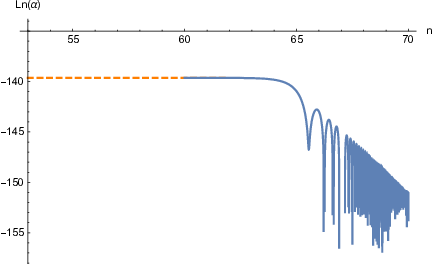
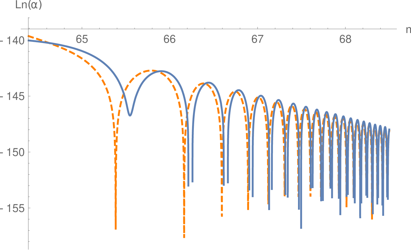
Figure 4 compares the exact numerical evolution (on the left) with the analytic approximation (on the right) for a mode which experiences first horizon crossing at $n=50$ and second horizon crossing at $n\simeq 64.5$ . The agreement is quite good, except for the first oscillation which suffers from the usual inaccuracy when the WKB frequency vanishes. Because the rapid oscillations of the cosine-squared average to $\frac{1}{2}$ inside the mode sum, the important part is the $1/a^{2}(t)$ damping.

4 Results for $A(t)$

The purpose of this section is to insert the approximate results (59-61), (62-63) and (64) for the amplitude $\mathcal{A}(t,k)$ into the mode sum (28) for $A(t)$ . We begin with the case of primordial inflation, during which the mode sum can be decomposed into before and after first horizon crossing. After the end of inflation the modes which have most recently experienced 1st crossing experience 2nd crossing, which gives a third range of modes between the first two. We then consider what the expectation value of the scalar propagator might be for a general metric. The section closes with a comment on why we do not employ the instantaneously constant $\epsilon$ approximation.

4.1 During Primordial Inflation

Because the amplitude $\mathcal{A}(t,k)$ depends on the wave vector $\vec{k}$ only through its magnitude, we can perform the angular integrations in the mode sum (28),

A(t)=\frac{2}{\Gamma(\frac{D-1}{2})(4\pi)^{\frac{D-1}{2}}}\!\int_{k_{i}}^{\infty}\!\!\!\!dk\,k^{D-2}\mathcal{A}(t,k)\;.

(65)

Note that the lower limit of the mode sum has been cut off at the wave number $k_{i}=H(t_{i})a(t_{i})$ which is just crossing the horizon at the start of inflation. During inflation we distinguish between ultraviolet modes ( $H(t)a(t)<k<\infty$ ), which have not yet experienced first horizon crossing, and infrared ones ( $k_{i}<k<H(t)a(t)$ ), which have already done so,

\int_{k_{i}}^{\infty}\!\!\!\!dk=\int_{Ha}^{\infty}\!\!\!\!\!\!dk+\int_{k_{i}}^{Ha}\!\!\!\!\!\!dk\;.

(66)

Figure 3 shows that we only need the first two terms of the ultraviolet expansion (59-61) to accurately describe $\mathcal{A}(t,k)$ right up to the point of first horizon crossing, and that the freeze-in amplitude (62-63) is valid afterwards. Making the appropriate substitutions in the mode sum gives,

	$\displaystyle A(t)\simeq\frac{2}{\Gamma(\frac{D-1}{2})(4\pi)^{\frac{D-1}{2}}}\int_{aH}^{\infty}\!\!\frac{dkk^{D-2}}{2ka^{D-2}}\Biggl\{1+\frac{(D\!-\!2)(D\!-\!2\epsilon)}{8}\frac{a^{2}H^{2}}{k^{2}}\Biggr\}$				(67)
			$\displaystyle\hskip 199.16928pt+\frac{1}{2\pi^{2}}\!\!\int_{a_{i}H_{i}}^{aH}\!\!\!\!dk\,k^{2}\frac{H^{2}(t_{k})C(\epsilon_{k})}{2k^{3}}\;.\qquad$		(67)

Note that we have suspended dimensional regularization on the infrared portion of the mode sum.

Under the rules of dimensional regularization, any $D$ -dependent power of infinity (or zero) vanishes,

	$\displaystyle\int_{aH}^{\infty}\!\!\!\!dk\,k^{D-3}$	$\displaystyle=$	$\displaystyle\frac{k^{D-2}}{D-2}\Bigl\|_{aH}^{\infty}=-\frac{(aH)^{D-2}}{D-2}\longrightarrow-\frac{1}{2}(aH)^{2}\;,$		(68)
	$\displaystyle\int_{aH}^{\infty}\!\!\!\!dk\,k^{D-5}$	$\displaystyle=$	$\displaystyle\frac{k^{D-4}}{D-4}\Bigl\|_{aH}^{\infty}=-\frac{(aH)^{D-4}}{D-4}\;.$		(69)

It is also convenient to change variables from $k$ to the time $t_{k}$ of first horizon crossing for the sum over modes which have experienced first horizon crossing,

k=H(t_{k})a(t_{k})\qquad\Longrightarrow\qquad\frac{dk}{k}=[1\!-\!\epsilon(t_{k})]H(t_{k})dt_{k}\;.

(70)

Our final result for $A(t)$ is,

	$\displaystyle A(t)\simeq-\frac{1}{8}\Bigl(\frac{D\!-\!2}{D\!-\!4}\Bigr)\frac{[D\!-\!2\epsilon(t)]H^{D-2}(t)}{\Gamma(\frac{D-1}{2})(4\pi)^{\frac{D-1}{2}}}-\frac{H^{2}(t)}{8\pi^{2}}$				(71)
			$\displaystyle\hskip 165.02606pt+\frac{1}{4\pi^{2}}\!\!\int_{t_{i}}^{t}\!\!\!\!dt^{\prime}H^{3}(t^{\prime})\Bigl[1\!-\!\epsilon(t^{\prime})\Bigr]C\Bigl(\epsilon(t^{\prime})\Bigr)\;.\qquad$		(71)

It is worth noting that the divergent first term of (71) is proportional to the Ricci scalar $R(t)=(D-1)[D-2\epsilon(t)]H^{2}(t)$ .

4.2 After Primordial Inflation

Although expression (65) is generally valid, after the end of inflation $a(t)H(t)$ falls off and the larger $k$ modes which had experienced first horizon crossing undergo a second horizon crossing. If the end of inflation occurs at $t_{e}$ then the last mode which experiences first horizon crossing is $k_{e}=a(t_{e})H(t_{e})$ and we must distinguish between ultraviolet modes ( $k_{e}<k<\infty$ ) which never experienced horizon crossing, intermediate modes ( $a(t)H(t)<k<k_{e}$ ) which have undergone both first and second crossing, and infrared modes ( $k_{i}<k<a(t)H(t)$ ) which are still super-horizon,

\int_{k_{i}}^{\infty}\!\!\!\!dk=\int_{k_{e}}^{\infty}\!\!\!\!\!\!dk+\int_{Ha}^{k_{e}}\!\!\!\!\!\!dk+\int_{k_{i}}^{Ha}\!\!\!\!\!\!dk\;.

(72)

The ultraviolet integrations are somewhat different from before,

	$\displaystyle\int_{k_{e}}^{\infty}\!\!\!\!dk\,k^{D-3}$	$\displaystyle=$	$\displaystyle\frac{k^{D-2}}{D-2}\Bigl\|_{k_{e}}^{\infty}=-\frac{k_{e}^{D-2}}{D-2}\longrightarrow-\frac{1}{2}k_{e}^{2}\;,$		(73)
	$\displaystyle\int_{k_{e}}^{\infty}\!\!\!\!dk\,k^{D-5}$	$\displaystyle=$	$\displaystyle\frac{k^{D-4}}{D-4}\Bigl\|_{k_{e}}^{\infty}=-\frac{k_{e}^{D-4}}{D-4}\longrightarrow-\frac{[aH]^{D-4}}{D-4}-\ln\Bigl[\frac{k_{e}}{aH}\Bigr]\;.$		(74)

We convert the intermediate mode sum from $k$ to the time of second crossing,

$\displaystyle\frac{1}{4\pi^{2}}\!\int_{aH}^{k_{e}}\!\!\frac{dk}{k}\,H^{2}(t_{k})C\Bigl(\epsilon(t_{k})\Bigr)\!\times\!\Bigl[\frac{a(t_{2}(t_{k}))}{a(t)}\Bigr]^{2}\cos^{2}\Bigl[\int_{t_{2}(t_{k})}^{t}\!\!\!\!\!\!\!\!dt^{\prime\prime}\frac{k}{a(t^{\prime\prime})}\Bigr]$		(75)
	$\displaystyle\hskip 0.0pt=\frac{1}{4\pi^{2}a^{2}(t)}\!\int_{t_{e}}^{t}\!\!\!dt^{\prime}[\epsilon(t^{\prime})\!-\!1]H(t^{\prime})a^{2}(t^{\prime})\cos^{2}\Bigl[\int_{t^{\prime}}^{t}\!\!\frac{kdt^{\prime\prime}}{a(t^{\prime\prime})}\Bigr]\!\times\!H^{2}(t_{1})C\Bigl(\!\epsilon(t_{1})\!\Bigr),\qquad$	(75)
	$\displaystyle\hskip 0.0pt\simeq\frac{1}{8\pi^{2}a^{2}(t)}\!\int_{t_{e}}^{t}\!\!\!dt^{\prime}[\epsilon(t^{\prime})\!-\!1]H(t^{\prime})a^{2}(t^{\prime})\!\times\!H^{2}(t_{1})C\Bigl(\epsilon(t_{1})\Bigr).\qquad$	(76)

The rapid oscillations evident in Figure 4 justify replacing $\cos^{2}$ by $\frac{1}{2}$ . Super-horizon modes contribute the same as for (71) except that the upper limit is $t_{2}(t_{i})$ . Our final result for $A(t)$ is,

$\displaystyle A(t)\simeq-\frac{1}{8}\Bigl(\frac{D\!-\!2}{D\!-\!4}\Bigr)\frac{[D\!-\!2\epsilon(t)]H^{D-2}(t)}{\Gamma(\frac{D-1}{2})(4\pi)^{\frac{D-1}{2}}}-\frac{[2\!-\!\epsilon(t)]H^{2}(t)}{8\pi^{2}}\ln\Bigl[\frac{k_{e}}{a(t)H(t)}\Bigr]$		(77)
	$\displaystyle\hskip 0.0pt-\frac{1}{8\pi^{2}}\!\times\!\Bigl[\frac{k_{e}}{a(t)}\Bigr]^{2}+\frac{1}{8\pi^{2}a^{2}(t)}\!\int_{t_{e}}^{t}\!\!\!dt^{\prime}[\epsilon(t^{\prime})\!-\!1]H(t^{\prime})a^{2}(t^{\prime})\!\times\!H^{2}(t_{1})C\Bigl(\epsilon(t_{1})\Bigr)$
	$\displaystyle\hskip 128.0374pt+\frac{1}{4\pi^{2}}\!\!\int_{t}^{t_{2}(t_{i})}\!\!\!\!\!\!\!\!\!\!\!\!dt^{\prime}[\epsilon(t^{\prime})\!-\!1]H(t^{\prime})\!\times\!H^{2}(t_{1})C\Bigl(\epsilon(t_{1})\Bigr).\qquad$

4.3 General Metric Form

The expectation value of $\phi^{2}$ must be a scalar functional of the metric. We only need it for the class of metrics (1) in order to model cosmology, however, describing changes to the force of gravity requires a more general class of metrics. And it is worth mentioning that 1-loop computations on de Sitter background indicate that the force of gravity can experience nonperturbatively strong corrections from inflationary scalars [8] and gravitons [11].

Expressions (71) and (77) make it plain that the divergence in $i\Delta(x;x^{\prime})$ is proportional to the Ricci scalar. The old result (21) of Dolgov and Pellicia [23] suggests that we try to model the finite, nonlocal part as the inverse of the covariant d’Alembertian,

\kern 1.0pt\vbox{\hrule height=1.2pt\hbox{\vrule width=1.2pt\hskip 3.0pt\vbox{\vskip 6.0pt}\hskip 3.0pt\vrule width=0.6pt}\hrule height=0.6pt}\kern 1.0pt=-\Bigl(\frac{d}{dt}+3H\Bigr)\frac{d}{dt}\;,

(78)

acting on some curvature-squared. From the nonlocal part of $A(t)$ during inflation (71) we find,

	$\displaystyle\kern 1.0pt\vbox{\hrule height=1.2pt\hbox{\vrule width=1.2pt\hskip 3.0pt\vbox{\vskip 6.0pt}\hskip 3.0pt\vrule width=0.6pt}\hrule height=0.6pt}\kern 1.0pt\!\int_{t_{i}}^{t}\!\!\!\!dt^{\prime}H^{3}(1\!-\!\epsilon)C(\epsilon)=-\Bigl(\frac{d}{dt}+3H\Bigr)\Bigl\{H^{3}(1\!-\!\epsilon)C(\epsilon)\Bigr\}\;,$				(79)
			$\displaystyle\hskip 85.35826pt=-3H^{4}(1\!-\!\epsilon)^{2}C(\epsilon)+H^{3}\Bigl[C(\epsilon)+(1\!-\!\epsilon)C^{\prime}(\epsilon)\Bigr]\dot{\epsilon}\;.\qquad$		(80)

Trying to understand (80) as something quadratic in the curvature is challenging because of the complicated function $C(\epsilon)$ given in expression (63). However, it was never realistic to devise a simple model for the full nonlocal part; what we seek instead is a reasonable approximation. In this regard it is worth noting that the function $C(\epsilon)$ is not far off from $1-\epsilon$ , as shown in Figure 5.

If we employ $C(\epsilon)\simeq 1-\epsilon$ , and neglect the $\dot{\epsilon}$ terms in (80), it follows that the quadratic curvature we seek is approximately,

\kern 1.0pt\vbox{\hrule height=1.2pt\hbox{\vrule width=1.2pt\hskip 3.0pt\vbox{\vskip 6.0pt}\hskip 3.0pt\vrule width=0.6pt}\hrule height=0.6pt}\kern 1.0pt\Biggl\{\frac{1}{4\pi^{2}}\!\int_{t_{i}}^{t}\!\!\!\!dt^{\prime}H^{3}(1\!-\!\epsilon)C(\epsilon)\Biggr\}\simeq-\frac{3}{4\pi^{2}}\,H^{4}(1\!-\!\epsilon)^{3}

(81)

Specializing the Riemann tensor and its contractions to the cosmological background (1) gives,

	$\displaystyle R^{0}_{~i0j}=(1\!-\!\epsilon)H^{2}g_{ij}$	,	$\displaystyle R^{i}_{~jk\ell}=H^{2}\Bigl(\delta^{i}_{~k}g_{j\ell}\!-\!\delta^{i}_{~\ell}g_{jk}\Bigr),\qquad$		(82)
	$\displaystyle R_{00}=-3(1\!-\!\epsilon)H^{2}$	,	$\displaystyle R_{ij}=(3\!-\!\epsilon)H^{2}g_{ij}\;.\qquad$		(83)

Had there been only two factors of $(1-\epsilon)$ , instead of three, we would have recognized two factors of $R_{00}$

\kern 1.0pt\vbox{\hrule height=1.2pt\hbox{\vrule width=1.2pt\hskip 3.0pt\vbox{\vskip 6.0pt}\hskip 3.0pt\vrule width=0.6pt}\hrule height=0.6pt}\kern 1.0pt\Biggl\{\frac{1}{4\pi^{2}}\!\int_{t_{i}}^{t}\!\!\!\!dt^{\prime}H^{3}(1\!-\!\epsilon)C(\epsilon)\Biggr\}\simeq-\frac{R_{00}^{2}}{12\pi^{2}}\;.

(84)

This is curiously similar to the nonlocal invariant $Y[g]$ which was employed [30, 31, 32] to construct a relativistic, purely metric realization of Milgrom’s Modified Newtonian Gravity (MOND) [33, 34]. However, the extra factor of $1-\epsilon$ spoils this correspondence. Nor does the $R_{00}^{2}$ form extend to the post-inflationary regime, during which no new modes experience first horizon crossing and the only weak time dependence derives from the $1/a^{2}(t)$ redshift of modes which have undergone second horizon crossing.

4.4 Instantaneously Constant $\epsilon$ Approximation

When the first slow roll parameter is constant the amplitude $\alpha(n,\kappa)$ turns out to be a simple factor times the norm-squared of a Hankel function of the first kind. We define the $\alpha_{1}$ approximation by replacing the constant first slow roll parameter of this solution with $\epsilon(n)$ ,

\alpha_{1}(n,\kappa)\equiv\frac{1}{2\kappa e^{(D-2)n}}\!\times\!\frac{\pi}{2}\!\times\!z(n,\kappa)\!\times\!\Bigl|H^{(1)}_{\nu(n)}\Bigl(z(n,\kappa)\Bigr)\Bigr|^{2}\equiv\frac{\gamma_{1}(n,\kappa)}{2\kappa e^{(D-2)n}}\;.

(85)

Here the argument $z(n,\kappa)$ and the index $\nu(n)$ are,

z(n,\kappa)\equiv\frac{\kappa e^{-n}}{(1\!-\!\epsilon)\chi}=\frac{\zeta(n,\kappa)}{1\!-\!\epsilon}\qquad,\qquad\nu(n)\equiv\frac{(D\!-\!1\!-\!\epsilon)}{2(1\!-\!\epsilon)}.

(86)

The large $z$ asymptotic form of the Hankel function implies,

\gamma_{1}=\frac{\pi z}{2}\Bigl|H^{(1)}_{\nu}(z)\Bigr|^{2}=1+\frac{(\nu^{2}\!-\!\frac{1}{4})}{2z^{2}}+\frac{3(\nu^{2}\!-\!\frac{1}{4})(\nu^{2}\!-\!\frac{9}{4})}{8z^{4}}+O(z^{-6})\;.

(87)

From the definitions (86) of $z(n,\kappa)$ and $\nu(n)$ we infer the relations,

	$\displaystyle\frac{(\nu^{2}\!-\!\frac{1}{4})}{z^{2}}$	$\displaystyle\!\!\!=\!\!\!$	$\displaystyle\frac{(D\!-\!2)(D\!-\!2\epsilon)}{4\zeta^{2}}\;,\qquad$		(88)
	$\displaystyle\frac{(\nu^{2}\!-\!\frac{9}{4})}{z^{2}}$	$\displaystyle\!\!\!=\!\!\!$	$\displaystyle\frac{(D\!-\!4\!+\!2\epsilon)(D\!+\!2\!-\!4\epsilon)}{4\zeta^{2}}\;.\qquad$		(89)

It follows that the large $z$ expansion of $\gamma_{1}$ gives all the terms on the first line of (61),

\gamma_{1}=1\!+\!\frac{(D\!-\!2)(D\!-\!2\epsilon)}{8\zeta^{2}}\!+\!\frac{3(D\!-\!2)(D\!-\!2\epsilon)(D\!-\!4\!+\!2\epsilon)(D\!+\!2\!-\!4\epsilon)}{128\zeta^{4}}+O(\zeta^{-6})\;.

(90)

However, the ultraviolet expansion of $\gamma_{1}(n,\kappa)$ fails to recover the terms involving derivatives of $\epsilon$ on the second line of (61). Therefore, the instantaneously constant $\epsilon$ approximation reproduces the ultraviolet divergences of $A(t)$ and $B_{\mu}(t)$ , but it misses some divergences in $C_{0}(t)$ and $\overline{C}(t)$ .

The instantaneously constant $\epsilon$ approximation also gives misleading results for the infrared. To see this we evaluate the coincidence limit of the propagator in this approximation [35],

i\Delta_{1}(x;x)=\frac{[(1\!-\!\epsilon)H]^{D-2}}{(4\pi)^{\frac{D}{2}}}\frac{\Gamma(2\!-\!\frac{D}{2})}{\frac{D}{2}\!-\!1}\frac{\Gamma(\frac{D-1}{2}\!+\!\nu)\Gamma(\frac{D-1}{2}\!-\!\nu)}{\Gamma(\frac{1}{2}\!+\!\nu)\Gamma(\frac{1}{2}\!-\!\nu)}\;.

(91)

The complicated ratio of Gamma functions in (91) can be expanded around $\delta\equiv 4-D$ ,

	$\displaystyle\frac{\Gamma(\frac{D-1}{2}\!+\!\nu)\Gamma(\frac{D-1}{2}\!-\!\nu)}{\Gamma(\frac{1}{2}\!+\!\nu)\Gamma(\frac{1}{2}\!-\!\nu)}=\Bigl[\Bigl(\frac{D\!-\!3}{2}\Bigr)^{2}\!-\!\nu^{2}\Bigr]\!\times\!\frac{\Gamma(\frac{1}{2}\!+\!\nu\!-\!\frac{\delta}{2})\Gamma(\frac{1}{2}\!-\!\nu)\!-\!\frac{\delta}{2})}{\Gamma(\frac{1}{2}\!+\!\nu)\Gamma(\frac{1}{2}\!-\!\nu)}\;,$				(92)
			$\displaystyle\hskip-14.22636pt=-\frac{(D\!-\!2)(2\!-\!\epsilon)[2\!+\!(D\!-\!4)\epsilon]}{4(1\!-\!\epsilon)^{2}}\Biggl\{1\!-\!\psi\Bigl(\frac{1}{2}\!+\!\nu\Bigr)\frac{\delta}{2}\!-\!\psi\Bigl(\frac{1}{2}\!-\!\nu\Bigr)\frac{\delta}{2}+O(\delta^{2})\Biggr\}.\qquad$		(93)

Note the unphysical poles in the finite parts,

	$\displaystyle\epsilon=1-\frac{1}{N}$	$\displaystyle\Longrightarrow$	$\displaystyle\psi\Bigl(\frac{1}{2}-\nu\Bigr)\longrightarrow\pm\infty\;,\qquad$		(94)
	$\displaystyle\epsilon=1+\frac{1}{N+1}$	$\displaystyle\Longrightarrow$	$\displaystyle\psi\Bigl(\frac{1}{2}+\nu\Bigr)\longrightarrow\pm\infty\;.\qquad$		(95)

These poles arise because the instantaneously constant $\epsilon$ mode sum contains infrared divergences for all values in the range $0\leq\epsilon\leq\frac{3}{2}$ [36]. However, in most cases the divergences are of the power-law type which dimensional regularization automatically subtracts. For the special values (94-95) one of the infrared divergences happens to become logarithmic, at which point dimensional regularization registers it as a divergence at $D=4$ [35].

The infrared divergences (94-95) are unphysical for two reasons. First, the actual amplitude freezes in to a constant (62) which depends on the first slow roll parameter at horizon crossing, $\epsilon(n_{k})$ , rather than the evolving value $\epsilon(n)$ . Second, modes which were already super-horizon at the beginning of inflation ( $k<k_{i}$ ) would not have experienced the evolution necessary to reach their freeze-in amplitudes (62). These small modes can either be assumed to exist in some less infrared singular state [27], or else they can be discarded altogether, which would pertain if the spatial manifold were compact [28].

Although the infrared divergences (94-95) can be repaired by changing the mode sum [35], their presence indicates a profound problem with the instantaneously constant $\epsilon$ approximation. It seems best to avoid the approximation altogether, in spite of the fact that it was employed in similar studies of coincident inflationary propagators [37, 38, 39]. The key difference between those cases and this one is that nonzero masses protected the mode sum from infrared divergences.

5 Determining $B_{\mu}(t)$ , $C_{0}(t)$ and $\overline{C}(t)$

The purpose of this section is to use approximations (71) and (77) for $A(t)$ to infer approximations for $B_{\mu}(t)$ , $C_{0}(t)$ and $\overline{C}(t)$ . We begin by discussing the generic procedure for reconstructing $C_{0}(t)$ and $\overline{C}(t)$ from $A(t)$ . Then approximate results are derived for $B_{\mu}(t)$ , $C_{0}(t)$ and $\overline{C}(t)$ , first during inflation and then after the end of inflation.

5.1 Generic Considerations for $C_{0}(t)$ and $\overline{C}(t)$

The Introduction defined two linear combinations of $C_{0}$ and $\overline{C}$ ,

\Biggl\{\begin{matrix}C_{A}\equiv&-C_{0}+(D\!-\!1)\overline{C}\\ C_{B}\equiv&C_{0}+\overline{C}\end{matrix}\Biggr\}\quad\Longleftrightarrow\quad\Biggl\{\begin{matrix}C_{0}=&-\frac{1}{D}C_{A}+(\frac{D-1}{D})C_{B}\\ \overline{C}=&\frac{1}{D}C_{A}+\frac{1}{D}C_{B}\end{matrix}\Biggr\}.

(96)

Relation (21) gives $C_{A}$ in terms of $\kern 1.0pt\vbox{\hrule height=1.2pt\hbox{\vrule width=1.2pt\hskip 3.0pt\vbox{\vskip 6.0pt}\hskip 3.0pt\vrule width=0.6pt}\hrule height=0.6pt}\kern 1.0ptA$ ,

C_{A}(t)=-\frac{1}{2}\Bigl[\ddot{A}(t)+(D\!-\!1)H(t)\dot{A}(t)\Bigr]\;.

(97)

The other linear combination derives from conservation of the scalar stress tensor (24),

2\Bigl[\frac{d}{dt}+DH\Bigr]C_{B}=-\Bigl(\frac{D\!-\!2}{D\!-\!1}\Bigr)\dot{C}_{A}=\frac{1}{2}\Bigl(\frac{D\!-\!2}{D\!-\!1}\Bigr)\Bigl[\dddot{A}+(D\!-\!1)H\ddot{A}-(D\!-\!1)\epsilon H^{2}\dot{A}\Bigr]\;.

(98)

It is desirable to extract a factor of $(\frac{d}{dt}+DH)$ from the right hand side of (98) as much as possible,

\dddot{A}+(D\!-\!1)H\ddot{A}-(D\!-\!1)\epsilon H^{2}\dot{A}=\Bigl[\frac{d}{dt}+DH\Bigr]\Bigl[\ddot{A}-H\dot{A}\Bigr]+D(1\!-\!\epsilon)H^{2}\dot{A}\;.

(99)

Hence we can write,

	$\displaystyle C_{B}(t)=\frac{1}{4}\Bigl(\frac{D\!-\!2}{D\!-\!1}\Bigr)\Bigl[\ddot{A}(t)-H(t)\dot{A}(t)\Bigr]$				(100)
			$\displaystyle\hskip 99.58464pt+\frac{D(D\!-\!2)}{4(D\!-\!1)a^{D}(t)}\int_{t_{i}}^{t}\!\!\!\!dt^{\prime}\,a^{D}(t^{\prime})H^{2}(t^{\prime})[1\!-\!\epsilon(t^{\prime})]\dot{A}(t^{\prime})\;.\qquad$		(100)

A special case is the divergent part of $A(t)$ , which we see from (71) and (77) takes the form of $[D-2\epsilon]H^{D-2}$ . For this dependence, the final term of (99) allows another factor of $(\frac{d}{dt}+DH)$ to be extracted, up to a remainder proportional to $(D-4)$ ,

	$\displaystyle D(1\!-\!\epsilon)H^{2}\frac{d}{dt}\Bigl[(D\!-\!2\epsilon)H^{D-2}\Bigr]$				(101)
			$\displaystyle\hskip 14.22636pt=\Bigl[\frac{d}{dt}+DH\Bigr]\Bigl[-(D\!-\!2)\epsilon(D\!-\!2\epsilon)H^{D}\Bigr]+(D\!-\!4)\epsilon^{\prime}(D\!-\!2\epsilon)H^{D+1}\;.\qquad$		(101)

Relation (101) guarantees that the divergent parts of $C_{0}(t)$ and $\overline{C}(t)$ are local,

	$\displaystyle{C_{0}}_{\rm div}$	$\displaystyle\!\!\!=\!\!\!$	$\displaystyle\frac{1}{4}\Bigl\{\ddot{A}_{\rm div}+H\dot{A}_{\rm div}-\frac{(D\!-\!2)^{2}}{D}\,\epsilon H^{2}A_{\rm div}\Bigr\}\;,\qquad$		(102)
	$\displaystyle{\overline{C}}_{\rm div}$	$\displaystyle\!\!\!=\!\!\!$	$\displaystyle-\frac{1}{4(D\!-\!1)}\Bigl\{\ddot{A}_{\rm div}+(2D\!-\!3)H\dot{A}_{\rm div}+\frac{(D\!-\!2)^{2}}{D}\,\epsilon H^{2}A_{\rm div}\Bigr\}\;.\qquad$		(103)

The divergence structure (102-103) is consistent with an $R^{2}$ counterterm,

\Delta\mathcal{L}=\alpha R^{2}\sqrt{-g}\qquad\Longrightarrow\qquad\Delta T_{\mu\nu}=2\alpha\Bigl[R_{\mu\nu}-\frac{1}{4}g_{\mu\nu}R+g_{\mu\nu}\kern 1.0pt\vbox{\hrule height=1.2pt\hbox{\vrule width=1.2pt\hskip 3.0pt\vbox{\vskip 6.0pt}\hskip 3.0pt\vrule width=0.6pt}\hrule height=0.6pt}\kern 1.0pt-D_{\mu}D_{\nu}\Bigr]R\;.

(104)

The induced change in $C_{\mu\nu}$ is,

\Delta C_{\mu\nu}=\Delta T_{\mu\nu}-\frac{g_{\mu\nu}g^{\rho\sigma}T_{\rho\sigma}}{D\!-\!2}=2\alpha\Bigl[R_{\mu\nu}-\frac{g_{\mu\nu}R}{2(D\!-\!2)}-\frac{g_{\mu\nu}\kern 1.0pt\vbox{\hrule height=1.2pt\hbox{\vrule width=1.2pt\hskip 3.0pt\vbox{\vskip 6.0pt}\hskip 3.0pt\vrule width=0.6pt}\hrule height=0.6pt}\kern 1.0pt}{D\!-\!2}-D_{\mu}D_{\nu}\Bigr]R\;.

(105)

Using the $D$ -dimensional relations $R_{00}=-(D-1)(1-\epsilon)H^{2}$ and $R_{ij}=(D-1-\epsilon)H^{2}g_{ij}$ , we find the time-time and space-space components,

	$\displaystyle\Delta C_{00}$	$\displaystyle\!\!\!=\!\!\!$	$\displaystyle-2\alpha\Bigl(\frac{D\!-\!1}{D\!-\!2}\Bigr)\Bigl[\Bigl(\frac{D\!-\!4}{2}\Bigr)H^{2}-(D\!-\!3)\epsilon H^{2}+\frac{d^{2}}{dt^{2}}+H\frac{d}{dt}\Bigr]R\;,\qquad$		(106)
	$\displaystyle\Delta\overline{C}$	$\displaystyle\!\!\!=\!\!\!$	$\displaystyle\frac{2\alpha}{D\!-\!2}\Bigl[\frac{(D\!-\!1)(D\!-\!4)}{2}H^{2}+\epsilon H^{2}+\frac{d^{2}}{dt^{2}}+(2D\!-\!3)H\frac{d}{dt}\Bigr]R\;.\qquad$		(107)

Comparison between expressions (102-103) and (106-107) implies that the divergences can be canceled by,

\alpha=-\frac{1}{64}\Bigl(\frac{D\!-\!2}{D\!-\!1}\Bigr)^{2}\frac{1}{\Gamma(\frac{D-1}{2})(4\pi)^{\frac{D-1}{2}}}\times\frac{\mu^{D-4}}{D\!-\!4}\;,

(108)

where $\mu$ is the mass scale of dimensional regularization.

5.2 During Primordial Inflation

From expression (71) we can identify divergent and finite parts of $A(t)$ during inflation,

	$\displaystyle A_{\rm div}$	$\displaystyle\!\!\!=\!\!\!$	$\displaystyle-\frac{1}{8}\Bigl(\frac{D\!-\!2}{D\!-\!4}\Bigr)\frac{[D\!-\!2\epsilon(t)]H^{D-2}(t)}{\Gamma(\frac{D-1}{2})(4\pi)^{\frac{D-1}{2}}}\;,$		(109)
	$\displaystyle A_{\rm fin}$	$\displaystyle\!\!\!=\!\!\!$	$\displaystyle-\frac{H^{2}(t)}{8\pi^{2}}+\frac{1}{4\pi^{2}}\!\!\int_{t_{i}}^{t}\!\!\!\!dt^{\prime}H^{3}(t^{\prime})\Bigl[1\!-\!\epsilon(t^{\prime})\Bigr]C\Bigl(\epsilon(t^{\prime})\Bigr)\;.$		(110)

An important derived quantity is the finite residual at the end of relation (101),

\lim_{D\rightarrow 4}(D\!-\!4)\epsilon^{\prime}H^{3}A_{\rm div}=-\frac{H^{5}}{8\pi^{2}}(2\!-\!\epsilon)\epsilon^{\prime}\;.

(111)

Another key quantity is the first time derivative of the finite part,

\dot{A}_{\rm fin}=\frac{H^{3}}{4\pi^{2}}-\frac{H^{3}}{4\pi^{2}}(1\!-\!\epsilon)\Bigl(1\!-\!C(\epsilon)\Bigr)\;.

(112)

Our result for $B_{\mu}(t)$ involves (109) and (112),

B_{\mu}=\frac{1}{2}\Bigl\{\dot{A}_{\rm div}+\dot{A}_{\rm fin}\Bigr\}\delta^{0}_{~\mu}\;.

(113)

Taking $\epsilon=0$ in (113) agrees with the known de Sitter limit (19).

We have already derived results (102)-103) for the divergent parts of $C_{0}(t)$ and $\overline{C}(t)$ . To get the finite parts we must first derive the finite parts of $C_{A}(t)$ and $C_{B}(t)$ . The first of these is,

{C_{A}}_{\rm fin}=-\frac{1}{2}\Bigl(\frac{d}{dt}+3H\Bigr)\dot{A}_{\rm fin}\;.

(114)

To get the finite part of $C_{B}$ it is best to extract a factor of $(\frac{d}{dt}+4H)$ from $4(1-\epsilon)H^{2}$ times the first term of (112),

4(1\!-\!\epsilon)H^{2}\dot{A}_{\rm fin}=\Bigl(\frac{d}{dt}+4H\Bigr)\Bigl\{\frac{H^{4}}{4\pi^{2}}\Bigr\}-\frac{H^{5}}{8\pi^{2}}\!\times\!8(1\!-\!\epsilon)^{3}[1\!-\!C(\epsilon)]\;.

(115)

It follows that the finite part of $C_{B}$ is,

	$\displaystyle{C_{B}}_{\rm fin}=\frac{1}{6}\Bigl(\frac{d}{dt}\!-\!H\Bigr)\dot{A}_{\rm fin}+\frac{H^{4}}{24\pi^{2}}$				(116)
			$\displaystyle\hskip 56.9055pt-\Bigl[\frac{d}{dt}\!+\!4H\Bigr]^{-1}\Biggl\{\frac{H^{5}}{48\pi^{2}}\Bigl[8(1\!-\!\epsilon)^{3}[1\!-\!C(\epsilon)]+(2\!-\!\epsilon)\epsilon^{\prime}\Bigr]\Biggr\}.\qquad$		(116)

Inserting expressions (114) and (116) into (96) gives,

$\displaystyle C_{0}$	$\displaystyle\!\!\!=\!\!\!$	$\displaystyle{C_{0}}_{\rm div}+\frac{1}{4}\Bigl(\frac{d}{dt}\!+\!H\Bigr)\dot{A}_{\rm fin}+\frac{H^{4}}{32\pi^{2}}$	(117)
		$\displaystyle\hskip 42.67912pt-\Bigl[\frac{d}{dt}\!+\!4H\Bigr]^{-1}\Biggl\{\frac{H^{5}}{64\pi^{2}}\Bigl[8(1\!-\!\epsilon)^{3}[1\!-\!C(\epsilon)]+(2\!-\!\epsilon)\epsilon^{\prime}\Bigr]\Biggr\},\qquad$	(117)
$\displaystyle\overline{C}$	$\displaystyle\!\!\!=\!\!\!$	$\displaystyle\overline{C}_{\rm div}-\frac{1}{12}\Bigl(\frac{d}{dt}\!+\!5H\Bigr)\dot{A}_{\rm fin}+\frac{H^{4}}{96\pi^{2}}$	(118)
		$\displaystyle\hskip 42.67912pt-\Bigl[\frac{d}{dt}\!+\!4H\Bigr]^{-1}\Biggl\{\frac{H^{5}}{192\pi^{2}}\Bigl[8(1\!-\!\epsilon)^{3}[1\!-\!C(\epsilon)]+(2\!-\!\epsilon)\epsilon^{\prime}\Bigr]\Biggr\}.\qquad$	(118)

Recall that the divergent parts were given in expressions (102) and (103).

It is straightforward to check that taking $\epsilon=0$ in (117-118) agrees with the known de Sitter limit (20). It is also worth noting that the inverse differential operators on the last lines of (117-118) become effectively local during inflation,

\Bigl[\frac{d}{dt}\!+\!4H\Bigr]^{-1}\Bigl[H^{5}f(\epsilon)\Bigr](t)\equiv\frac{1}{a^{4}(t)}\!\int_{t_{i}}^{t}\!\!\!dt^{\prime}a^{4}(t^{\prime})H^{5}(t^{\prime})f\Bigl(\epsilon(t^{\prime})\Bigr)\simeq\frac{H^{4}(t)f(\epsilon(t))}{4[1\!-\!\epsilon(t)]}\;.

(119)

We can therefore write,

	$\displaystyle C_{0}$	$\displaystyle\!\!\!\simeq\!\!\!$	$\displaystyle{C_{0}}_{\rm div}+\frac{1}{4}\Bigl(\frac{d}{dt}\!+\!H\Bigr)\dot{A}_{\rm fin}+\frac{H^{4}}{32\pi^{2}}\Bigl[1-(1\!-\!\epsilon)^{2}[1\!-\!C(\epsilon)]-\frac{(2\!-\!\epsilon)\epsilon^{\prime}}{8(1\!-\!\epsilon)}\Bigr],\qquad$		(120)
	$\displaystyle\overline{C}$	$\displaystyle\!\!\!\simeq\!\!\!$	$\displaystyle\overline{C}_{\rm div}-\frac{1}{12}\Bigl(\frac{d}{dt}\!+\!5H\Bigr)\dot{A}_{\rm fin}+\frac{H^{4}}{96\pi^{2}}\Bigl[1-(1\!-\!\epsilon)^{2}[1\!-\!C(\epsilon)]-\frac{(2\!-\!\epsilon)\epsilon^{\prime}}{8(1\!-\!\epsilon)}\Bigr].\qquad$		(121)

5.3 After Primordial Inflation

The divergent part (109) is unchanged after the end of inflation, whereas the finite part becomes,

	$\displaystyle A_{\rm fin}=\frac{(2\!-\!\epsilon)H^{2}}{8\pi^{2}}\ln\Bigl(\frac{k_{e}}{aH}\Bigr)-\frac{H^{2}}{8\pi^{2}}\Bigl(\frac{k_{e}}{aH}\Bigr)^{2}+\frac{1}{4\pi^{2}a^{2}(t)}\!\int_{t_{e}}^{t}\!\!\!dt^{\prime}[\epsilon(t^{\prime})\!-\!1]H(t^{\prime})a^{2}(t^{\prime})$				(122)
			$\displaystyle\hskip 0.0pt\times``\tfrac{1}{2}{\rm"}\!\times\!H^{2}(t_{1})C\Bigl(\epsilon(t_{1})\Bigr)+\frac{1}{4\pi^{2}}\!\!\int_{t}^{t_{2}(t_{i})}\!\!\!\!\!\!\!\!\!\!\!\!dt^{\prime}[\epsilon(t^{\prime})\!-\!1]H(t^{\prime})\!\times\!H^{2}(t_{1})C\Bigl(\epsilon(t_{1})\Bigr)\;.\qquad$		(122)

Here $``\tfrac{1}{2}{\rm"}$ indicates the factor of $\cos^{2}[\int_{t_{2}}^{t}dt^{\prime}k/a(t^{\prime})]$ in expression (65). Although this factor averages to $\tfrac{1}{2}$ inside the integral, it gives unity when evaluated at $t^{\prime}=t$ . This means that the time derivative receives no contribution from acting on the upper and lower limits of the two integrals in (122),

	$\displaystyle\dot{A}_{\rm fin}=-\frac{[2\epsilon(2\!-\!\epsilon)+\epsilon^{\prime}]H^{3}}{8\pi^{2}}\ln\Bigl(\frac{k_{e}}{aH}\Bigr)-\frac{(1\!-\!\epsilon)(2\!-\!\epsilon)H^{3}}{8\pi^{2}}+\frac{H^{3}}{4\pi^{2}}\Bigl(\frac{k_{e}}{aH}\Bigr)^{2}$				(123)
			$\displaystyle\hskip 71.13188pt-\frac{H(t)}{4\pi^{2}a^{2}(t)}\!\!\int_{t_{e}}^{t}\!\!\!dt^{\prime}[\epsilon(t^{\prime})\!-\!1]H(t^{\prime})a^{2}(t^{\prime})\!\times\!H^{2}(t_{1})C\Bigl(\epsilon(t_{1})\Bigr).\qquad$		(123)

It turns out that the last line of (123) provides the dominant time dependence. To see this, note first that the factor of $H(t^{\prime})a^{2}(t^{\prime})$ inside the integral is constant during radiation domination. Because the factor of $H^{2}(t_{1})C(\epsilon(t_{1}))$ is nearly constant, it follows that the integral grows nearly linearly during radiation domination. During radiation domination the multiplicative factor of $H(t)/a^{2}(t)$ falls off like inverse time-squared, which makes the entire term fall off like inverse time. The last line of (123) also represents the nonlocal memory effect associated with the universe having undergone primordial inflation. Had radiation domination ( $\epsilon=D/2$ in dimensional regularization) pertained for all time both $A_{\rm div}$ and $A_{\rm fin}$ would have vanished.

The quantity $B_{\mu}(t)$ takes the same form (113) after inflation as during,

B_{\mu}=\frac{1}{2}\Bigl\{\dot{A}_{\rm div}+\dot{A}_{\rm fin}\Bigr\}\delta^{0}_{~\mu}\;.

(124)

However, one must use the post-inflationary expression (123) for $\dot{A}_{\rm fin}(t)$ , even though $A_{\rm div}(t)$ is unchanged from (109). Note that $B_{\mu}(t)$ falls off like inverse time-squared during radiation-domination, instead of vanishing as it would without having undergone primordial inflation.

Because the divergent part of $A(t)$ is the same (109) as during inflation, the divergent parts of $C_{0}(t)$ and $\overline{C}(t)$ are unchanged from expressions (102-103). The finite parts of $C_{A}(t)$ and $C_{B}(t)$ are,

	$\displaystyle{C_{A}}_{\rm fin}$	$\displaystyle\!\!\!\!=\!\!\!\!$	$\displaystyle-\frac{1}{2}\Bigl(\frac{d}{dt}\!+\!3H\Bigr)\dot{A}_{\rm fin}\;,\qquad$		(125)
	$\displaystyle{C_{B}}_{\rm fin}$	$\displaystyle\!\!\!\!=\!\!\!\!$	$\displaystyle\frac{1}{6}\Bigl(\frac{d}{dt}\!-\!H\Bigr)\dot{A}_{\rm fin}+\Bigl[\frac{d}{dt}\!+\!4H\Bigr]^{-1}\Biggl\{\frac{2}{3}(1\!-\!\epsilon)H^{2}\dot{A}_{\rm fin}\!-\!\frac{H^{5}}{48\pi^{2}}(2\!-\!\epsilon)\epsilon^{\prime}\Biggr\}.\qquad$		(126)

Substituting in (98) gives,

$\displaystyle C_{0}={C_{0}}_{\rm div}+\frac{1}{4}\Bigl(\frac{d}{dt}\!+\!H\Bigr)\dot{A}_{\rm fin}$		(127)
	$\displaystyle\hskip 99.58464pt+\Bigl[\frac{d}{dt}\!+\!4H\Bigr]^{-1}\!\Biggl\{\frac{1}{2}(1\!-\!\epsilon)H^{2}\dot{A}_{\rm fin}\!-\!\frac{H^{5}}{64\pi^{2}}(2\!-\!\epsilon)\epsilon^{\prime}\Biggr\},\qquad$	(127)
$\displaystyle\overline{C}=\overline{C}_{\rm div}-\frac{1}{12}\Bigl(\frac{d}{dt}\!+\!5H\Bigr)\dot{A}_{\rm fin}$		(128)
	$\displaystyle\hskip 99.58464pt+\Bigl[\frac{d}{dt}\!+\!4H\Bigr]^{-1}\!\Biggl\{\frac{1}{6}(1\!-\!\epsilon)H^{2}\dot{A}_{\rm fin}\!-\!\frac{H^{5}}{192\pi^{2}}(2\!-\!\epsilon)\epsilon^{\prime}\Biggr\}.\qquad$	(128)

Recall that $\dot{A}_{\rm fin}$ is the post-inflationary expression (123) while the divergent parts are unchanged from (102-103).

During radiation-domination the term inside the curly brackets of expressions (127-128) falls off like $1/t^{3}$ . The inverse differential operator acting on it is,

\Bigl[\frac{d}{dt}\!+\!4H\Bigr]^{-1}f(t)=\frac{1}{a^{4}(t)}\!\int_{t_{i}}^{t}\!\!\!dt^{\prime}a^{4}(t^{\prime})f(t^{\prime})\;.

(129)

Hence the integral grows logarithmically, and the entire term falls off like $\ln(t)/t^{2}$ . This is marginally stronger than the finite terms on the first lines of (127-128). Note again the effect of the universe having undergone primordial inflation; $C_{\mu\nu}(t)$ vanishes for eternal radiation-domination.

6 Conclusions

We have studied the massless, minimally coupled scalar (2) on a general cosmological background (1) which undergoes primordial inflation. Our goal was to derive good analytic approximations for the coincidence limits of the scalar propagator and its first two derivatives (3) which we call $A(t)$ , $B_{\mu}(t)$ and $C_{\mu\nu}(t)$ . Because dynamical graviton and scalar modes obey the same equation [1], these correlators are crucial to building models of the quantum gravitational back-reaction on inflation [40], and to deriving these models by re-summing the large logarithms induced by loops of inflationary gravitons [2]. Each of our analytic approximations was tested numerically using a plausible expansion history developed in section 2.3. However, we stress that the analytic approximations are valid for any geometry (1) which experiences primordial inflation, and do not depend upon the parameters introduced in section 2.3.

Our strategy was to derive $B_{\mu}(t)$ and $C_{\mu\nu}(t)$ from $A(t)$ . In section 3 we expressed $A(t)$ as a dimensionally regulated, spatial Fourier mode sum (28) of an amplitude $\mathcal{A}(t,k)$ . In the ultraviolet this amplitude has a series expansion, (59) and (61), in powers of the small parameter $(aH/k)^{2}$ . Figure 3 shows that just the first two terms of this expansion provide an excellent approximation until the moment of first horizon crossing $k=a(t_{k})H(t_{k})$ . After first horizon crossing, and before second crossing, the amplitude freezes in to a constant value (62-63). Figures 3 and 4 demonstrate that this approximation remains valid until the mode experiences second horizon crossing after the end of inflation. At this point Figure 4 shows that the amplitude is well approximated by a damped oscillatory form (64).

Section 4 employed our approximations for the amplitude $\mathcal{A}(t,k)$ to estimate the mode sum (28) for $A(t)$ . Because the damped oscillatory form (64) only pertains after the end of inflation, we derived separate approximations for $A(t)$ during inflation (71) and afterwards (77). In each case these approximations consist of the same local divergent part (109) plus a nonlocal finite part whose form depends upon whether or not primordial inflation has ended.

The coincident first derivative $B_{\mu}(t)$ always takes the form (113) in terms of the $\dot{A}_{\rm div}$ and $\dot{A}_{\rm fin}$ . During inflation the finite part can be approximated by (112), whereas our post-inflationary approximation is (123). The coincident second derivative has two distinct components (23), whose divergent parts are (102-103). Their finite parts are (120-121) during inflation and (127-128) afterwards.

Two major conclusions of our work concerning all three post-inflationary correlators are (1) that they show the effect of the universe having undergone primordial inflation and (2) that they transmit the high scales of primordial inflation to late times. To see the first point, note that radiation domination corresponds to $\epsilon=\frac{2}{D}$ in dimensional regularization. From expression (86) we see that this takes the index $\nu$ of the constant epsilon mode function to be $\nu=-\frac{1}{2}$ , which is indistinguishable from its flat space value of $\nu=+\frac{1}{2}$ . Hence the coincidence limit of the constant epsilon propagator (91) vanishes in dimensional regularization, as do the coincidence limits of all derivatives. This vanishing is apparent in the divergent part (109) of our result for the actual correlator, and in the first term of its finite part (122). However, the two integrals in expression (122) for $A_{\rm fin}(t)$ reach back to the time of primordial inflation and carry inflationary expansion rates to the epoch of radiation domination,

	$\displaystyle\frac{1}{8\pi^{2}a^{2}(t)}\!\int_{t_{e}}^{t}\!\!\!dt^{\prime}[\epsilon(t^{\prime})\!-\!1]H(t^{\prime})a^{2}(t^{\prime})\!\times\!H^{2}(t_{1})C\Bigl(\epsilon(t_{1})\Bigr)\simeq\frac{H^{2}_{\rm inf}}{8\pi^{2}}\;,\qquad$		(130)
	$\displaystyle\frac{1}{4\pi^{2}}\!\!\int_{t}^{t_{2}(t_{i})}\!\!\!\!\!\!\!\!\!\!\!\!dt^{\prime}[\epsilon(t^{\prime})\!-\!1]H(t^{\prime})\!\times\!H^{2}(t_{1})C\Bigl(\epsilon(t_{1})\Bigr)\simeq\frac{\ln[\frac{t_{2}(t_{i})}{t}]H^{2}_{\rm inf}}{4\pi^{2}}\;.\qquad$		(131)

The same comments pertain as well to $B_{\mu}(t)$ and $C_{\mu\nu}(t)$ .

One thing we have not be able to do is represent $A(t)$ using a simple, nonlocal scalar. The approximations we derived, (71) and (77), are only valid for a general cosmological geometry (1). This should suffice for constructing modified gravity models of cosmology [40, 41, 42, 43], but it does not extend to models whose purpose is to alter the gravitational force [44, 30, 31, 32]. During inflation we showed that $A(t)$ is nearly,

t<t_{e}\qquad\Longrightarrow\qquad A\simeq-\frac{1}{\kern 1.0pt\vbox{\hrule height=1.2pt\hbox{\vrule width=1.2pt\hskip 3.0pt\vbox{\vskip 6.0pt}\hskip 3.0pt\vrule width=0.6pt}\hrule height=0.6pt}\kern 1.0pt}\Biggl[\frac{R^{2}_{00}}{12\pi^{2}}\Biggr].

(132)

However, this relation is not quite right, and there is no comparably simple form after inflation.

Our method has been to derive results for the primitive correlators (3), without committing to any specific renormalization condition. With these results in hand, one can understand the paradoxical sign that Dolgov and Pelliccia found for the $\ln(a)$ term in the de Sitter limit of $A(t)$ [23], which disagrees with the famous early result (14) [18, 19, 20], and with our dimensionally regulated result (15) [21, 22]. Dolgov and Pelliccia followed the inverse of our procedure, computing $C_{\mu\nu}(t)$ and then using relation (21) to reconstruct $A(t)$ . There is nothing wrong with this. Nor is there anything wrong with them expressing $C_{\mu\nu}$ in terms of the scalar stress tensor,

C_{\mu\nu}=T_{\mu\nu}-\frac{1}{D\!-\!2}g_{\mu\nu}g^{\rho\sigma}T_{\rho\sigma}\;.

(133)

The problem is that they chose to renormalize the scalar stress tensor with the counterterm (104), rather than isolating $A_{\rm div}$ as we did. Renormalizing $T_{\mu\nu}$ , rather than $A$ , leads to some finite, contributions from expressions (106-107) which do not vanish for de Sitter. It is those finite residuals which change the sign of the $\ln(a)$ part of $A(t)$ in expressions (14) and (15). Although the two renormalization schemes differ only by finite, local changes at the level of the correlator $C_{\mu\nu}$ , the difference in $A(t)$ is not local, so the scheme Dolgov and Pelliccia must be rejected.

Acknowledgements

We are grateful for discussions with A. D. Dolgov and N. C. Tsamis. MU was supported by a scholarship from Consejo Nacional de Ciencia y Tecnología (CONACYT) of Mexico. RPW was supported by NSF grants PHY-1912484 and PHY-2207514, and by the Institute for Fundamental Theory at the University of Florida.

References

[1] E. Lifshitz, J. Phys. (USSR) 10, no.2, 116 (1946) doi:10.1007/s10714-016-2165-8
[2] S. P. Miao, N. C. Tsamis and R. P. Woodard, JHEP 03, 069 (2022) doi:10.1007/JHEP03(2022)069 [arXiv:2110.08715 [gr-qc]].
[3] A. A. Starobinsky, Lect. Notes Phys. 246, 107-126 (1986) doi:10.1007/3-540-16452-9_6
[4] A. A. Starobinsky and J. Yokoyama, Phys. Rev. D 50, 6357-6368 (1994) doi:10.1103/PhysRevD.50.6357 [arXiv:astro-ph/9407016 [astro-ph]].
[5] S. P. Miao and R. P. Woodard, Phys. Rev. D 74, 024021 (2006) doi:10.1103/PhysRevD.74.024021 [arXiv:gr-qc/0603135 [gr-qc]].
[6] D. Glavan, S. P. Miao, T. Prokopec and R. P. Woodard, Class. Quant. Grav. 31, 175002 (2014) doi:10.1088/0264-9381/31/17/175002 [arXiv:1308.3453 [gr-qc]].
[7] C. L. Wang and R. P. Woodard, Phys. Rev. D 91, no.12, 124054 (2015) doi:10.1103/PhysRevD.91.124054 [arXiv:1408.1448 [gr-qc]].
[8] S. Park, T. Prokopec and R. P. Woodard, JHEP 01, 074 (2016) doi:10.1007/JHEP01(2016)074 [arXiv:1510.03352 [gr-qc]].
[9] L. Tan, N. C. Tsamis and R. P. Woodard, Phil. Trans. Roy. Soc. Lond. A 380, 0187 (2021) doi:10.1098/rsta.2021.0187 [arXiv:2107.13905 [gr-qc]].
[10] D. Glavan, S. P. Miao, T. Prokopec and R. P. Woodard, JHEP 03, 088 (2022) doi:10.1007/JHEP03(2022)088 [arXiv:2112.00959 [gr-qc]].
[11] L. Tan, N. C. Tsamis and R. P. Woodard, Universe 8, no.7, 376 (2022) doi:10.3390/universe8070376 [arXiv:2206.11467 [gr-qc]]. [12]
[12] N. C. Tsamis and R. P. Woodard, Nucl. Phys. B 724, 295-328 (2005) doi:10.1016/j.nuclphysb.2005.06.031 [arXiv:gr-qc/0505115 [gr-qc]].
[13] S. P. Miao and R. P. Woodard, Class. Quant. Grav. 25, 145009 (2008) doi:10.1088/0264-9381/25/14/145009 [arXiv:0803.2377 [gr-qc]].
[14] H. Kitamoto and Y. Kitazawa, Phys. Rev. D 83, 104043 (2011) doi:10.1103/PhysRevD.83.104043 [arXiv:1012.5930 [hep-th]].
[15] H. Kitamoto and Y. Kitazawa, Phys. Rev. D 85, 044062 (2012) doi:10.1103/PhysRevD.85.044062 [arXiv:1109.4892 [hep-th]].
[16] H. Kitamoto, Phys. Rev. D 100, no.2, 025020 (2019) doi:10.1103/PhysRevD.100.025020 [arXiv:1811.01830 [hep-th]].
[17] R. P. Woodard and B. Yesilyurt, [arXiv:2302.11528 [gr-qc]].
[18] A. Vilenkin and L. H. Ford, Phys. Rev. D 26, 1231 (1982) doi:10.1103/PhysRevD.26.1231
[19] A. D. Linde, Phys. Lett. B 116, 335-339 (1982) doi:10.1016/0370-2693(82)90293-3
[20] A. A. Starobinsky, Phys. Lett. B 117, 175-178 (1982) doi:10.1016/0370-2693(82)90541-X
[21] V. K. Onemli and R. P. Woodard, Class. Quant. Grav. 19, 4607 (2002) doi:10.1088/0264-9381/19/17/311 [arXiv:gr-qc/0204065 [gr-qc]].
[22] V. K. Onemli and R. P. Woodard, Phys. Rev. D 70, 107301 (2004) doi:10.1103/PhysRevD.70.107301 [arXiv:gr-qc/0406098 [gr-qc]].
[23] A. Dolgov and D. N. Pelliccia, Nucl. Phys. B 734, 208-219 (2006) doi:10.1016/j.nuclphysb.2005.12.002 [arXiv:hep-th/0502197 [hep-th]].
[24] M. G. Romania, N. C. Tsamis and R. P. Woodard, JCAP 08, 029 (2012) doi:10.1088/1475-7516/2012/08/029 [arXiv:1207.3227 [astro-ph.CO]].
[25] D. J. Brooker, N. C. Tsamis and R. P. Woodard, Phys. Rev. D 93, no.4, 043503 (2016) doi:10.1103/PhysRevD.93.043503 [arXiv:1507.07452 [astro-ph.CO]].
[26] N. Aghanim et al. [Planck], Astron. Astrophys. 641, A6 (2020) [erratum: Astron. Astrophys. 652, C4 (2021)] doi:10.1051/0004-6361/201833910 [arXiv:1807.06209 [astro-ph.CO]].
[27] A. Vilenkin, Nucl. Phys. B 226, 527-546 (1983) doi:10.1016/0550-3213(83)90208-0
[28] N. C. Tsamis and R. P. Woodard, Class. Quant. Grav. 11, 2969-2990 (1994) doi:10.1088/0264-9381/11/12/012
[29] D. J. Brooker, N. C. Tsamis and R. P. Woodard, Phys. Rev. D 96, no.10, 103531 (2017) doi:10.1103/PhysRevD.96.103531 [arXiv:1708.03253 [gr-qc]].
[30] C. Deffayet, G. Esposito-Farese and R. P. Woodard, Phys. Rev. D 84, 124054 (2011) doi:10.1103/PhysRevD.84.124054 [arXiv:1106.4984 [gr-qc]].
[31] R. P. Woodard, Can. J. Phys. 93, no.2, 242-249 (2015) doi:10.1139/cjp-2014-0156 [arXiv:1403.6763 [astro-ph.CO]].
[32] C. Deffayet, G. Esposito-Farese and R. P. Woodard, Phys. Rev. D 90, no.6, 064038 (2014) doi:10.1103/PhysRevD.90.089901 [arXiv:1405.0393 [astro-ph.CO]].
[33] M. Milgrom, Astrophys. J. 270, 365-370 (1983) doi:10.1086/161130
[34] M. Milgrom, Astrophys. J. 270, 371-383 (1983) doi:10.1086/161131
[35] T. M. Janssen, S. P. Miao, T. Prokopec and R. P. Woodard, Class. Quant. Grav. 25, 245013 (2008) doi:10.1088/0264-9381/25/24/245013 [arXiv:0808.2449 [gr-qc]].
[36] L. H. Ford and L. Parker, Phys. Rev. D 16, 245-250 (1977) doi:10.1103/PhysRevD.16.245
[37] A. Kyriazis, S. P. Miao, N. C. Tsamis and R. P. Woodard, Phys. Rev. D 102, no.2, 025024 (2020) doi:10.1103/PhysRevD.102.025024 [arXiv:1908.03814 [gr-qc]].
[38] A. Sivasankaran and R. P. Woodard, Phys. Rev. D 103, no.12, 125013 (2021) doi:10.1103/PhysRevD.103.125013 [arXiv:2007.11567 [gr-qc]].
[39] S. Katuwal, S. P. Miao and R. P. Woodard, Phys. Rev. D 103, no.10, 105007 (2021) doi:10.1103/PhysRevD.103.105007 [arXiv:2101.06760 [gr-qc]].
[40] N. C. Tsamis and R. P. Woodard, Annals Phys. 267, 145-192 (1998) doi:10.1006/aphy.1998.5816 [arXiv:hep-ph/9712331 [hep-ph]].
[41] S. Deser and R. P. Woodard, Phys. Rev. Lett. 99, 111301 (2007) doi:10.1103/PhysRevLett.99.111301 [arXiv:0706.2151 [astro-ph]].
[42] R. P. Woodard, Found. Phys. 44, 213-233 (2014) doi:10.1007/s10701-014-9780-6 [arXiv:1401.0254 [astro-ph.CO]].
[43] S. Deser and R. P. Woodard, JCAP 06, 034 (2019) doi:10.1088/1475-7516/2019/06/034 [arXiv:1902.08075 [gr-qc]].
[44] M. E. Soussa and R. P. Woodard, Class. Quant. Grav. 20, 2737-2752 (2003) doi:10.1088/0264-9381/20/13/321 [arXiv:astro-ph/0302030 [astro-ph]].