Near-Field Terahertz Communications: Model-Based and Model-Free Channel EstimationThis work was supported in part by the Natural Sciences and Engineering Research Council of Canada (NSERC) and Ericsson Canada.A. M. Elbir is with Interdisciplinary Centre for Security, Reliability and Trust, University of Luxembourg, Luxembourg (e-mail: ahmetmelbir@gmail.com).Wei Shi is with the School of Information Technology, Carleton University, Ottawa, Canada (e-mail: wei.shi@carleton.ca ). A. K. Papazafeiropoulos and P. Kourtessis are with the the Communications and Intelligent Systems Research Group, University of Hertfordshire, Hatfield, U. K. (e-mail: tapapazaf@gmail.com, p.kourtessis@herts.ac.uk)S. Chatzinotas is with Interdisciplinary Centre for Security, Reliability and Trust, University of Luxembourg, Luxembourg (e-mail: symeon.chatzinotas@uni.lu).

While wideband mm-Wave channel estimation has been extensively studied in the literature [10, 5, 11, 12, 13], wideband THz channel estimation, on the other hand is relatively new [2]. Specifically, the existing solutions are categorized into two classes, i.e., hardware-based techniques [14] and algorithmic methods [15, 16]. The first category of solutions consider employing time delayer (TD) networks together with phase shifters so that true-time-delay (TTD) of each subcarrier can be obtained for beamformer design. The TD networks are used to realize virtual SD analog beamformers so that the impact of beam-slit can be mitigated for hybrid beamforming [17]. In particular, [14] devises a generalized simultaneous orthogonal matching pursuit (GSOMP) technique by exploiting the SD information collected via TD network hence achieves close to minimum mean-squared-error (MMSE) performance. However, these solutions require additional hardware, i.e., each phase shifter is connected to multiple TDs, each of which consumes approximately $100$ mW, which is more than that of a phase shifter ($40$ mW) in THz [3]. The second category of solutions do not employ additional hardware components. Instead, advanced signal processing techniques have been proposed to compensate beam-split. Specifically, an OMP-based beam-split pattern detection (BSPD) approach was proposed in [15] for the recovery of the support pattern among all subcarriers in the beamspace and construct one-to-one match between the physical and spatial (i.e., deviated due to beam-split in the beamspace) directions. Also, [18] proposed an angular-delay rotation method, which suffers from coarse beam-split estimation and high training overhead due to the use of complete discrete Fourier transform (DFT) matrix. In [16], a beamspace support alignment (BSA) technique was introduced to align the deviated spatial beam directions among the subcarriers. Although both BSPD and BSA are based on OMP, the latter exhibits lower normalized MSE (NMSE) for THz channel estimation. Nevertheless, both methods suffer from inaccurate support detection and low precision for estimating the physical channel directions [19].

Besides the aforementioned model-based channel estimation techniques, model-free approaches, such as machine learning (ML), have also been suggested for THz channel estimation [20, 21]. For instance, ML-based learning models such as deep convolutional neural network (DCNN) [21], generative adversarial network (GAN) [22] and deep kernel learning (DKL) [20], have been proposed to lower the complexity involved during the channel inference as well as the complexity arising from the usage of the ultra-massive antenna elements. However, the works [20, 21] only consider the narrowband THz systems, which do not exploit wideband scenario, which is the main reason to climb up to the THz-band to achieve better communication performance. In [22], the wideband scenario is considered but the effect of beam-split is ignored. In [16], a federated learning (FL)-based THz channel estimation is proposed for wideband systems in the presence of beam-split. However, the algorithm in [16] is based on the far-field user assumption, which may not be satisfied in THz-band scenario.

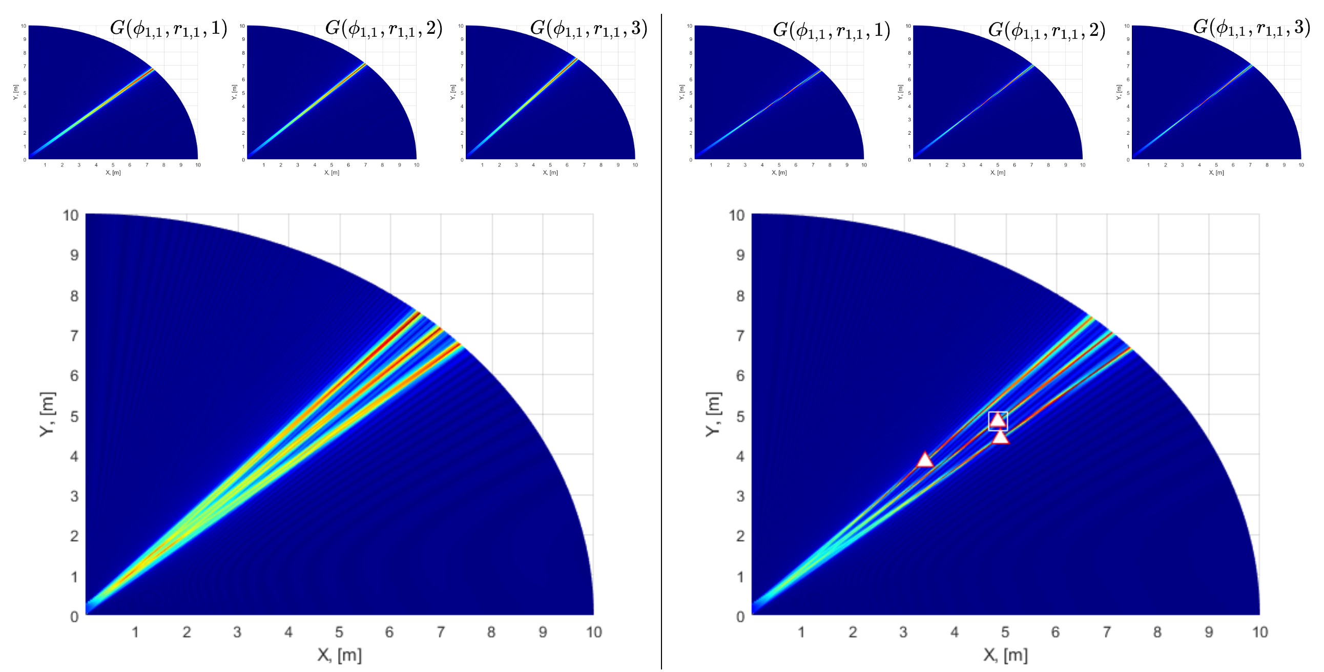
The aforementioned THz works [14, 16, 19, 18, 17, 15] as well as the conventional wireless systems operating at sub-$6$ GHz and mm-Wave bands [10, 11, 12, 13] mostly incorporate far-field plane-wave model whereas the transmission range is shorter in THz-band such that the users are usually in the near-field region [4]. Specifically, the plane wavefront is spherical in the near-field when the transmission range is shorter than the Fraunhofer distance [23]. As a result, the channel acquisition algorithms should take into account near-field model (see, e.g., Fig. 3), which depends on both direction and range information for accurate signal processing [3]. Among the works investigating the near-field signal model, [24, 25, 26, 27, 28] consider the near-field scenario while the effect of beam-split is ignored and only mm-Wave scenario is investigated. In particular, [27] considers the wideband mm-Wave channel estimation while the authors in [28] devise a machine learning (ML)-based approach for narrowband near-field channel estimation. In addition to near-field-only model, hybrid (near- and far-field) models are also present in the literature [24, 26], wherein only narrowband transceiver architectures are considered. On the other hand, several methods have been proposed to compensate the far-field beam-split for both THz channel estimation [16, 19, 14, 15] and beamforming [29, 17, 30] applications. Nevertheless, THz channel estimation in the presence of near-field beam-split (NB) remains relatively unexamined.

In this work, we introduce both a model-based and a model-free techniques for near-field THz channel estimation in the presence of NB. In the model-based approach, we propose an NB-aware (NBA) THz channel estimation technique based on OMP, henceforth called NBA-OMP. For the model-free approach, we devise a federated learning (FL) approach, which is more communication-efficient as compared to conventional centralized learning (CL)-based methods.

We design a novel NBA dictionary, whose columns are composed of near-field subcarrier-dependent (SD) steering vectors spanning the whole angular spectrum and the transmission ranges up to the Fraunhofer distance. Then, we introduce our proposed NBA-OMP approach for wideband THz channel estimation.

The key idea of the proposed approach is that the degree of beam-split is proportionally known prior to the direction-of-arrival (DoA)/range estimation while it depends on the unknown user location. For example, consider $f_{m}$ and $f_{c}$ to be the frequencies for the $m$-th and center subcarriers, respectively. When $\theta$ is the physical user direction, the spatial direction corresponding to the $m$-th-subcarrier is shifted by $\frac{f_{c}}{f_{m}}\theta$. Thus, we employ the OMP algorithm, which accounts for this deviation thereby ipso facto compensating the effect of NB. We have conducted several numerical experiments to demonstrate the effectiveness of the proposed approach in comparison with the existing THz channel-estimation-based methods [24, 15].

Due to limited reflected path components and negligible scattering, the THz channel is usually constructed as the superposition of a single LoS path with a few assisting NLoS paths [4, 29, 9]. In addition, multipath channel models are also widely used, especially for indoor applications [31, 4]. Hence, we consider a general scenario, wherein the $N\times 1$ channel matrix for the $k$-th user at the $m$-th subcarrier is represented by the combination of $L$ paths as [4]

where $\tau_{k,l}$ represents the time delay of the $l$-th path corresponding to the array origin. $\alpha_{k,m,l}\in\mathbb{C}$ denotes the complex path gain and the expected value of its magnitude for the indoor THz multipath model is given by

where $f_{m}$ is the $m$-th subcarrier frequency, $c_{0}$ is speed of light, $r_{k,l}$ represents the distance from the $k$-th user to the array origin and $k_{\mathrm{abs}}(f_{m})$ is the SD medium absorption coefficient [4, 32, 33]. Furthermore, $f_{m}=f_{c}+\frac{B}{M}(m-1-\frac{M-1}{2})$, where $f_{c}$ and $B$ are carrier frequency and bandwidth, respectively.

Due to high frequency operations as well as employing extremely small array aperture, THz-band transmission is likely to encounter near-field phenomenon for close-proximity users. Specifically, the far-field model involves the reception of the transmitted signal at the users as plane-wave. However, the plane wavefront is spherical in the near-field if the transmission range is shorter than the Fraunhofer distance $F=\frac{2D^{2}}{\lambda}$, where $D$ is the array aperture and $\lambda=\frac{c_{0}}{f_{c}}$ is the wavelength [23, 19]. The illustration of beam-split for both far-field and near-field models is given in Fig. 3. For a uniform linear array (ULA), the array aperture is $D=(N-1)d$, where $d=\frac{\lambda}{2}$ is the element spacing. Thus, for THz-band transmission, this distance becomes small such that the near-field signal model should be employed since $r_{k,l}<F$. For instance, when $f_{c}=300$ GHz and $N=256$, the Fraunhofer distance is $F=32.76$ m.

We define the near-field steering vector $\mathbf{a}(\phi_{k,l},r_{k,l})\in\mathbb{C}^{N}$ corresponding to the physical DoA $\phi_{k,l}$ and range $r_{k,l}$ as

where $\phi_{k,l}=\sin\tilde{\phi}_{k,l}$ with $\tilde{\phi}_{k,l}\in[-\frac{\pi}{2},\frac{\pi}{2}]$, and $r_{k,l}^{(n)}$ is the distance between the $k$-th user and the $n$-th antenna as

Following the Fresnel approximation  [34, 23], (6) becomes

where $\zeta_{k,l}=\frac{1-\phi_{k,l}^{2}}{2r_{k,l}}$. Rewrite (5) as

where the $n$-th element of $\tilde{\mathbf{a}}(\phi_{k,l},r_{k,l})\in\mathbb{C}^{N}$ is

The steering vector in (8) corresponds to the physical location $(\phi_{k,l},r_{k,l})$, which deviates to the spatial location $(\bar{\phi}_{k,m,l},\bar{r}_{k,m,l})$ in the beamspace arising from the absent of SD analog beamformers. Then, the $n$-th entry of the deviated steering vector in (9) for the spatial location is

The aim of this work is to estimate the wideband THz channel $\mathbf{h}_{k}[m]$ in the presence of NB in downlink scenario.

Assumption 1: For the proposed model-based technique, we assume that the users are synchronized and they use the received pilot signals transmitted by the BS. We also assume that all users are in the near-field region of the BS, i.e., $r_{k,l}\leq F$.

Assumption 2: For the proposed model-free technique, it is assumed that the datasets of all users are collected prior to the model training stage, and the labels of these datasets are determined by the model-based technique introduced in Sec. IV.

In what follows, we first introduce the NB model, then present the proposed approaches for model-based and model-free channel estimation in the presence of NB.

The key idea of the proposed NBA dictionary design is to utilize the prior knowledge of $\eta_{m}$ to obtain beam-split-corrected steering vectors. In other words, for an arbitrary physical DoA and range, we can readily find the spatial DoA and ranges as $\bar{\phi}=\eta_{m}\phi$ and $\bar{r}=\frac{1-\eta_{m}^{2}\phi^{2}}{\eta_{m}(1-\phi^{2})}r$. Using this observation, we design the NBA dictionary $\mathcal{C}_{m}$ composed of steering vectors $\mathbf{c}(\phi_{m},r_{m})\in\mathbb{C}^{N}$ as

where the $n$-th element of $\mathbf{c}(\phi_{m},r_{m})$ is

where $\zeta_{m}=\frac{1-\phi_{m}^{2}}{2r_{m}}$.

Using the NBA dictionary $\mathcal{C}_{m}$, instead of SI steering vectors $\mathbf{a}(\phi,r)$, the SD virtual steering vectors $\mathbf{c}(\phi_{m},r_{m})$ can be constructed for the OMP algorithm. Once the beamspace spectra is computed via OMP, the sparse channel support corresponding to the SD spatial DoA and ranges are obtained. Then, one can readily find the physical DoAs and ranges as $\phi=\phi_{m}/\eta_{m}$ and ${r}=\frac{\eta_{m}(1-\phi^{2})}{1-\eta_{m}^{2}\phi^{2}}r_{m}$, $\forall m\in\mathcal{M}$.

The proposed NBA dictionary $\mathcal{C}_{m}$ also holds spatial orthogonality as

In the next section, we present the channel estimation procedure with the proposed NBA dictionary.

In downlink, the channel estimation stage is performed simultaneously during channel training by all the users, i.e., $k\in\mathcal{K}=\{1,\cdots,K\}$. Since the BS employs hybrid beamforming architecture, it activates only a single RF chain in each channel use to transmit the pilot signals during channel acquisition [5]. Denote $\tilde{\mathbf{S}}[m]=\mathrm{diag}\{\tilde{s}_{1}[m],\cdots,\tilde{s}_{P}[m]\}$ as the $P\times P$ orthogonal pilot signal matrix, then the BS employs $P$ beamformer vectors as $\tilde{\mathbf{F}}=[\tilde{\mathbf{f}}_{1},\cdots,\tilde{\mathbf{f}}_{P}]\in\mathbb{C}^{N\times P}$ ($|\tilde{\mathbf{f}}_{p}|=1/\sqrt{N}$) to send $P$ orthogonal pilots, which are collected by the $k$-th user as

where $\bar{\mathbf{F}}[m]=\tilde{\mathbf{F}}^{\textsf{T}}[m]\in\mathbb{C}^{P\times N}$. Assume that $\bar{\mathbf{F}}[m]=\mathbf{F}\in\mathbb{C}^{P\times N}$ and $\tilde{\mathbf{S}}[m]=\mathbf{I}_{P},\forall m\in\mathcal{M}$ [10, 14, 15], we get

Note that the solution via traditional techniques, e.g., the least squares (LS) and MMSE estimator can be readily given respectively as

where $\mathbf{R}_{k}[m]=\mathbb{E}\{\mathbf{h}_{k}[m]\mathbf{h}_{k}^{\textsf{H}}[m]\}$ is the channel covariance matrix. Nevertheless, these methods require either prior information (e.g., MMSE) or have poor estimation performance (e.g., LS) [35, 13]. Furthermore, these methods require at least $P\geq N$ pilot signals, which can be heavy for channel training while our proposed approach exhibits a much lower channel training overhead (e.g, see Sec. VI).

By exploiting the THz channel sparsity, the THz channel can be represented in a sparse domain via support vector $\mathbf{x}_{k}[m]\in\mathbb{C}^{Q}$, which is an $L$-sparse vector, whose non-zero elements corresponds to the set

Then, the received signal in (24) is rewritten in sparse domain as

where $\mathbf{F}$ is an $P\times N$ fixed matrix corresponding to the hybrid beamformer weights during data transmission, and $\mathbf{C}_{m}$ is the ${N\times Q}$ NBA dictionary matrix covering the spatial domain with $\phi_{m,q}\in[-\eta_{m},\eta_{m}]$ ($\phi\in[-1,1]$) and $r_{m,q}\in[0,F]$ for $q=1,\cdots,Q$ as

By utilizing the NBA dictionary matrix $\mathbf{C}_{m}$, we employ the OMP algorithm to effectively recover the sparse channel support. The proposed NBA-OMP technique is presented in Algorithm 1, which accepts $\mathbf{y}_{k}[m]$, $\mathbf{C}_{m}$ and $\eta_{m}$ as inputs and it yields the output as the estimated channel $\hat{\mathbf{h}}_{k}[m]$, and the near-field beam-split in terms of DoA and ranges, i.e., $\hat{\Delta}(\phi_{k,l},m)$ and $\hat{\Delta}(r_{k,l},m)$, respectively. In steps $4-6$ of Algorithm 1, the orthogonality between the residual observation vector $\mathbf{r}_{l}[m]$ and the columns of the dictionary matrix is checked as

where $q^{\star}$ denotes the support index for the $l$th path iteration. Then, the DoA and range estimates can be found as $\hat{\phi}_{k,l}=\frac{\phi_{m,q^{\star}}}{\eta_{m}}$ and $\hat{r}_{k,l}=\frac{\eta_{m}(1-\phi_{m,q^{\star}}^{2})}{1-\eta_{m}^{2}\phi_{m,q^{\star}}}r_{m,q^{\star}}$, respectively. In a similar way, the corresponding beam-split terms are $\hat{\Delta}(\phi_{k,l},m)=(\eta_{m}-1)\hat{\phi}_{k,l}$ and $\hat{\Delta}(r_{k,l},m)\hskip-3.0pt=\hskip-2.0pt(\eta_{m}\hskip-2.0pt-\hskip-2.0pt1)\frac{1-\eta_{m}^{2}\hat{\phi}_{k,l}^{2}}{\eta_{m}(1-\hat{\phi}_{k,l}^{2})}\hat{r}_{k,l}$. Once the DoA and ranges are obtained, the THz channel is constructed from the estimated support as $\hat{\mathbf{h}}_{k}[m]=\boldsymbol{\Xi}_{k}\hat{\mathbf{u}}_{k}[m]$ where $\boldsymbol{\Xi}_{k}=[\mathbf{a}(\hat{\phi}_{k,1},\hat{r}_{k,1}),\cdots,\mathbf{a}(\hat{\phi}_{k,L},\hat{r}_{k,L})]$ and $\hat{\mathbf{u}}_{k}[m]=\boldsymbol{\Psi}_{m}^{\dagger}(\mathcal{I}_{L})\mathbf{y}_{k}[m]$, wherein $\boldsymbol{\Psi}_{m}(\mathcal{I}_{L})=\mathbf{F}\mathbf{C}_{m}(\mathcal{I}_{L})$ and $\mathcal{I}_{L}$ includes the estimated support indices.

The computational complexity of NBA-OMP is the same as traditional OMP techniques [5], and it is mainly due to the matrix multiplications in step $4$ $(O(QMNP(NP+P)))$, step $10$ $(O(PNL\bar{L}))$, step $11$ $(O(P^{2}L\bar{L}+P^{2}))$ and step $16$ $(O(L(P+N)))$, where $\bar{L}=(L+1)/2$. Hence, the overall complexity is $O(QMNP(NP+P)+(PL\bar{L}+1)(N+P))$.

The channel training overhead of the NBA-OMP requires only $P$ ($8$ times lower, see Sec. VII) channel usage for pilot signaling while the traditional approaches, e.g., LS and MMSE estimation, need at least $N$ channel usage.

The communication overhead of a learning-based approach can be measured in terms of amount of data symbols transmitted during/for model training [35, 16, 37, 38, 39]. Thus, the communication overhead (i.e., $\mathcal{T}_{\mathrm{CL}}$) for the CL involves the amount of dataset transmitted from the users to the server whereas it can be computed for FL (i.e., $\mathcal{T}_{\mathrm{FL}}$) as the amount of model parameters exchanged between the users and the server during training. Then, we have

where $\textsf{D}_{k}$ is the number of samples of the $k$-th dataset and $3N_{\mathrm{RF}}+2N$ is the number of symbols in each input-output (i.e., $\mathcal{X}_{k}^{(i)}-\mathcal{Y}_{k}^{(i)}$) tuple. In (37), $\xi$ denotes whether the labels are also transmitted from the users to the server. Thus, if the labels are computed at the users, they are transmitted to the server with additional overhead, and we have $\xi=1$. On the other hand, $\xi=0$ (labels are not computed at the user) if the received inputs are transmitted to the server, at which the labeling (channel estimation) is handled, thereby less communication overhead is achieved. Next, we defined the communication overhead for FL as

which involves a two-way (user $\rightleftarrows$ server) transmission of the learnable parameters from $K$ users to the server for $T$ consecutive iterations.

References

- [1] T. S. Rappaport, Y. Xing, O. Kanhere, S. Ju, A. Madanayake, S. Mandal, A. Alkhateeb, and G. C. Trichopoulos, “Wireless communications and applications above 100 GHz: Opportunities and challenges for 6G and beyond,” IEEE Access, vol. 7, pp. 78 729–78 757, Jun. 2019.
- [2] I. F. Akyildiz, C. Han, Z. Hu, S. Nie, and J. M. Jornet, “Terahertz Band Communication: An Old Problem Revisited and Research Directions for the Next Decade,” IEEE Trans. Commun., vol. 70, no. 6, pp. 4250–4285, May 2022.
- [3] A. M. Elbir, K. V. Mishra, S. Chatzinotas, and M. Bennis, “Terahertz-band integrated sensing and communications: Challenges and opportunities,” arXiv preprint arXiv:2208.01235, Aug. 2022.
- [4] H. Sarieddeen, M.-S. Alouini, and T. Y. Al-Naffouri, “An overview of signal processing techniques for terahertz communications,” Proceedings of the IEEE, vol. 109, no. 10, pp. 1628–1665, 2021.
- [5] R. W. Heath, N. González-Prelcic, S. Rangan, W. Roh, and A. M. Sayeed, “An overview of signal processing techniques for millimeter wave MIMO systems,” IEEE J. Sel. Top. Signal Process., vol. 10, no. 3, pp. 436–453, Feb. 2016.
- [6] A. M. Elbir, K. V. Mishra, S. A. Vorobyov, and W. Heath Robert, Jr., “Twenty-five years of advances in beamforming: From convex and nonconvex optimization to learning techniques,” arXiv preprint arXiv:2211.02165, Nov. 2022.
- [7] A. Alkhateeb and R. W. Heath, “Frequency selective hybrid precoding for limited feedback millimeter wave systems,” IEEE Trans. Commun., vol. 64, no. 5, pp. 1801–1818, 2016.
- [8] X. Yu, J. Shen, J. Zhang, and K. B. Letaief, “Alternating minimization algorithms for hybrid precoding in millimeter wave MIMO systems,” IEEE J. Sel. Topics Signal Process., vol. 10, no. 3, pp. 485–500, April 2016.
- [9] J. Tan and L. Dai, “Wideband beam tracking in THz massive MIMO systems,” IEEE J. Sel. Areas Commun., vol. 39, no. 6, pp. 1693–1710, Apr 2021.
- [10] A. Alkhateeb, G. Leus, and R. W. Heath, “Limited feedback hybrid precoding for multi-user millimeter wave systems,” IEEE Trans. Wireless Commun., vol. 14, no. 11, pp. 6481–6494, Jul. 2015.
- [11] H. Yin, D. Gesbert, M. Filippou, and Y. Liu, “A Coordinated Approach to Channel Estimation in Large-Scale Multiple-Antenna Systems,” IEEE J. Sel. Areas Commun., vol. 31, no. 2, pp. 264–273, February 2013.
- [12] Z. Marzi, D. Ramasamy, and U. Madhow, “Compressive Channel Estimation and Tracking for Large Arrays in mm-Wave Picocells,” IEEE J. Sel. Topics Signal Process., vol. 10, no. 3, pp. 514–527, April 2016.
- [13] J. Wang, Z. Lan, C. woo Pyo, T. Baykas, C. sean Sum, M. A. Rahman, J. Gao, R. Funada, F. Kojima, H. Harada, and S. Kato, “Beam codebook based beamforming protocol for multi-Gbps millimeter-wave WPAN systems,” IEEE J. Sel. Areas Commun., vol. 27, no. 8, pp. 1390–1399, October 2009.
- [14] K. Dovelos, M. Matthaiou, H. Q. Ngo, and B. Bellalta, “Channel estimation and hybrid combining for wideband terahertz massive MIMO systems,” IEEE J. Sel. Areas Commun., vol. 39, no. 6, pp. 1604–1620, Apr. 2021.
- [15] J. Tan and L. Dai, “Wideband channel estimation for THz massive MIMO,” China Commun., vol. 18, no. 5, pp. 66–80, May 2021.
- [16] A. M. Elbir, W. Shi, K. V. Mishra, and S. Chatzinotas, “Federated Multi-Task Learning for THz Wideband Channel and DoA Estimation,” arXiv preprint arXiv:2207.06017, Jul. 2022.
- [17] A. M. Elbir, “A Unified Approach for Beam-Split Mitigation in Terahertz Wideband Hybrid Beamforming,” arXiv preprint arXiv:2209.12097, Sep. 2022.
- [18] B. Wang, F. Gao, S. Jin, H. Lin, and G. Y. Li, “Spatial- and Frequency-Wideband Effects in Millimeter-Wave Massive MIMO Systems,” IEEE Trans. Signal Process., vol. 66, no. 13, pp. 3393–3406, May 2018.
- [19] A. M. Elbir, W. Shi, A. K. Papazafeiropoulos, P. Kourtessis, and S. Chatzinotas, “Terahertz-band channel and beam split estimation via array perturbation model,” arXiv preprint arXiv:2208.03683, Aug. 2022.
- [20] S. Nie and I. F. Akyildiz, “Deep Kernel Learning-Based Channel Estimation in Ultra-Massive MIMO Communications at 0.06-10 THz,” in 2019 IEEE Globecom Workshops (GC Wkshps). IEEE, Dec. 2019, pp. 1–6.
- [21] Y. Chen and C. Han, “Deep CNN-Based Spherical-Wave Channel Estimation for Terahertz Ultra-Massive MIMO Systems,” in GLOBECOM 2020 - 2020 IEEE Global Communications Conference. IEEE, Dec. 2020, pp. 1–6.
- [22] E. Balevi and J. G. Andrews, “Wideband Channel Estimation With a Generative Adversarial Network,” IEEE Trans. Wireless Commun., vol. 20, no. 5, pp. 3049–3060, Jan. 2021.
- [23] E. Björnson, Ö. T. Demir, and L. Sanguinetti, “A Primer on Near-Field Beamforming for Arrays and Reconfigurable Intelligent Surfaces,” arXiv preprint arXiv:2110.06661, Oct. 2021.
- [24] X. Wei and L. Dai, “Channel Estimation for Extremely Large-Scale Massive MIMO: Far-Field, Near-Field, or Hybrid-Field?” IEEE Commun. Lett., vol. 26, no. 1, pp. 177–181, Nov. 2021.
- [25] M. Cui and L. Dai, “Channel Estimation for Extremely Large-Scale MIMO: Far-Field or Near-Field?” IEEE Trans. Commun., vol. 70, no. 4, pp. 2663–2677, Jan. 2022.
- [26] W. Yu, Y. Shen, H. He, X. Yu, J. Zhang, and K. B. Letaief, “Hybrid Far- and Near-Field Channel Estimation for THz Ultra-Massive MIMO via Fixed Point Networks,” arXiv preprint arXiv:2205.04944, May 2022.
- [27] X. Zhang, H. Zhang, and Y. C. Eldar, “Near-Field Sparse Channel Representation and Estimation in 6G Wireless Communications,” arXiv preprint arXiv:2212.13527, Dec. 2022.
- [28] X. Zhang, Z. Wang, H. Zhang, and L. Yang, “Near-Field Channel Estimation for Extremely Large-Scale Array Communications: A model-based deep learning approach,” arXiv preprint arXiv:2211.15440, Nov. 2022.
- [29] A. M. Elbir, K. V. Mishra, and S. Chatzinotas, “Terahertz-band joint ultra-massive MIMO radar-communications: Model-based and model-free hybrid beamforming,” IEEE J. Sel. Top. Signal Process., vol. 15, no. 6, pp. 1468–1483, Oct. 2021.
- [30] L. Dai, J. Tan, Z. Chen, and H. V. Poor, “Delay-phase precoding for wideband THz massive MIMO,” IEEE Trans. Wireless Commun., p. 1, Mar. 2022.
- [31] S. Tarboush, H. Sarieddeen, H. Chen, M. H. Loukil, H. Jemaa, M. S. Alouini, and T. Y. Al-Naffouri, “TeraMIMO: A channel simulator for wideband ultra-massive MIMO terahertz communications,” arXiv, Apr 2021.
- [32] H. Yuan, N. Yang, K. Yang, C. Han, and J. An, “Hybrid beamforming for terahertz multi-carrier systems over frequency selective fading,” IEEE Trans. Commun., vol. 68, no. 10, pp. 6186–6199, Jul 2020.
- [33] H. Yuan, N. Yang, X. Ding, C. Han, K. Yang, and J. An, “Cluster-based multi-carrier hybrid beamforming for massive device terahertz communications,” IEEE Trans. Commun., vol. 70, no. 5, pp. 3407–3420, Mar. 2022.
- [34] M. Cui, L. Dai, Z. Wang, S. Zhou, and N. Ge, “Near-Field Rainbow: Wideband Beam Training for XL-MIMO,” IEEE Trans. Wireless Commun., p. 1, Nov. 2022.
- [35] A. M. Elbir and S. Coleri, “Federated Learning for Channel Estimation in Conventional and RIS-Assisted Massive MIMO,” IEEE Trans. Wireless Commun., vol. 21, no. 6, pp. 4255–4268, Nov. 2021.
- [36] A. M. Elbir, A. K. Papazafeiropoulos, and S. Chatzinotas, “Federated Learning for Physical Layer Design,” IEEE Commun. Mag., vol. 59, no. 11, pp. 81–87, Nov. 2021.
- [37] H. B. McMahan, E. Moore, D. Ramage, S. Hampson, and B. A. y. Arcas, “Communication-Efficient Learning of Deep Networks from Decentralized Data,” arXiv, Feb 2016.
- [38] M. M. Amiri and D. Gündüz, “Federated Learning Over Wireless Fading Channels,” IEEE Trans. Wireless Commun., vol. 19, no. 5, pp. 3546–3557, 2020.
- [39] M. Mohammadi Amiri and D. Gündüz, “Machine learning at the wireless edge: Distributed stochastic gradient descent over-the-air,” IEEE Trans. Signal Process., vol. 68, pp. 2155–2169, 2020.
- [40] J. Rodríguez-Fernández, N. González-Prelcic, K. Venugopal, and R. W. Heath, “Frequency-Domain Compressive Channel Estimation for Frequency-Selective Hybrid Millimeter Wave MIMO Systems,” IEEE Trans. Wireless Commun., vol. 17, no. 5, pp. 2946–2960, Mar. 2018.