Fuzzing Automatic Differentiation in Deep-Learning Libraries

Chenyuan Yang Affiliation: University of Illinois
Urbana-Champaign
cy54@illinois.edu Yuxing Tu Affiliation: Huazhong University of
Science and Technology
yxtu@hust.edu.cn Yinlin Deng Affiliation: University of Illinois
Urbana-Champaign
yinlind2@illinois.edu Hanchi Li Affiliation: University of Science
and Technology of China
slxiaochi@mail.ustc.edu.cn Jiayi Yao Affiliation: The Chinese University of
Hong Kong, Shenzhen
jiayiyao@link.cuhk.edu.cn Lingming Zhang Affiliation: University of Illinois
Urbana-Champaign
lingming@illinois.edu

Abstract

Deep learning (DL) has attracted wide attention and has been widely deployed in recent years. As a result, more and more research efforts have been dedicated to testing DL libraries and frameworks. However, existing work largely overlooked one crucial component of any DL system, automatic differentiation (AD), which is the basis for the recent development of DL. To this end, we propose $\nabla$ Fuzz, the first general and practical approach specifically targeting the critical AD component in DL libraries. Our key insight is that each DL library API can be abstracted into a function processing tensors/vectors, which can be differentially tested under various execution scenarios (for computing outputs/gradients with different implementations). We have implemented $\nabla$ Fuzz as a fully automated API-level fuzzer targeting AD in DL libraries, which utilizes differential testing on different execution scenarios to test both first-order and high-order gradients, and also includes automated filtering strategies to remove false positives caused by numerical instability. We have performed an extensive study on four of the most popular and actively-maintained DL libraries, PyTorch, TensorFlow, JAX, and OneFlow. The result shows that $\nabla$ Fuzz substantially outperforms state-of-the-art fuzzers in terms of both code coverage and bug detection. To date, $\nabla$ Fuzz has detected 173 bugs for the studied DL libraries, with 144 already confirmed by developers (117 of which are previously unknown bugs and 107 are related to AD). Remarkably, $\nabla$ Fuzz contributed 58.3% (7/12) of all high-priority AD bugs for PyTorch and JAX during a two-month period.None of the confirmed AD bugs were detected by existing fuzzers.

I Introduction

Recent years have witnessed the rapid advancement of deep learning (DL) research and the wide adoption of DL solutions/technologies in various application domains, e.g., natural language processing [1], healthcare [2], scientific discovery [3], and software engineering [4, 5, 6, 7, 8, 9]. As a result, there is a growing concern about the correctness and reliability of such systems. For example, for a safety-critical application domain such as autonomous driving, a bug in the DL system can cause serious consequences or even death [10].

As it is critical to ensure the quality of increasingly influential DL systems, much research attention has been focused on testing/verifying DL models [11, 12, 13, 14, 15, 16, 17, 18, 19, 20, 21] or application programs [22, 23, 24]. Recently, testing underlying DL libraries/frameworks (e.g., PyTorch/TensorFlow) has also drawn wide attention, since DL libraries serve as the central infrastructure for all DL applications.CRADLE [25] is one of the pioneering work to perform differential testing on multiple backends of Keras [26] using various DL models. AUDEE [27] and LEMON [28] further apply search-based mutation strategies on existing models to generate more diverse test inputs. While these mutation-based techniques heavily rely on seed models, Muffin [29] directly synthesizes DL models from DL APIs via a top-down generation approach. Moreover, Muffin can detect inconsistencies in both the model training and inference phases across different backends of Keras. Unlike the above model-level testing techniques, the recent FreeFuzz work [30] proposes a fully-automated API-level fuzzing technique via mining API inputs from open source. Similarly, another recent work, DocTer [31], directly generates inputs for each API based on DL-specific input constraints extracted from DL API documentation (assisted with human annotations). Despite the recent advances in DL library testing, existing techniques still suffer from a major limitation: The inference phase of DL models or the direct execution of DL APIs has received the most attention, while a crucial component of any DL system - automatic differentiation (AD) [32] - is still understudied. Many DL algorithms, notably back-propagation [33], one of the key algorithms for training feed-forward neural networks, rely heavily on AD for derivative computation of arbitrary numerical functions.AD enables the development of sophisticated DL models and algorithms since, without AD, people would have to manually/symbolically calculate the derivatives of billions of parameters for large DL models [34]. To obtain the derivatives automatically, special gradient/Jacobian computation operations in DL libraries need to be explicitly triggered (e.g., tf.GradientTape.gradient() in TensorFlow).Notably, bugs in AD may cause DL models to fail to converge and/or perform poorly in practical deployment, which is fatal for safety-critical applications. For example, silent AD computation bugs may cause the output of the deployed DL models to diverge significantly from the output in the training phase. Besides, AD bugs may also directly crash the entire training process, wasting massive computation resources when training recent popular large models and/or causing potential denial-of-service (DoS) attacks [35]. Figure 1 shows a dangerous crash bug where a widely used PyTorch API KLDivLoss [36] will crash during AD computation with a special input shape.However, such AD engines have not been thoroughly tested by existing work.

Fig. 1: Crash bug in AD

Although the recent Muffin work [29] can potentially test the training phase of DL models, it is still far from practical. First, Muffin needs to manually annotate the input constraints of considered DL APIs and use reshaping operations to ensure the validity of the generated models.As a result, Muffin can only cover a small set of APIs (confirmed in §VI-A). Second, whole model testing is inefficient, especially for large models/datasets.Third, false positives can originate from randomness, precision loss, and numerical instability, which are further amplified in the model training scenario.Fourth, differential testing of the training phase requires the same API interfaces across different DL libraries, which further limits its application. Muffin uses Keras and its supported backends TensorFlow, Theano, and CNTK. However, Keras 2.3.0 in 2019 is the last release supporting backends other than TensorFlow [37].Lastly, Muffin cannot fully test the AD engines in DL libraries, as it only covers part of reverse mode AD and ignores forward mode AD. In fact, the Muffin paper did not report any confirmed AD bug (confirmed in §VI-A).

To thoroughly and automatically test the AD engines in DL libraries, we propose $\nabla$ Fuzz, the first general and practical framework specifically targeting the crucial AD component. Our key insight is that each API in a DL library can be abstracted into a function processing tensors/vectors, which can be differentially tested under various execution scenarios (for computing outputs/gradients with different implementations). For example, the same DL API can be executed without AD or with different AD modes, but both the API output and gradient should be consistent across different execution scenarios, which can naturally serve as the oracle for differential testing. In addition, since our test oracle is general at the function level, we can further transform each API into its gradient function to test the correctness of high-order gradient computation.

$\nabla$ Fuzz can potentially address all the aforementioned limitations of Muffin. Through API-level testing, $\nabla$ Fuzz no longer suffers from strict input constraints in model-level testing, and can be fully automated. Also, API-level mutation is more efficient because it avoids extensive computation on large models with large datasets. Besides, false positives can be significantly reduced, since floating-point precision loss will not be accumulated in API-level testing.Lastly, compared to Muffin, our technique is also more general, because we utilize the natural AD oracles available in any DL library.

We have implemented $\nabla$ Fuzz as a fully automated technique for API-level fuzzing with test oracles specifically targeting AD in DL libraries. More precisely, while our approach is general and can leverage any existing API-level DL library fuzzer for input generation, we build $\nabla$ Fuzz on top of state-of-the-art FreeFuzz [38] because it is fully automated and publicly available. For test oracle, $\nabla$ Fuzz automatically performs differential testing of each DL library API (and its high-order gradients) under different execution scenarios provided by the underlying DL library. $\nabla$ Fuzz also incorporates automated filter strategies to further reduce false positives caused by numerical instability issues. We have conducted an extensive study of $\nabla$ Fuzz on four of the most widely-used and actively-maintained DL libraries: PyTorch, TensorFlow, JAX, and OneFlow. Our results show that $\nabla$ Fuzz substantially outperforms state-of-the-art DL library fuzzers (including both FreeFuzz and Muffin) in terms of both code coverage and bug detection. In fact, the bug in Figure 1 is detected by $\nabla$ Fuzz and cannot be detected by any previous techniques.Overall, our paper makes the following contributions:

1.

To the best of our knowledge, this is the first work specifically targeting fuzzing the crucial AD component in DL libraries with practical and general test oracles. Our proposed AD oracles can potentially strengthen and impact all future work on fuzzing DL libraries/systems.
2.

We have implemented $\nabla$ Fuzz as a fully automated technique for testing AD in DL libraries. $\nabla$ Fuzz is built on state-of-the-art FreeFuzz and resolves the test oracle challenge with differential testing on various differentiation scenarios; $\nabla$ Fuzz can also test the correctness of gradient computation of any order. Moreover, we have also designed novel strategies to filter out false positives.
3.

We conduct an extensive study on popular DL libraries (PyTorch, TensorFlow, JAX, and OneFlow). $\nabla$ Fuzz has detected 173 bugs in total, with 144 confirmed by developers (117 are previously unknown and 107 are AD-related) and 38 already fixed. Remarkably, $\nabla$ Fuzz contributed 58.3% (7/12) of all high-priority AD bugs for PyTorch and JAX within two months. None of the 107 AD-related bugs can be detected by existing work.

II Background

II-A Basics about DL Libraries

Refer to caption — Fig. 2: An example of DL model training and inference

DL Models and DL APIs. To develop a DL pipeline, users usually call DL APIs in a DL program to accomplish the following: build a DL model, load a dataset, train the DL model with labeled training data, and test it with evaluation data. The example TensorFlow program shown in the left side of Figure 2 constructs a dense neural network, which contains two Dense layers, with relu and softmax as the activation functions. Starting from an input layer input, the tensor output is obtained by invoking the DL APIs sequentially. The model is then constructed by defining the inputs and outputs, and compiled with specified optimizer (SGD) and loss function (MeanAbsoluteError). Next, we train the model with the high-level API model.fit and make predictions with model.predict.

Training phase. For model training, DL libraries usually provide high-level APIs (e.g., model.fit() in TensorFlow) for ease of use. However, the actual training phase is complicated and composed of three stages: forward pass, loss computation, and backward pass. Such training steps will be carried out repeatedly until convergence. Figure 2 depicts an illustration of one training step for the example program, where W1 and W2 stand for the weight tensors of Dense layers. During the forward pass when the output tensor is computed with input and weight tensors, every executed operation will be automatically recorded for automatic differentiation (AD). Please note that additional traced information is omitted in Figure 2 for simplicity. After loss computation (requiring labels), the recorded AD context will be used to compute gradients (Grad1, Grad2) of the loss w.r.t the weight tensors. Lastly, the optimizer will apply the gradients to update W1 and W2 by adding $\Delta$ W1 and $\Delta$ W2 (computed from the gradients).

Inference phase. During the inference phase, DL APIs will be executed to compute the output tensor as in the forward pass, except that AD is usually disabled for efficiency.

II-B Automatic Differentiation

Automatic differentiation (AD) is one of the core components of DL frameworks, which contributes substantially to the success of DL. AD decomposes a function/model into a set of elementary operations for which derivatives are known and leverages chain rule to compose the derivatives of these operations [39]. It allows us to calculate the derivative of any function/model without extensive manual effort. AD usually has two distinct modes, reverse mode (or reverse accumulation) and forward mode (or forward accumulation).

Reverse Mode. Reverse mode is the most common AD mode in DL libraries. It evaluates the chain rule from the output to the input, which is the reverse order of the original function/model. Reverse mode calculates the derivative in two different phases: forward phase and backward phase. In the forward phase, we will obtain the output of the original function, and evaluate the output value and all the intermediate variables, whose values are stored in memory. In the backward phase, derivatives are calculated by leveraging the chain rule and the intermediate value, which could propagate back the derivative from the output to the input.

Figure 3 presents an example function $f(x_{1},x_{2})$ together with its computation graph.When $(x_{1},x_{2})$ is $(1,2)$ , the trace of computation of reverse mode AD is shown in Table I. To simplify the representations, we use $\bar{v}=\frac{\partial f}{\partial v}$ to represent the partial derivative of $f$ w.r.t the variant $v$ . First, the function evaluates the output value ( $f=1.53$ ) and stores all the intermediate values in the forward phase, shown on the left side of Table I. Because the derivatives of the elementary operations are known, e.g., the derivative of $\sin(x_{1})$ is $\cos(x_{1})$ , the reverse mode AD can leverage the chain rule and stored values to propagate back the derivative from $f$ to inputs $x_{1},x_{2}$ automatically, shown on the right side of Table I.

It is worth noting that derivatives $\bar{x_{1}}=1.54$ and $\bar{x_{2}}=0.5$ are calculated in just one reverse pass since the output value of this function is scalar. If the function is more general (e.g., $\mathbf{f}:\mathbb{R}^{n}\rightarrow\mathbb{R}^{m}$ ), the reverse mode AD needs $m$ reverse pass to calculate the gradients. As DL usually computes the gradient of a low dimensional tensor (e.g., scalar loss values) w.r.t a huge number of parameters in practice, reverse mode is the main AD used in DL libraries.

TABLE I: Reverse mode AD computation trace

Forward Phase	Backward Phase
$x_{1}=1$	$\bar{x}_{1}=1.54$
$x_{2}=2$	$\bar{x}_{2}=0.5$
$v_{1}=x_{1}\cdot x_{2}=2$	$\bar{x}_{1}=\bar{x}_{1}+\bar{v}_{1}\cdot\frac{\partial v_{1}}{\partial x_{1}}=0.54+0.5\cdot 2=1.54$
	$\bar{x}_{2}=\bar{v}_{1}\cdot\frac{\partial v_{1}}{\partial x_{2}}=0.5$
$v_{2}=\log(v_{1})=0.69$	$\bar{v}_{1}=\bar{v}_{2}\cdot\frac{\partial v_{2}}{\partial v_{1}}=1/v_{1}=0.5$
$v_{3}=\sin(x_{1})=0.84$	$\bar{x}_{1}=\bar{v}_{3}\cdot\frac{\partial v_{3}}{\partial x_{1}}=\cos(1)=0.54$
$v_{4}=v_{2}+v_{3}=1.53$	$\bar{v}_{2}=\bar{v}_{4}\cdot\frac{\partial v_{4}}{\partial v_{2}}=1$
	$\bar{v}_{3}=\bar{v}_{4}\cdot\frac{\partial v_{4}}{\partial v_{3}}=1$
$f=v_{4}=1.53$	$\bar{v}_{4}=\bar{f}=\partial f/\partial v_{4}=1$

Forward Mode. Different from reverse mode, forward mode AD computes the derivatives simultaneously with the original function/model outputs, i.e., it evaluates the chain rule from input to output. Thus, it does not need to store the intermediate values like reverse mode. Forward mode AD also has two phases: forward primal phase and forward tangent phase. The forward primal phase obtains the output of the original function, while concurrently the forward tangent phase calculates the gradient by applying the chain rule from input to output.

Back to $f$ shown in Figure 3, whose forward mode computational trace is shown in Table II. The forward mode AD computes the derivative by applying the chain rule to each elementary operation along the forward primal phase. However, it can only compute the gradient of one input in one pass. In this example, we calculate the partial gradient of $f$ w.r.t $x_{1}$ . For simplicity, we define $\dot{v}=\frac{\partial v}{\partial x_{1}}$ as the partial gradient of $v$ w.r.t to the input $x_{1}$ . Thus, we set $\dot{x_{1}}=1,\dot{x_{2}}=0$ at the beginning since the gradient of $x_{1}$ w.r.t itself is 1 and $x_{2}$ does not affect $x_{1}$ . Along the forward tangent phase shown on the right side of Table II, the final partial gradient $\dot{f}=\frac{\partial f}{\partial x_{1}}$ is 1.54, the same as computed by reverse mode.

In general, for function $\mathbf{f}:\mathbb{R}^{n}\rightarrow\mathbb{R}^{m}$ , forward mode AD requires $n$ evaluations to calculate the gradient by setting $\dot{x_{i}}=1$ and the rest to zero for each input. Thus, forward mode AD can be more time and memory efficient than reverse mode when $n\leq m$ , and is useful in cases like computing the Hessian matrix [40] efficiently.

TABLE II: Forward mode AD computation trace

Forward Primal Phase	Forward Tangent Phase
$x_{1}=1$	$\dot{x}_{1}=1$
$x_{2}=2$	$\dot{x}_{2}=0$
$v_{1}=x_{1}\cdot x_{2}=2$	$\dot{v}_{1}=\dot{x}_{1}\cdot x_{2}=2$
$v_{2}=\log(v_{1})=0.69$	$\dot{v}_{2}=\dot{v}_{1}/v_{1}=1$
$v_{3}=\sin(x_{1})=0.84$	$\dot{v}_{3}=\dot{x_{1}}\cdot\cos(x_{1})=0.54$
$v_{4}=v_{2}+v_{3}=1.53$	$\dot{v}_{4}=\dot{v}_{2}+\dot{v}_{3}=1.54$
$f=v_{4}=1.53$	$\dot{f}=\dot{v}_{4}=1.54$

Despite the recent advances in DL library testing [30, 29, 28, 25, 27, 41, 31], there is still limited work that can effectively test the crucial AD component for DL libraries. Therefore, this paper aims to build the first practical fuzzing technique specifically targeting AD in DL libraries.

III Preliminaries

In this section, we will present the preliminaries for differentiation computations, which are essential for understanding AD implementation in DL libraries and our approach.

III-A Mathematics behind Automatic Differentiation

Differentiation is a process of computing the gradient for a given function at a given point. Especially, the gradient is defined for scalar-valued functions as below:

Definition 1.

Gradient. For a scalar-valued function $f:\mathbb{R}^{n}\rightarrow\mathbb{R}$ and a point $\boldsymbol{x}$ , its gradient at $\boldsymbol{x}$ is defined as below:

\nabla f(\boldsymbol{x})=\begin{bmatrix}\frac{\partial f}{\partial x_{1}}&\cdots&\frac{\partial f}{\partial x_{n}}\end{bmatrix}^{T}

(1)

The gradient can be further generalized to functions that return non-scalar values, namely the Jacobian matrix [42]:

Definition 2.

Jacobian. The Jacobian matrix of a vector-valued function $\mathbf{f}:\mathbb{R}^{n}\rightarrow\mathbb{R}^{m}$ is defined as an $m\times n$ matrix:

\mathbf{J}(\mathbf{f})=\begin{bmatrix}\nabla^{T}f_{1}\\ \vdots\\ \nabla^{T}f_{m}\end{bmatrix}=\begin{bmatrix}\frac{\partial f_{1}}{\partial x_{1}}&\cdots&\frac{\partial f_{1}}{\partial x_{n}}\\ \vdots&\ddots&\vdots\\ \frac{\partial f_{m}}{\partial x_{1}}&\cdots&\frac{\partial f_{m}}{\partial x_{n}}\end{bmatrix}

(2)

where $\mathbf{f}(\boldsymbol{x})=(f_{1}(\boldsymbol{x}),f_{2}(\boldsymbol{x}),\dots,f_{m}(\boldsymbol{x}))$ .

In this paper, for simplicity, we use “gradient” to represent the Jacobian matrix for the vector-valued function. The gradient function of $\mathbf{f}$ is defined as $\mathbf{f}^{\prime}:\mathbb{R}^{n}\rightarrow\mathbb{R}^{m}\times\mathbb{R}^{n}$ , where $\mathbf{f}^{\prime}(\boldsymbol{x})$ is the Jacobian matrix of $\mathbf{f}$ at the point $\boldsymbol{x}$ .

The gradient $\mathbf{f}^{\prime}(\boldsymbol{x})\in\mathbb{R}^{m}\times\mathbb{R}^{n}$ can also be considered as a linear map, which maps the tangent space [43] of the domain of $\mathbf{f}$ at the point $\boldsymbol{x}$ to the tangent space of the codomain of $\mathbf{f}$ at the point $\mathbf{f}(\boldsymbol{x})$ . Given this mapping of $\mathbf{f}^{\prime}(\boldsymbol{x}):\mathbb{R}^{n}\rightarrow\mathbb{R}^{m}$ , we can now define Jacobian-vector product (JVP) and vector-Jacobian product (VJP), which have been adopted as the theoretical basis for efficient DL training and implemented using forward-/reverse-mode AD in DL libraries:

Definition 3.

Jacobian-vector product. Given an input point $\boldsymbol{x}\in\mathbb{R}^{n}$ and a tangent vector $\mathbf{u}\in\mathbb{R}^{n}$ from the tangent space of $\mathbf{f}$ at $\boldsymbol{x}$ , the Jacobian-vector product is defined as below:

\mathrm{JVP}(\boldsymbol{x},\mathbf{u})=\mathbf{f}^{\prime}(\boldsymbol{x})\cdot\mathbf{u}

(3)

JVP computes the directional gradient, with direction $\mathbf{u}\in\mathbb{R}^{n}$ , for the function $\mathbf{f}:\mathbb{R}^{n}\rightarrow\mathbb{R}^{m}$ at the point $\boldsymbol{x}\in\mathbb{R}^{n}$ , and is implemented with forward mode AD in DL libraries. Back to the example shown in Figure 3, the $(\dot{x}_{1},\dot{x}_{2})$ in the forward mode AD trace (Table II) is the tangent vector $\mathbf{u}$ in the Definition 3. As a result, for the input $\boldsymbol{x}\in\mathbb{R}^{n}$ and tangent vector $\mathbf{u}\in\mathbb{R}^{n}$ , the forward mode AD can compute JVP in only one pass by setting $\dot{\boldsymbol{x}}=\mathbf{u}$ . Meanwhile, computing the full Jacobian matrix requires $n$ passes with forward mode AD.

Definition 4.

Vector-Jacobian product. Given an input point $\boldsymbol{x}\in\mathbb{R}^{n}$ and a cotangent vector $\mathbf{v}\in\mathbb{R}^{m}$ , the vector-Jacobian product is defined as the below mapping:

\mathrm{VJP}(\boldsymbol{x},\mathbf{v})=\mathbf{v}\cdot\mathbf{f}^{\prime}(\boldsymbol{x})

(4)

With direction $\mathbf{v}\in\mathbb{R}^{m}$ , VJP computes the adjoint directional gradient for the function $\mathbf{f}:\mathbb{R}^{n}\rightarrow\mathbb{R}^{m}$ at the point $\boldsymbol{x}\in\mathbb{R}^{n}$ . Similarly, DL libraries implement the reverse mode AD to compute VJP. $\bar{f}=1$ in the reverse mode AD trace (Table I) is a special case of the cotangent vector $\mathbf{v}$ when the output is scalar. Generally, for the input $\boldsymbol{x}\in\mathbb{R}^{n}$ and cotangent vector $\mathbf{v}\in\mathbb{R}^{m}$ the reverse mode AD is capable of calculating the VJP in just one pass with initialization of $\bar{\mathbf{f}}=\mathbf{v}$ . By contrast, it requires $m$ passes for reverse mode to compute the full Jacobian matrix.

III-B Numerical Differentiation

Numerical differentiation (ND) [44] is another approach to estimating the derivatives of a function by using the values of the original function at some sampled points. The most common method is to use finite difference approximation. For example, for a scalar-valued function $f:\mathbb{R}^{n}\rightarrow\mathbb{R}$ at the point $\boldsymbol{x}$ , we can calculate the partial derivative of $x_{i}$ by using ND:

\frac{\partial f(\boldsymbol{x})}{\partial x_{i}}\approx\frac{f(\boldsymbol{x}+\epsilon\boldsymbol{e}_{i})-f(\boldsymbol{x}-\epsilon\boldsymbol{e}_{i})}{2\epsilon}

(5)

where $\boldsymbol{e}_{i}$ is $i$ -th unit vector and $\epsilon>0$ is a small step.

However, ND can be inaccurate due to truncation and rounding errors [39], especially for the low precision data type. Besides, the time cost of ND is $O(n)$ for a gradient in $n$ dimensions, which is the primary barrier to its usage in DL library since $n$ can be as large as billions in DL models [34]. Therefore, DL libraries do not rely on ND as the main approach to calculating the gradient. Instead, most DL libraries leverage ND to cross-check their own implementations of gradient calculation during developer testing.

In this work, we further augment $\nabla$ Fuzz oracle with ND. This is because two AD modes may return the same wrong gradient, which cannot be detected by comparing reverse and forward modes (detailed in §IV-B2). To our knowledge, we are also the first to adopt ND for automated DL library fuzzing.

IV Approach

Figure 4 shows the overview of our $\nabla$ Fuzz approach for testing the AD mechanism of DL libraries. Note that for ease of presentation, we abstract each DL library API under test into a function $\mathbf{f}:\mathbb{R}^{n}\rightarrow\mathbb{R}^{m}$ . $\nabla$ Fuzz first invokes an off-the-shelf API-level fuzzer to generate input $\boldsymbol{x}\in\mathbb{R}^{n}$ for the function (§IV-A). Then $\nabla$ Fuzz will cross-check its outputs and gradients at $\boldsymbol{x}$ in different execution scenarios (§IV-B). If $\mathbf{f}$ passes the testing given $\boldsymbol{x}$ (without any inconsistency), $\nabla$ Fuzz continues to test the higher-order gradient of $\mathbf{f}$ : $\nabla$ Fuzz will wrap $\mathbf{f}$ to its gradient function $\mathbf{f}^{\prime}:\mathbb{R}^{n}\rightarrow\mathbb{R}^{m}\times\mathbb{R}^{n}$ and re-run the test oracle (§IV-B3). If there is any inconsistency (during first- or high-order gradient computation), $\nabla$ Fuzz will filter out the false positives caused by numerical instability (§IV-C). Finally, $\nabla$ Fuzz returns the candidate bugs. The following sub-sections would explain each component in detail.

IV-A API-level Fuzzer

$\nabla$ Fuzz’s first component is an API-level fuzzer for generating inputs to invoke each DL API. Our approach is general, and can leverage any off-the-shelf API-level DL library fuzzer [30, 31]. In this work, we leverage FreeFuzz [30] to create the input for the function/API since it is fully automated and state-of-the-art. DL library APIs are often exposed in Python, a dynamically typed language, making it even hard to determine the input types for each DL API. To overcome this issue, FreeFuzz automatically traces API inputs when executing code mined from various sources, including DL models, developer tests, and code snippets from DL documentation. FreeFuzz further includes mutation strategies to generate more inputs based on the traced seed API inputs.

DL library APIs may have configuration arguments (in addition to input tensors). For example, torch.sum(input,dim) returns the sum of each row of the input tensor in the dimension dim, which is a configuration argument. FreeFuzz can generate inputs for both input tensors and configuration arguments. For each successful API invocation generated by FreeFuzz, $\nabla$ Fuzz would automatically create a wrapper function to transform the API invocation into a function mapping from the input to the output tensor(s). Moreover, DL library APIs could take several multi-dimensional tensors as input/output, such as tf.add(x,y), which adds two multi-dimensional tensors x and y element-wise. While $\nabla$ Fuzz is directly applied to such APIs (with tensor input/output) in our implementation, we abstract each API into $\mathbf{f}:\mathbb{R}^{n}\rightarrow\mathbb{R}^{m}$ for the ease of presentation. This abstraction can be viewed as flattening multi-dimensional tensors into vectors (and concatenating them if there are multiple input/output tensors).

IV-B Test Oracles

Function $\nabla$ Fuzz-Oracle(fn, input, order ): 2

Input : The function under test fn, the function input input, and the gradient order to be tested order

Output : The oracle outcome

curOrder

\leftarrow

1
while curOrder $\leq$ order do 3

outputs

\leftarrow

DirectInv (fn, input, REP=10)
if not IsOutputConsistent (outputs) then 4

return RANDOM revOutput, revGrad

\leftarrow

RevInv (fn, input)
fwdOutput, fwdGrad

\leftarrow

FwdInv (fn, input)
5

if not IsOutputConsistent (outputs, revOutput, fwdOutput) then 6

return OUTPUT_INCONSISTENT ndGrad

\leftarrow

NDGrad (fn, input)
if not IsGradientConsistent (revGrad, fwdGrad, ndGrad) then 7

return GRADIENT_INCONSISTENT fn

\leftarrow

Grad (fn)
curOrder

\leftarrow

curOrder + 1 8

return PASS 9

Algorithm 1

\nabla

Fuzz oracle algorithm

As shown in Algorithm 1, the input to the $\nabla$ Fuzz oracle algorithm is the function under test, an input for the function, and the highest order of gradient to be tested. We start with the first-order gradient test (Line 1). $\nabla$ Fuzz first checks the determinism of the function by directly invoking it with the given input for multiple (by default 10) times (Line 1). If the outputs are inconsistent, $\nabla$ Fuzz will return RANDOM and terminate the fuzzing process for this function (Line 1-1). Otherwise, it continues to invoke this function with reverse- and forward-mode AD (Line 1-1). Then it compares outputs returned by direct invocation and invocations with AD. If any inconsistency is detected (Line 1), $\nabla$ Fuzz will skip the gradient check and return this output inconsistency (Line 1). Otherwise, $\nabla$ Fuzz proceeds to check the correctness of gradient computation by comparing gradients calculated by reverse mode AD, forward mode AD, and ND (Line 1). It will return the inconsistency if these gradients are different (Line 1). If the function passes all the above checks and we want to keep testing the higher-order gradient computation (Line 1), $\nabla$ Fuzz will transform the function to its gradient function (Line 1). The main loop will continue to test this new function until the termination criterion is met, e.g., detecting inconsistency or passing the test for the highest-order gradient computation. We next present more details of our output and gradient checks.

IV-B1 Output Check

When calculating the gradient in reverse or forward mode AD, some additional operations are always incurred, such as tracing or shape checking. Thus, the invocation with AD may have different output from the direct invocation. However, the outputs in different execution scenarios should not differ, which means any inconsistency can potentially be a bug. Therefore, $\nabla$ Fuzz would compare the output of the direction invocation, as well as the invocations with reverse mode and forward mode AD.

Take JAX API jax.lax.dynamic_index_in_dim for instance, which performs integer indexing for input array [45]. Figure 5 shows an example that its output values in direct invocation and reverse mode AD are different. The root cause of this issue is that reverse mode AD leads to the index being normalized multiple times, which changes the results for the out-of-bound negative index. This bug is detected by $\nabla$ Fuzz and has been confirmed and fixed by the JAX developers.

Fig. 5: Inconsistent outputs w/ and w/o AD

IV-B2 Gradient Check

Because reverse mode and forward mode apply different ways to calculate gradients, they could produce different gradients for the same function and input. Furthermore, ND can be used to test the gradient computation of AD since an improper formula may be adopted in both reverse and forward modes, resulting in the same incorrect gradient value. Thus, $\nabla$ Fuzz compares gradients computed by reverse mode AD, forward mode AD, and ND to detect bugs.

For instance, a PyTorch API torch.trace [46] returns the sum of the diagonal elements of the input 2-D matrix. Obviously, an input with shape (4,2) has two elements in its diagonal, so this API will return the sum of these two elements. However, three elements of the gradient computed in reverse mode have gradient 1, compared to only two elements in forward mode. This inconsistency is caused by the wrong formula used in reverse mode AD for torch.trace. This bug found by $\nabla$ Fuzz has been confirmed by the developers.

Here is another example showing the value of further leveraging ND. The PyTorch API hardshrink(x,lambd) [47] returns x when |x| $>$ lambd; otherwise, it just returns 0. That said, when lambd is 0, this API is equivalent to the linear function $y=x$ . However, it will have different gradients for input 0 in AD and ND with lambd=0. Both reverse and forward mode AD return 0 as the gradient, while ND returns 1 as the gradient. Obviously, the gradient should be 1. This bug detected by $\nabla$ Fuzz has also been confirmed in PyTorch.

Nevertheless, due to the drawbacks of ND (e.g. truncating and rounding errors), it could produce inconsistent gradients. Thus, we only use ND for the input with high precision, such as float64, which can minimize the effect of truncating and rounding errors. Furthermore, we design strategies to mitigate the false positives caused by the instability of ND in §IV-C.

IV-B3 High-order Gradients

Besides the basic first-order gradient, $\nabla$ Fuzz is capable of testing the correctness of higher-order gradient computation. To be more precise, $\nabla$ Fuzz can take as input the gradient function $\mathbf{f}^{\prime}:\mathbb{R}^{n}\rightarrow\mathbb{R}^{m}\times\mathbb{R}^{n}$ of the current tested function $\mathbf{f}:\mathbb{R}^{n}\rightarrow\mathbb{R}^{m}$ since our designed test oracles are general to the gradient function. Then, $\nabla$ Fuzz can apply both output and gradient checks on $\mathbf{f}^{\prime}$ . But how does the gradient for $\mathbf{f}^{\prime}$ (i.e., the second-order gradient for $\mathbf{f}$ ) look like? To illustrate it, let us first introduce Hessian matrix [40], the second-order gradient of scalar-valued functions:

Definition 5.

Hessian. The Hessian matrix of a scalar-valued function $f:\mathbb{R}^{n}\rightarrow\mathbb{R}$ is defined as an $n\times n$ matrix as follows:

\mathbf{H}(f)=\begin{bmatrix}\frac{\partial^{2}f}{\partial x_{1}^{2}}&\frac{\partial^{2}f}{\partial x_{1}\partial x_{2}}&\cdots&\frac{\partial^{2}f}{\partial x_{1}\partial x_{n}}\\ \frac{\partial^{2}f}{\partial x_{2}\partial x_{1}}&\frac{\partial^{2}f}{\partial x_{2}^{2}}&\cdots&\frac{\partial^{2}f}{\partial x_{2}\partial x_{n}}\\ \vdots&\vdots&\ddots&\vdots\\ \frac{\partial^{2}f}{\partial x_{n}\partial x_{1}}&\frac{\partial^{2}f}{\partial x_{n}\partial x_{2}}&\cdots&\frac{\partial^{2}f}{\partial x_{n}^{2}}\end{bmatrix}

(6)

In this way, the second-order gradient of a more general vector-valued function $\mathbf{f}:\mathbb{R}^{n}\rightarrow\mathbb{R}^{m}$ can be defined as an $m\times n\times n$ matrix, which can be seen as an array of $m$ Hessian matrices. Formally, for the function $\mathbf{f}(\boldsymbol{x})=(f_{i}(\boldsymbol{x}))_{i=1}^{m}$ , the second-order gradient can be defined:

\mathbf{H}(\mathbf{f})=(\mathbf{H}({f_{1}}),\mathbf{H}({f_{2}}),\dots,\mathbf{H}({f_{m}}))

(7)

Notably, the current tested function can be the gradient of other functions. Hence, theoretically, $\nabla$ Fuzz can test any order of gradient computation. When the $\alpha$ th-order gradient function passes all the testing described above and we want to test the correctness of its higher-order gradient computation, $\nabla$ Fuzz would transform the $\alpha$ th-order gradient function to its gradient function and re-run the test. In this work, we target the correctness of first- and second-order gradient computation since they are the most frequently used. Besides, to the best of our knowledge, very few existing DL libraries provide APIs calculating the gradient above the third order.

Take the JAX API jax.lax.pow(a,b) [48] for example, which returns $a^{b}$ . When the input (a,b) is (2,0), this API can pass the test for the first-order gradient. Then $\nabla$ Fuzz will test the correctness of its second-order gradient computation given this input, which is shown in Figure 6. It turns out that the second-order gradient computed in reverse mode AD is different than the one in ND, while the latter is correct. This is because the gradient $\frac{\partial^{2}f}{\partial a\partial b}$ should be exactly the same as $\frac{\partial^{2}f}{\partial b\partial a}$ for the API jax.lax.pow. This inconsistency detected by $\nabla$ Fuzz is confirmed and even labeled as “urgent” by the JAX developers, which was fixed immediately after our report.

Fig. 6: Inconsistent 2nd-order gradients in AD and ND

IV-C Filtering Strategies

The gradient check for $\nabla$ Fuzz checks gradients computed by totally different modes/implementations and may have more false positives than the output check (which checks values returned by largely shared implementations), as also confirmed by our result analysis in §VI-C. Therefore, $\nabla$ Fuzz further performs two additional filtering strategies for the gradient inconsistencies caused by numerical instability issues.

IV-C1 Differentiability

For the inconsistent gradients caused by non-differentiable points, we take the absolute function as an example, which is shown in Figure 7. Its gradient computed by AD in JAX is 1 for input 0, but ND will calculate the gradient as 0. However, this inconsistency is acceptable since the absolute function is non-differentiable at point 0. The gradient at the non-differentiable point is undefined, so AD is allowed to return any value as the gradient.Thus, we need to filter out such cases caused by non-differentiable points. To do so, we first define the property of differentiability [49]:

Definition 6.

Differentiability. A function $\mathbf{f}$ is differentiable at $\boldsymbol{x}$ iff 1) $\mathbf{f}$ is continuous at $\boldsymbol{x}$ , and 2) all partial derivatives of $\mathbf{f}$ exist in the neighborhood of $\boldsymbol{x}$ and are continuous at $\boldsymbol{x}$ .

Based on Definition 6, to test the differentiability of a function $\mathbf{f}$ at a point $\boldsymbol{x}$ , we can sample some neighbors of $\boldsymbol{x}$ . After sampling, the outputs and gradients at these points are computed and compared with the output and gradient at $\boldsymbol{x}$ . Note that we choose ND for differerntiability checking as the main test target is the AD mechanism and we do not want to mistakenly treat AD bugs as instability and miss them.

We will sample $N$ (default 5) random neighbors to check the differentiability. More specifically, we define random neighbor as $\textit{random}(\boldsymbol{x})=\boldsymbol{x}+\textit{uniform}(-\delta,+\delta)$ , where sampling distance $\delta$ is a hyper-parameter (default 10^-4). If the output or gradient of any neighbor is different from the point $\boldsymbol{x}$ , $\nabla$ Fuzz will consider $\mathbf{f}$ is non-differentiable at the point $\boldsymbol{x}$ .Back to the absolute function example. For point 0, it is obvious that the gradient of its left neighbor is -1 and the gradient of its right neighbor is 1. Both of them are different from 0, which is the gradient computed by ND at point 0. As a result, $\nabla$ Fuzz will filter out this false-positive case.

IV-C2 Precision Conversion

Figure 8 shows a function fn which casts the input tensor to float16 data type and returns the sum of all its elements [50]. Though input has data type float64, applying perturbation 1e-4 to it cannot change the output due to the loss of precision caused by rounding as shown in Figure 8. As a result, ND will return 0 as the gradient, which is absolutely wrong. Besides, the precision conversion can also cause inconsistent gradients in reverse mode and forward mode AD.In most DL libraries, the gradient computed by reverse mode AD has the same data type as the input, while the gradient returned by forward mode has the same data type as the output. Thus, forward- and backward-mode AD may have slight inconsistencies due to precision loss. To filter out such inconsistencies, we exclude all cases where the API input and output have different precisions.

Fig. 8: Example of precision loss

V Experimental Setup

In the study, we address the following research questions:

•

RQ1: Is $\nabla$ Fuzz effective in detecting real-world bugs and improving code coverage?
•

RQ2: How do different components of $\nabla$ Fuzz oracle affect its performance?
•

RQ3: How do the filter strategies contribute to the reduction of the false positive rate of $\nabla$ Fuzz?

To answer the RQs, we have performed an extensive study on PyTorch, TensorFlow, JAX, and OneFlow, whose details are shown in Table III. With 57.7K and 167K stats on GitHub, PyTorch and TensorFlow are the two most popular DL libraries, and they are also widely studied in prior DL library testing work [30, 31, 41]. In addition, JAX [51] and OneFlow [52] are two emerging DL libraries, with 19.7K and 3.6K stars on GitHub. JAX provides simple and powerful APIs for writing accelerated numerical code for high-performance machine learning research.With the growing research on training large models on distributed devices, OneFlow features a simple, neat redesign that enables easier programming of various parallelism paradigms compared to existing frameworks.

We compare $\nabla$ Fuzz against both state-of-the-art model-level (Muffin [29]) and API-level (FreeFuzz [30]) DL library fuzzers. We run all experiments on a machine with 32-core AMD CPU (3.5GHz), 256GB RAM, and Ubuntu 20.04.

TABLE III: Details of the studied DL libraries

	Github Stars	Company	# Total APIs	# Covered APIs	Version
PyTorch	57.7K	Meta	1592	1071	1.11
TensorFlow	167K	Google	6381	1902	2.9
JAX	19.7K	Google	791	634	0.3.14
OneFlow	3.6K	OneFlow	409	299	0.7.0

V-A Implementation

V-A1 Input Generator

We leverage the input database and fuzzing strategies of FreeFuzz [38] to generate API inputs. While our approach is general, we choose FreeFuzz since it is state-of-the-art and fully automated.We follow its default setting to generate (via mutation) 1000 inputs for each API. Because FreeFuzz is only implemented for PyTorch and TensorFlow, we further implement a FreeFuzz-like fuzzing engine for JAX and OneFlow by ourselves. Following FreeFuzz, we collect API inputs from open source and implement the fuzzing strategies. For the input collection of JAX, we only trace the developer tests (83 test files) since they already cover 80.2% JAX APIs (634/791). For OneFlow, we collect the input from all three sources: documentation, 519 developer tests, and 51 DL models, covering 73.1% (299/409) OneFlow APIs.

V-A2 Execution Scenarios

Table IV shows the example differentiation APIs used in our tool for each execution scenario. Note that not all the AD-related APIs we leverage are included in the table due to the space limit. The “N/A” in the table means the DL library does support or provide the API for that scenario. Only OneFlow has not implemented forward mode AD, we thus skip the forward mode AD testing for OneFlow.

For the DL libraries with APIs that could compare ND and AD gradients (shown in Column “ND”), $\nabla$ Fuzz directly leverages such APIs. It turns out that only OneFlow does not have such an API, so we implement ND for it by ourselves.

TABLE IV: Examples of AD-related APIs of the studied DL libraries

	Reverse Mode AD	Forward Mode AD	ND
PyTorch	torch.autograd.grad	torch.autograd.forward_ad	torch.autograd.gradcheck
TensorFlow	tf.GradientTape.gradient	tf.autodiff.ForwardAccumulator	tf.test.compute_gradient
JAX	jax.jacrev	jax.jacfwd	jax.test_util.check_grads
OneFlow	oneflow.autograd.grad	N/A	N/A

V-A3 Filter

For the neighbor sampling of differentiability check, we set the sampling number $N$ as 5, and the distance $\delta$ as 10^-4 by default. We also explore their impact in §VI-C.

V-B Metrics

Number of Detected Bugs. Following prior work on testing or fuzzing the DL libraries [30, 29, 31, 28, 25, 41, 53], we report the number of bugs detected by $\nabla$ Fuzz and compared baselines.

False Positive Rate. After filtering the inconsistent cases caused by instability, we get the bug candidates. However, not all candidates are real bugs.False positive rate (FPR) computes the proportion of the candidates that are false alarms, and is widely used in prior work on testing/fuzzing [54, 55, 56, 53]. Following Muffin [29], for every inconsistency reported by $\nabla$ Fuzz, three authors independently inspected it to decide whether that is a bug or not and then discussed it together to reach a consensus. Moreover, different from Muffin, we further used developer feedback to calibrate our inspection. That said, any inconsistency will be reported as FP if the authors reach the consensus that this is not a bug or the developers rejected our report.

Code Coverage. Code coverage is one of the main criteria in software testing, and has also been recently adopted for testing DL libraries/compilers [30, 29, 57]. While state-of-the-art FreeFuzz [30] and Muffin [29] only adopted C++ or Python coverage, we adopt both the code coverage criteria for more thorough evaluation.Following FreeFuzz and Muffin, we adopt line coverage, and trace the line coverage for C++ and Python via GCOV [58] and Coverage.py [59], respectively.

Execution Time. Since $\nabla$ Fuzz leverages additional oracles for detecting AD bugs, it would take more time than existing API-level fuzzers, such as FreeFuzz. Thus, we take the execution time into account following prior work [30, 28, 57].

VI Result Analysis

VI-A RQ1: Detected Bugs and Coverage

VI-A1 Detected Bugs

Table V presents the summary of real-world bugs detected by $\nabla$ Fuzz for all studied libraries. Column “Total” shows the total number of detected bugs. Column “Confirmed (Fixed)” presents the number of bugs confirmed and fixed by developers. We further categorize the confirmed bugs into previously unknown and known. Plus, Column “Rejected” shows the number of bugs rejected by developers. Lastly, Column “Pending” is the number of bugs not yet triaged by the developers.

We can observe that $\nabla$ Fuzz is capable of detecting 173 bugs in total for the four studied DL libraries, with 144 confirmed by developers and 38 already fixed, emphasizing the effectiveness of $\nabla$ Fuzz. Notably, 117 are confirmed by developers as previously unknown bugs and only 6 are rejected. Out of those 144 confirmed bugs, state-of-the-art FreeFuzz and Muffin can only detect 21 non-AD bugs (all by FreeFuzz and 0 by Muffin). For these bugs detected by FreeFuzz, 15 of them are unknown bugs and 6 are previously known. Of those unknown bugs, 10 are from JAX and OneFlow, the libraries not supported by the original FreeFuzz, and 5 are from PyTorch and TensorFlow. 6 bugs were rejected for the following reasons: 3 resulted from precision loss by using low-precision data types, 2 were intentionally implemented for numerical stability, and 1 arose from undefined behavior at a non-differentiable point.

Notably, 6 of our detected bugs for PyTorch are labeled with “high-priority” and 1 bug for JAX is labeled as “P0(urgent)” (all these 7 bugs are related to AD) since they are critical and should be addressed urgently. The other two libraries (TensorFlow and OneFlow) do not have such labels so they are not discussed here. Figure 9 shows a wrong gradient bug we detected in rrelu [60] which was commented by PyTorch developers as a massive bug and labeled as “high-priority” and fixed immediately. For PyTorch, there are 78 high-priority bugs in total for its entire issue-tracking system during the two months of our issue reporting (May and June 2022), while 11 of them are related to AD. That said, $\nabla$ Fuzz contributed 7.7% of the high-priority bugs and 55.5% for the high-priority AD bugs, showing the effectiveness of our approach. The issue-tracking system of JAX has 22 “urgent” bugs in all-time while only 1 of them is related to AD, which is reported by us.

Fig. 9: High priority crash bug in PyTorch

Given multiple confirmed/fixed bugs have already been discussed in §IV, here we will discuss an example rejected bug. Figure 10 shows an instance of JAX API jax.numpy.sinc(x) [61], which computes $\sin(\pi x)/(\pi x)$ . When the input x has the lowest precision floating datatype bfloat16 [62], this API will have different gradients computed in forward mode and reverse mode AD. We reported this inconsistency to JAX developer, however, it was rejected: “This is a consequence of the intended design of bfloat16. It is a worthwhile tradeoff for speed in deep learning contexts…”.

Fig. 10: Inconsistent gradients in reverse/forward mode

TABLE V: Summary of detected bugs

	Total	Confirmed (Fixed)		Rejected	Pending
	Total	Unknown	Known	Rejected	Pending
PyTorch	80	62 (10)	15 (9)	3	0
TensorFlow	29	18 (0)	5 (2)	2	4
JAX	34	20 (5)	3 (2)	1	10
OneFlow	30	17 (6)	4 (4)	0	9
Total	173	117 (21)	27 (17)	6	23

VI-A2 Coverage

We present the code coverage achieved by $\nabla$ Fuzz and state-of-the-art FreeFuzz on our default subjects, PyTorch and TensorFlow, since they are not only the most popular DL libraries but also the only two libraries studied by FreeFuzz. The comparison results on JAX/OneFlow are similar and omitted due to the space limit. We follow the default setting of FreeFuzz [30], which executes 1000 mutated inputs for each API after running the seed inputs in the database.

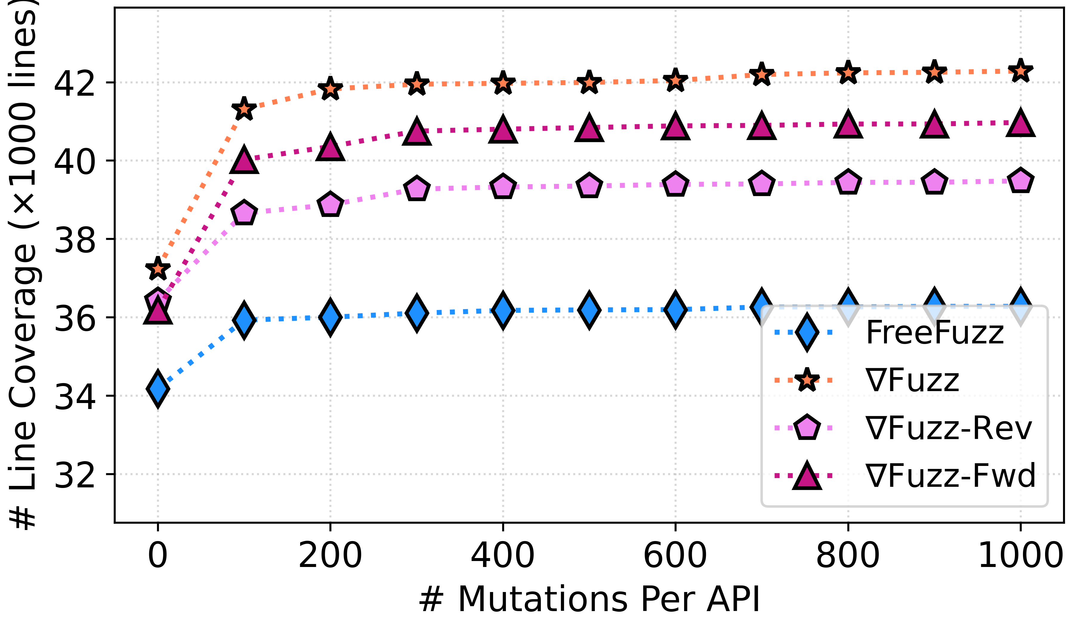
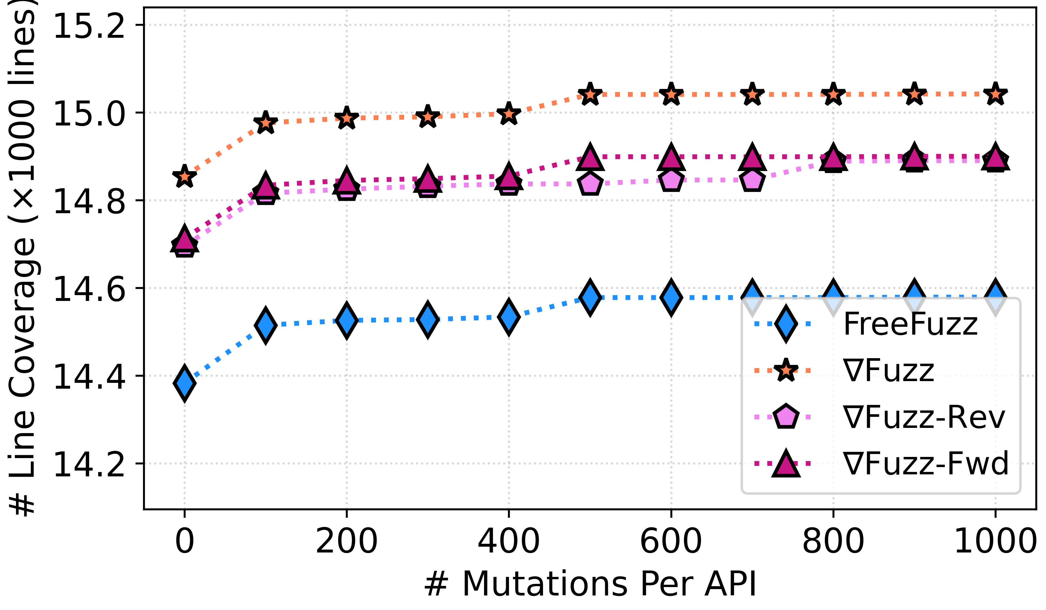
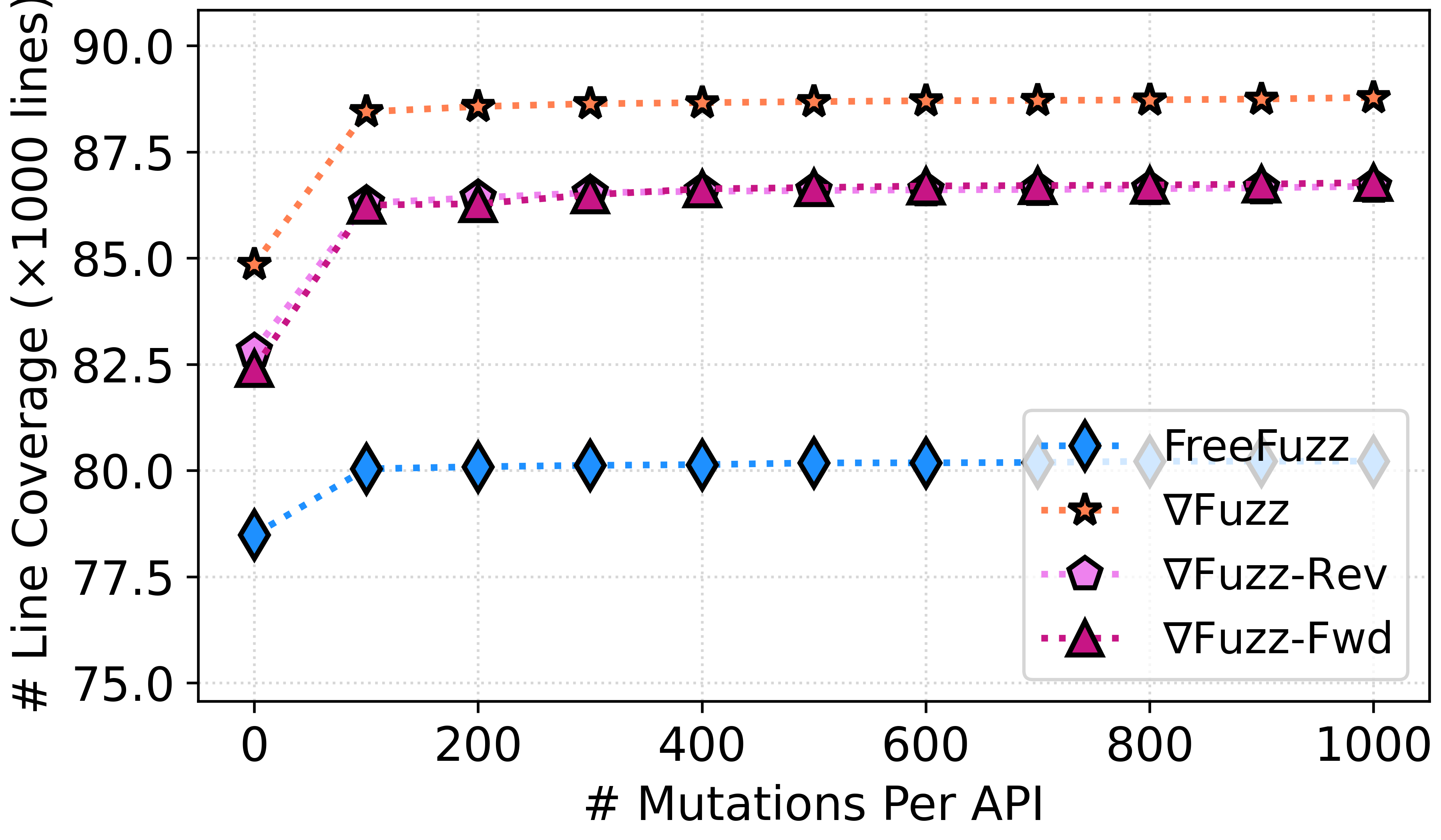
Figure 11 shows the coverage results, where the $x$ axis is the number of mutants generated for each API (from 100 to 1000 with the interval of 100), while the $y$ axis is the overall line coverage achieved. Note that the code coverage achieved by running the seed inputs in the FreeFuzz database (without any mutation) is the start point for each line.For C++ coverage, we can observe that $\nabla$ Fuzz outperforms FreeFuzz significantly on both PyTorch and TensorFlow, with an improvement of 22.4%/16.6% respectively. Note that such an improvement is highly valuable as the additionally covered code is mostly about the crucial AD mechanism. For Python coverage, $\nabla$ Fuzz still outperforms FreeFuzz, but with a smaller improvement than C++. The possible reason could be that the crucial AD functionality of DL libraries is mainly implemented in C++, e.g., the official material of PyTorch said, “Autograd is a hotspot for PyTorch performance, so most of the heavy lifting is implemented in C++” [63].

Table VI further presents the time cost and overall system coverage rate for FreeFuzz and $\nabla$ Fuzz. The time cost of $\nabla$ Fuzz is higher than FreeFuzz due to the additional gradient computation (mostly on the expensive second-order gradients). Meanwhile, we can find that the $\nabla$ Fuzz only running the seed inputs in the database (Row “ $\nabla$ Fuzz (seed only)”) still outperforms FreeFuzz in terms of code coverage even with less time. Moreover, $\nabla$ Fuzz achieves decent system coverage rates, e.g., 25.8% for the entire PyTorch C++ codebase and 33.3% for the entire TensorFlow Python codebase.

We also compare $\nabla$ Fuzz with Muffin. Since Muffin does not support PyTorch, JAX, or OneFlow, we conduct this comparison on TensorFlow only. We run Muffin with its default setting (which takes 6.8h). For a fair comparison, we run $\nabla$ Fuzz by setting the number of mutants for each API to 150, so it can finish within 6.8h. As shown in Table VII, with slightly less execution time (6.1h), $\nabla$ Fuzz already substantially outperforms Muffin in both code and API coverage. In fact, even only running the seed API inputs without mutation with our AD oracle (taking only 2.9h) is sufficient to outperform Muffin in terms of C++ and Python coverage. This is because $\nabla$ Fuzz can cover much more APIs and more AD modes, while Muffin only considers reverse mode AD on a small set of APIs. More precisely, Muffin only covers 79 TensorFlow APIs, while $\nabla$ Fuzz can cover 1902. This is because Muffin only considers a set of predefined high-level layer APIs [29] for model generation. Meanwhile, Muffin can already achieve decent code coverage (albeit lower than $\nabla$ Fuzz) because such high-level APIs will use various low-level operations.

TABLE VI: Comparison with FreeFuzz

	PyTorch			TensorFlow
	C++ Cov	Python Cov	Time	C++ Cov	Python Cov	Time
FreeFuzz	70639 (21.1%)	14579 (13.9%)	3.1h	36279 (9.77%)	80220 (30.1%)	3.9h
$\nabla$ Fuzz	86459 (25.8%)	15042 (14.3%)	25.7h	42284 (11.4%)	88783 (33.3%)	24.3h
$\nabla$ Fuzz (seed only)	79808 (23.4%)	14854 (14.1%)	1.4h	37233 (10.0%)	84848 (31.9%)	2.9h

TABLE VII: Comparison with Muffin

	C++ Coverage	Python Coverage	# Covered API	Time
$\nabla$ Fuzz	41625 (11.21%)	88524 (33.24%)	1902	6.1h
Muffin	36884 (9.94%)	78754 (29.57%)	79	6.8h

VI-B RQ2: Different Components of Test Oracles

VI-B1 Impact on Bug Detection

TABLE VIII: Scenario distribution of confirmed bugs

	Direct	AD			ND
	Invocation	All	Rev-Only	Fwd-Only	ND
PyTorch	11	64	33	9	2
TensorFlow	3	18	5	4	2
JAX	3	20	3	1	0
OneFlow	16	5	5	N/A	N/A
Total	33	107	46	14	4

In Table VIII, we categorize all confirmed bugs based on which execution scenarios they are located in, such as direct invocation, AD, and ND. Among the bugs in AD, Column “All” displays the total number of bugs located in AD, while Column “Rev-Only”/“Fwd-Only” presents the number of bugs only appearing in reverse/forward mode respectively.That said, 47 (107-46-14) bugs are in both reverse and forward AD modes. From this table, we can conclude that most of the bugs detected by $\nabla$ Fuzz are related to our main target AD, showing the strength of $\nabla$ Fuzz in fuzzing AD for DL libraries. One interesting fact is that we detect more bugs in direct invocation than AD in OneFlow. This may be because OneFlow was not tested by the original FreeFuzz work and only supports reverse-mode AD. Furthermore, we detect more reverse mode unique bugs than forward mode since reverse mode is more widely implemented in DL libraries.As mentioned in §V-A2, we directly leverage the ND computation/comparison APIs in PyTorch, TensorFlow and JAX. It turns out we can even detect 4 bugs in such APIs.

TABLE IX: Symptoms of confirmed bugs

	Output	Gradient Total	1st-order	2nd-order
PyTorch	31	46	44	2
TensorFlow	4	19	17	2
JAX	14	9	8	1
OneFlow	16	5	2	3
Total	65	79	71	8

We also categorize all the confirmed bugs by how they were detected in Table IX, e.g., the bugs are found by inconsistent outputs (Column “Output”) or gradients (Column “Gradient Total”). We further split the bugs detected by the gradient into checks for the first-order gradients (Column “1st-order”) and second-order gradients (Column “2nd-order”). We can observe that more than half bugs are detected by inconsistent gradients, showing the importance of gradient oracles. Plus, most of the gradient-related bugs are first-order. This is because the first- and second-order gradient computations often share part of the implementation, and any bug in the former will prevent $\nabla$ Fuzz from testing the latter. Notably, $\nabla$ Fuzz can still detect 8 bugs using the second-order gradient check, showing the generality of our approach. More interestingly, 65 bugs are revealed by discrepant outputs, indicating that the AD mechanism could even affect normal DL API forward computation!

VI-B2 Impact on Code Coverage

To study the impact of execution scenarios on code coverage, we have two $\nabla$ Fuzz variants: $\nabla$ Fuzz-Rev (disabling reverse mode AD) and $\nabla$ Fuzz-Fwd (disabling forward mode AD). We skip the coverage analysis of ND since it is typically implemented based on the basic direct API invocations and can hardly cover new code.Figure 11 also presents the research findings for the studied variants with various amounts of mutations for each API. We can observe that the reverse mode AD occupies a larger portion of the DL library implementation than the forward mode because $\nabla$ Fuzz-Fwd outperforms $\nabla$ Fuzz-Rev in terms of code coverage. This complies with the truth that reverse mode AD is the main technique used in DL systems.More importantly, we can also observe that the code coverage of both reverse and forward mode AD is not negligible, indicating the necessity of considering both of them for DL library fuzzing.

VI-C RQ3: FPR and Effectiveness of the Filtering Strategies

Table X shows the results of the FPR, which is categorized based on the checks. Column “Output”/“Gradient” shows the FPR of output/gradient check respectively. Column “Total” is the overall FPR of our technique. Under Column “Gradient”, Column “All” is the FPR when both filtering strategies are used, and Column “N/A” is the FPR without any strategy. Column “Diff”/“Precision” presents the FPR with only the differentiability/precision strategy, respectively. From the table, we can observe that the overall FPR of $\nabla$ Fuzz is only around 20%, implying the efficacy of $\nabla$ Fuzz. Notably, our filtering strategies do not remove any true bug mistakenly, as confirmed by our manual check for all reported inconsistencies. Besides, the FPR of the gradient oracle with filtering (22.4%) is much lower than without it (66.7%), showing the effectiveness of our filtering strategies.Also, we can observe that both filtering strategies are effective in reducing FPR. More precisely, the differentiability strategy is more helpful than the precision strategy, especially in OneFlow, where the latter cannot help reduce any false positives. Moreover, the FPR of the output oracle is lower than the gradient oracle (even after filtering). The main reason is that API outputs should not be affected by different AD modes, while the computed gradients can be slightly different across reverse-/forward-mode AD and ND due to different underlying implementations.

We further evaluate the impact of hyper-parameters, sampling number $N$ (default 5) and distance $\delta$ (default 10^-4). The study is conducted on our default subjects, PyTorch and TensorFlow, due to the space limit.For the impact of sampling number $N$ , we run our experiments with different $N$ values of 1, 2, 5, 10 as shown in Table XI. The choice of $N$ contributes little to the FPR of gradient oracle since all of them are close. Plus, the FPR decreases as $N$ increases, as more neighbors to compare implies more false positives will be filtered. However, the time cost will also increase as $N$ increases (e.g. the time cost of $N$ = 10 is about 1.5X higher than that of $N$ = 5). Thus, $N$ = 5 is a trade-off between the FPR and the time cost.

As for the impact of distance $\delta$ , we run with different $\delta$ values of 10^-1, 10^-2, 10^-3, 10^-4, 10^-5. The result is shown in Table XII. First, the FPR decreases as $\delta$ increases. This is because the neighbor with a farther distance is more likely to have a different gradient, causing some false positives to be filtered. However, it may also exclude the real bugs since the large distance may cause the gradient to change dramatically even at differentiable points. For example, in PyTorch, $\delta$ = 10^-3 could filter out 2 true positives. We choose $\delta$ = 10^-4 as our default setting since it does not filter out any true positives.

VI-D Threats to Validity

The main threat to internal validity lies in the implementation of $\nabla$ Fuzz. The authors have thoroughly tested and reviewed the code of $\nabla$ Fuzz to lessen the threat. The threats to external validity mainly lie in the evaluation benchmarks used. We evaluated $\nabla$ Fuzz on four of the most widely-used and actively-maintained DL libraries to confirm the generality of our approach. Moreover, we adopt detected bugs, code coverage, false positive analysis, and execution time to reduce the threats to construct validity for the metrics used.

TABLE X: False positive rate (FPR)

	Output	Gradient				Total
	Output	All	Diff	Precision	N/A	Total
PyTorch	19.3%	21.2%	25.5%	57.3%	61.9%	20.7%
TensorFlow	8.3%	21.1%	34.8%	46.4%	53.1%	16.1%
JAX	11.1%	21.0%	58.1%	68.6%	78.2%	17.3%
OneFlow	12.5%	25.0%	25.0%	64.0%	64.0%	20.0%
Total	15.0%	22.4%	37.7%	59.8%	66.7%	19.3%

TABLE XI: FPR of gradient oracle w.r.t

N

Sampling Number $N$	1	2	5	10
PyTorch	23.6%	22.6%	21.2%	21.2%
TensorFlow	21.1%	21.1%	21.1%	21.1%

TABLE XII: FPR of gradient oracle w.r.t

\delta

Sampling Distance $\delta$	$10^{-1}$	$10^{-2}$	$10^{-3}$	$10^{-4}$	$10^{-5}$
PyTorch	17.2%	19.3%	20.4%	21.2%	22.9%
TensorFlow	7.1%	18.8%	18.8%	21.1%	21.1%

VII Related Work

CRADLE [25] is a pioneering work on DL library fuzzing, which leverages differential testing to detect bugs by running existing DL models on different low-level DL libraries of Keras [26]. AUDEE [27] and LEMON [28] further augment CRADLE by applying search-based mutation strategies on existing DL models to cover more library code. While LEMON adopted advanced mutation rules (e.g., layer addition), it still only covers a small set of APIs [30] due to its strict mutation rules, e.g., an API cannot be added/removed in the model unless its input and output tensor shapes are identical. More importantly, these techniques focus on the inference phase of DL models, and thus cannot detect any AD bug. To mitigate this, the recent Muffin work [29] is proposed to detect bugs in both inference and training phases by generating DL models via a top-down approach. While Muffin can potentially cover reverse-mode AD, it can only cover a small number of APIs in specific libraries, and cannot detect any confirmed AD bug (please see §I for detailed discussion). More recently, NNSmith [64] leverages lightweight formal specifications to model each operator, and generates diverse and valid models via symbolic constraint solving. While NNSmith has been demonstrated to be state-of-the-art model-level DL library fuzzer, it still only targets the inference phase, while our work is orthogonal and can be applied to further augment NNSmith.

Besides leveraging DL models for testing DL libraries, researchers have also investigated directly fuzzing DL library APIs. Meanwhile, DL library APIs are often exposed in Python, a dynamically typed language, making it hard even to determine the input types for DL APIs.To overcome this issue, Predoo [65] requires manually setting up API arguments for DL library fuzzing, and thus was only evaluated on 7 TensorFlow APIs (due to the manual efforts). More recently, DocTer [31] synthesizes rules to extract API input constraints from DL library documentations, and then generates API inputs based on the constraints. However, it still requires manual efforts for annotating 30% of API parameters. Different from above work, FreeFuzz [30] is a fully-automated technique for DL library API fuzzing. More specifically, FreeFuzz automatically tracks API inputs when running code mined from the open-source; additional mutations are performed to generate more inputs based on tracked seed API inputs. Another line of recent work designs other test oracles for DL libraries, e.g., DeepREL [53] automatically infers relational APIs (e.g., the APIs that should return the same values/statuses when given the same inputs) as the oracle to detect inconsistency bugs for DL libraries, while EAGLE [41] uses equivalent graphs to differentially test DL APIs. While effective, none of the existing API-level techniques targeted the crucial AD engines in DL libraries.

Different from the above model- and API-level fuzzers which struggle to cover valid API sequences for a large number of APIs (due to complicated input/shape constraints), the very recent LLMFuzz work [66] proposes to directly apply modern Large Language Models (LLMs) [67] to generate diverse DL API sequences. The insight is that LLMs can implicitly learn intricate DL API constraints from DL programs in their massive training corpora. LLMFuzz demonstrates, for the first time, that modern LLMs (e.g., Codex [67]) can be directly leveraged for end-to-end fuzzing of real-world systems. $\nabla$ Fuzz is also orthogonal to LLMFuzz and can be further applied to enhance its oracle support.

VIII Conclusion

$\nabla$ Fuzz is the first approach specifically targeting the AD engine in DL libraries, which is a crucial component of any DL system. It leverages different execution scenarios as test oracles to test first- and high-order gradients and incorporates an automated filter to reduce the false positives caused by numerical instability. The evaluation of $\nabla$ Fuzz on PyTorch, TensorFlow, JAX and OneFlow shows that $\nabla$ Fuzz can detect 173 bugs in total, with 144 confirmed by developers (117 of which are previously unknown) and 38 already fixed. Notably, $\nabla$ Fuzz contributed 58.3% (7/12) of all high-priority AD bugs for PyTorch and JAX during a two-month period.

Data Availability: Our code and data are available at [68].

Acknowledgments

This work was partially supported by NSF grants CCF-2131943, and CCF-2141474. We also acknowledge support from Google and Meta.

References

[1] T. Young, D. Hazarika, S. Poria, and E. Cambria, “Recent trends in deep learning based natural language processing,” ieee Computational intelligenCe magazine, vol. 13, no. 3, pp. 55–75, 2018.
[2] A. Esteva, A. Robicquet, B. Ramsundar, V. Kuleshov, M. DePristo, K. Chou, C. Cui, G. Corrado, S. Thrun, and J. Dean, “A guide to deep learning in healthcare,” Nature medicine, vol. 25, no. 1, pp. 24–29, 2019.
[3] J. Jumper, R. Evans, A. Pritzel, T. Green, M. Figurnov, O. Ronneberger, K. Tunyasuvunakool, R. Bates, A. Žídek, A. Potapenko, A. Bridgland, C. Meyer, S. A. A. Kohl, A. J. Ballard, A. Cowie, B. Romera-Paredes, S. Nikolov, R. Jain, J. Adler, T. Back, S. Petersen, D. Reiman, E. Clancy, M. Zielinski, M. Steinegger, M. Pacholska, T. Berghammer, S. Bodenstein, D. Silver, O. Vinyals, A. W. Senior, K. Kavukcuoglu, P. Kohli, and D. Hassabis, “Highly accurate protein structure prediction with AlphaFold,” Nature, vol. 596, no. 7873, pp. 583–589, 2021.
[4] A. Goffi, A. Gorla, M. D. Ernst, and M. Pezzè, “Automatic generation of oracles for exceptional behaviors,” in Proceedings of the 25th international symposium on software testing and analysis, 2016, pp. 213–224.
[5] X. Gu, H. Zhang, and S. Kim, “Deep code search,” in 2018 IEEE/ACM 40th International Conference on Software Engineering (ICSE). IEEE, 2018, pp. 933–944.
[6] X. Li, W. Li, Y. Zhang, and L. Zhang, “Deepfl: Integrating multiple fault diagnosis dimensions for deep fault localization,” in Proceedings of the 28th ACM SIGSOFT International Symposium on Software Testing and Analysis, 2019, pp. 169–180.
[7] Y. Li, S. Wang, and T. N. Nguyen, “Dlfix: Context-based code transformation learning for automated program repair,” in Proceedings of the ACM/IEEE 42nd International Conference on Software Engineering, 2020, pp. 602–614.
[8] C. S. Xia, Y. Wei, and L. Zhang, “Automated program repair in the era of large pre-trained language models,” in ICSE, 2023, to appear.
[9] C. S. Xia and L. Zhang, “Less training, more repairing please: Revisiting automated program repair via zero-shot learning,” in FSE, 2022.
[10] Garcia, Joshua and Feng, Yang and Shen, Junjie and Almanee, Sumaya and Xia, Yuan and Chen, and Qi Alfred, “A comprehensive study of autonomous vehicle bugs,” in Proceedings of the ACM/IEEE 42nd International Conference on Software Engineering, 2020, pp. 385–396.
[11] D. Shriver, S. Elbaum, and M. Dwyer, “Artifact: reducing dnn properties to enable falsification with adversarial attacks,” in 2021 IEEE/ACM 43rd International Conference on Software Engineering: Companion Proceedings (ICSE-Companion). IEEE, 2021, pp. 162–163.
[12] N. Akhtar and A. Mian, “Threat of adversarial attacks on deep learning in computer vision: A survey,” Ieee Access, vol. 6, pp. 14 410–14 430, 2018.
[13] N. Carlini, A. Athalye, N. Papernot, W. Brendel, J. Rauber, D. Tsipras, I. Goodfellow, A. Madry, and A. Kurakin, “On evaluating adversarial robustness,” arXiv preprint arXiv:1902.06705, 2019.
[14] D. Gopinath, M. Zhang, K. Wang, I. B. Kadron, C. Pasareanu, and S. Khurshid, “Symbolic execution for importance analysis and adversarial generation in neural networks,” in 2019 IEEE 30th International Symposium on Software Reliability Engineering (ISSRE). IEEE, 2019, pp. 313–322.
[15] A. Madry, A. Makelov, L. Schmidt, D. Tsipras, and A. Vladu, “Towards deep learning models resistant to adversarial attacks,” arXiv preprint arXiv:1706.06083, 2017.
[16] S.-M. Moosavi-Dezfooli, A. Fawzi, and P. Frossard, “Deepfool: a simple and accurate method to fool deep neural networks,” in Proceedings of the IEEE conference on computer vision and pattern recognition, 2016, pp. 2574–2582.
[17] N. Papernot, P. McDaniel, S. Jha, M. Fredrikson, Z. B. Celik, and A. Swami, “The limitations of deep learning in adversarial settings,” in 2016 IEEE European symposium on security and privacy (EuroS&P). IEEE, 2016, pp. 372–387.
[18] K. Pei, Y. Cao, J. Yang, and S. Jana, “Deepxplore: Automated whitebox testing of deep learning systems,” in proceedings of the 26th Symposium on Operating Systems Principles, 2017, pp. 1–18.
[19] M. Yan, J. Chen, X. Zhang, L. Tan, G. Wang, and Z. Wang, “Exposing numerical bugs in deep learning via gradient back-propagation,” in Proceedings of the 29th ACM Joint Meeting on European Software Engineering Conference and Symposium on the Foundations of Software Engineering, 2021, pp. 627–638.
[20] H. Zhang, Z. Fu, G. Li, L. Ma, Z. Zhao, H. Yang, Y. Sun, Y. Liu, and Z. Jin, “Towards robustness of deep program processing models—detection, estimation, and enhancement,” ACM Transactions on Software Engineering and Methodology (TOSEM), vol. 31, no. 3, pp. 1–40, 2022.
[21] Z. Yang, J. Shi, J. He, and D. Lo, “Natural attack for pre-trained models of code,” in Proceedings of the 44th International Conference on Software Engineering. New York, NY, USA: Association for Computing Machinery, 2022, p. 1482–1493. [Online]. Available: https://doi.org/10.1145/3510003.3510146
[22] J. Cao, B. Chen, C. Sun, L. Hu, and X. Peng, “Characterizing performance bugs in deep learning systems,” arXiv preprint arXiv:2112.01771, 2021.
[23] Y. Zhang, L. Ren, L. Chen, Y. Xiong, S.-C. Cheung, and T. Xie, “Detecting numerical bugs in neural network architectures,” in Proceedings of the 28th ACM Joint Meeting on European Software Engineering Conference and Symposium on the Foundations of Software Engineering, 2020, pp. 826–837.
[24] S. Lagouvardos, J. Dolby, N. Grech, A. Antoniadis, and Y. Smaragdakis, “Static analysis of shape in tensorflow programs,” in 34th European Conference on Object-Oriented Programming (ECOOP 2020). Schloss Dagstuhl-Leibniz-Zentrum für Informatik, 2020.
[25] H. V. Pham, T. Lutellier, W. Qi, and L. Tan, “CRADLE: Cross-Backend Validation to Detect and Localize Bugs in Deep Learning Libraries,” in 2019 IEEE/ACM 41st International Conference on Software Engineering (ICSE), 2019, pp. 1027–1038.
[26] “Keras,” https://keras.io, 2015.
[27] Q. Guo, X. Xie, Y. Li, X. Zhang, Y. Liu, X. Li, and C. Shen, “Audee: Automated testing for deep learning frameworks,” in 2020 35th IEEE/ACM International Conference on Automated Software Engineering (ASE). IEEE, 2020, pp. 486–498.
[28] Z. Wang, M. Yan, J. Chen, S. Liu, and D. Zhang, “Deep learning library testing via effective model generation,” in Proceedings of the 28th ACM Joint Meeting on European Software Engineering Conference and Symposium on the Foundations of Software Engineering, 2020, pp. 788–799.
[29] J. Gu, X. Luo, Y. Zhou, and X. Wang, “Muffin: Testing deep learning libraries via neural architecture fuzzing,” in 2022 IEEE/ACM 44th International Conference on Software Engineering (ICSE). Los Alamitos, CA, USA: IEEE Computer Society, may 2022, pp. 1418–1430. [Online]. Available: https://doi.ieeecomputersociety.org/10.1145/3510003.3510092
[30] A. Wei, Y. Deng, C. Yang, and L. Zhang, “Free lunch for testing: Fuzzing deep-learning libraries from open source,” in 2022 IEEE/ACM 44th International Conference on Software Engineering (ICSE), 2022, pp. 995–1007.
[31] D. Xie, Y. Li, M. Kim, H. V. Pham, L. Tan, X. Zhang, and M. W. Godfrey, “Docter: Documentation-guided fuzzing for testing deep learning api functions,” in Proceedings of the 31st ACM SIGSOFT International Symposium on Software Testing and Analysis, 2022, to appear.
[32] B. van Merrienboer, O. Breuleux, A. Bergeron, and P. Lamblin, “Automatic differentiation in ml: Where we are and where we should be going,” in NeurIPS, 2018.
[33] Wikipedia contributors, “Backpropagation — Wikipedia, the free encyclopedia,” https://en.wikipedia.org/w/index.php?title=Backpropagation&oldid=1104872812, 2022.
[34] S. Zhang, S. Roller, N. Goyal, M. Artetxe, M. Chen, S. Chen, C. Dewan, M. Diab, X. Li, X. V. Lin et al., “Opt: Open pre-trained transformer language models,” arXiv preprint arXiv:2205.01068, 2022.
[35] P. Gasti, G. Tsudik, E. Uzun, and L. Zhang, “Dos and ddos in named data networking,” in 2013 22nd International Conference on Computer Communication and Networks (ICCCN), 2013, pp. 1–7.
[36] “Definition of Xlogy from Pytorch official documentation,” https://pytorch.org/docs/stable/generated/torch.nn.KLDivLoss.html, 2022.
[37] “Keras 2.3.0 release,” https://github.com/keras-team/keras/releases/tag/2.3.0, 2019.
[38] “FreeFuzz Repository,” https://github.com/ise-uiuc/FreeFuzz, 2022.
[39] A. G. Baydin, B. A. Pearlmutter, A. Radul, and J. M. Siskind, “Automatic differentiation in machine learning: a survey,” J. Mach. Learn. Res., vol. 18, pp. 153:1–153:43, 2017.
[40] Wikipedia contributors, “Hessian matrix — Wikipedia, the free encyclopedia,” https://en.wikipedia.org/w/index.php?title=Hessian_matrix&oldid=1107031412, 2022.
[41] J. Wang, T. Lutellier, S. Qian, H. V. Pham, and L. Tan, “Eagle: Creating equivalent graphs to test deep learning libraries,” 2022.
[42] Wikipedia contributors, “Jacobian matrix and determinant — Wikipedia, the free encyclopedia,” https://en.wikipedia.org/w/index.php?title=Jacobian_matrix_and_determinant&oldid=1104898576, 2022.
[43] Wikipedia contributors , “Tangent space — Wikipedia, the free encyclopedia,” https://en.wikipedia.org/w/index.php?title=Tangent_space&oldid=1091055882, 2022.
[44] R. L. Burden, J. D. Faires, and A. M. Burden, Numerical analysis. Cengage learning, 2015.
[45] “Definition of Dynamic_index_in_dim from JAX official documentation,” https://jax.readthedocs.io/en/latest/_autosummary/jax.lax.dynamic_index_in_dim.html, 2022.
[46] “Definition of Trace from Pytorch official documentation,” https://pytorch.org/docs/stable/generated/torch.trace.html, 2022.
[47] “Definition of Hardshrink from Pytorch official documentation,” https://pytorch.org/docs/stable/generated/torch.nn.Hardshrink.html, 2022.
[48] “Definition of Pow from JAX official documentation,” https://jax.readthedocs.io/en/latest/_autosummary/jax.lax.pow.html, 2022.
[49] Wikipedia contributors, “Differentiable function — Wikipedia, the free encyclopedia,” https://en.wikipedia.org/w/index.php?title=Differentiable_function&oldid=1101867284, 2022.
[50] “Definition of Sum from Pytorch official documentation,” https://pytorch.org/docs/stable/generated/torch.sum.html, 2022.
[51] J. Bradbury, R. Frostig, P. Hawkins, M. J. Johnson, C. Leary, D. Maclaurin, G. Necula, A. Paszke, J. VanderPlas, S. Wanderman-Milne, and Q. Zhang, “JAX: composable transformations of Python+NumPy programs,” http://github.com/google/jax, 2018.
[52] J. Yuan, X. Li, C. Cheng, J. Liu, R. Guo, S. Cai, C. Yao, F. Yang, X. Yi, C. Wu, H. Zhang, and J. Zhao, “Oneflow: Redesign the distributed deep learning framework from scratch,” 2021.
[53] Y. Deng, C. Yang, A. Wei, and L. Zhang, “Fuzzing deep-learning libraries via automated relational api inference,” in 30th ACM Joint European Software Engineering Conference and Symposium on the Foundations of Software Engineering (ESEC/FSE), 2022.
[54] T. Su, Y. Yan, J. Wang, J. Sun, Y. Xiong, G. Pu, K. Wang, and Z. Su, “Fully automated functional fuzzing of android apps for detecting non-crashing logic bugs,” Proceedings of the ACM on Programming Languages, vol. 5, no. OOPSLA, pp. 1–31, 2021.
[55] W. You, X. Wang, S. Ma, J. Huang, X. Zhang, X. Wang, and B. Liang, “Profuzzer: On-the-fly input type probing for better zero-day vulnerability discovery,” in 2019 IEEE symposium on security and privacy (SP). IEEE, 2019, pp. 769–786.
[56] A. F. Donaldson, H. Evrard, A. Lascu, and P. Thomson, “Automated testing of graphics shader compilers,” Proceedings of the ACM on Programming Languages, vol. 1, no. OOPSLA, pp. 1–29, 2017.
[57] J. Liu, Y. Wei, S. Yang, Y. Deng, and L. Zhang, “Coverage-guided tensor compiler fuzzing with joint ir-pass mutation,” Proc. ACM Program. Lang., vol. 6, no. OOPSLA1, apr 2022. [Online]. Available: https://doi.org/10.1145/3527317
[58] “GCOV,” https://gcc.gnu.org/onlinedocs/gcc/Gcov.html, 2022.
[59] “Coverage.py,” https://github.com/nedbat/coveragepy, 2022.
[60] “Definition of RReLU from Pytorch official documentation,” https://pytorch.org/docs/stable/generated/torch.nn.RReLU.html, 2022.
[61] “Definition of Sinc from JAX official documentation,” https://jax.readthedocs.io/en/latest/_autosummary/jax.numpy.sinc.html, 2022.
[62] Wikipedia contributors, “Bfloat16 floating-point format — Wikipedia, the free encyclopedia,” https://en.wikipedia.org/w/index.php?title=Bfloat16_floating-point_format&oldid=1041556217, 2021.
[63] “Autograd from Pytorch official material,” https://github.com/pytorch/pytorch/blob/master/torch/csrc/autograd/README.md, 2022.
[64] J. Liu, J. Lin, F. Ruffy, C. Tan, J. Li, A. Panda, and L. Zhang, “Nnsmith: Generating diverse and valid test cases for deep learning compilers,” in Proceedings of the 28th ACM International Conference on Architectural Support for Programming Languages and Operating Systems, Volume 2, ser. ASPLOS 2023. New York, NY, USA: Association for Computing Machinery, 2023, p. 530–543. [Online]. Available: https://doi.org/10.1145/3575693.3575707
[65] X. Zhang, N. Sun, C. Fang, J. Liu, J. Liu, D. Chai, J. Wang, and Z. Chen, “Predoo: precision testing of deep learning operators,” in Proceedings of the 30th ACM SIGSOFT International Symposium on Software Testing and Analysis, 2021, pp. 400–412.
[66] Y. Deng, C. S. Xia, H. Peng, C. Yang, and L. Zhang, “Fuzzing deep-learning libraries via large language models,” in Proceedings of the 32nd ACM SIGSOFT International Symposium on Software Testing and Analysis, ser. ISSTA 2023, 2023.
[67] M. Chen, J. Tworek, H. Jun, Q. Yuan, H. P. d. O. Pinto, J. Kaplan, H. Edwards, Y. Burda, N. Joseph, G. Brockman et al., “Evaluating large language models trained on code,” arXiv preprint arXiv:2107.03374, 2021.
[68] “ $\nabla$ Fuzz Repository,” https://github.com/ise-uiuc/NablaFuzz, 2022.