Quantum Computation of Frequency-Domain Molecular Response Properties Using a Three-Qubit iToffoli Gate
Abstract
The quantum computation of molecular response properties on near-term quantum hardware is a topic of significant interest. While computing time-domain response properties is in principle straightforward due to the natural ability of quantum computers to simulate unitary time evolution, circuit depth limitations restrict the maximum time that can be simulated and hence the extraction of frequency-domain properties. Computing properties directly in the frequency domain is therefore desirable, but the circuits require large depth when the typical hardware gate set consisting of single- and two-qubit gates is used. Here, we report the experimental quantum computation of the response properties of diatomic molecules directly in the frequency domain using a three-qubit iToffoli gate, enabling a reduction in circuit depth by a factor of two. We show that the molecular properties obtained with the iToffoli gate exhibit comparable or better agreement with theory than those obtained with the native CZ gates. Our work is among the first demonstrations of the practical usage of a native multi-qubit gate in quantum simulation, with diverse potential applications to the simulation of quantum many-body systems on near-term digital quantum computers.
Introduction
A primary goal of emerging quantum computing technologies is to enable the simulation of quantum many-body systems that are challenging for classical computers Feynman 1982; Lloyd 1996; Georgescu et al. 2014. Early experimental demonstrations of quantum simulation algorithms have focused on computing ground- and excited-state energies of small molecules Peruzzo et al. 2014; O’Malley et al. 2016; Kandala et al. 2017; Colless et al. 2018 or few-site spin Kandala et al. 2017 and fermionic models Barends et al. 2015. More recently, the scale of quantum simulation experiments has increased in terms of numbers of qubits, diversity of gate sets, and complexity of algorithms, as manifested in simulation of models based on real molecules and materials Arute et al. 2020; Tazhigulov et al. 2022; Stanisic et al. 2022, various phases of matter such as thermal Motta et al. 2019; Francis et al. 2021, topological Satzinger et al. 2021; Tan et al. 2021 and many-body localized states mi_ 2022; Karamlou et al. 2022, as well as holographic quantum simulation using quantum tensor networks Niu et al. 2022; Chertkov et al. 2022; Gibbs et al. 2022. As quantum advantages in random sampling have been established on quantum hardware Arute et al. 2019; Wu et al. 2021, focus has turned to the experimental demonstration of quantum advantages in problems of physical significance Daley et al. 2022.
For applications in chemistry and physics, the calculation of the response properties of molecules and materials is of substantial interest Cao et al. 2019; McArdle et al.; Bauer et al. 2020. Investigating response properties in the electronic structure theory framework involves calculating quantities such as the one-particle Green’s function von Nissen et al. 1984 and density-density response functions Ullrich 2019, which provide insight into interpreting experimental spectroscopic measurements Damascelli et al. 2003. Response properties of molecules and materials can be determined either in time domain or in frequency domain. Due to the natural ability of quantum computers to simulate time evolution Feynman 1982; Lloyd 1996, near-term algorithms to compute time-domain response properties have been carried out on quantum hardware Chiesa et al. 2019; Francis et al. 2020; Sun et al. 2021. However, computing the frequency-domain response from the time-domain response using the typical gate set available on hardware requires a time duration that exceeds the circuit depth limitations of near-term quantum computers.
An alternative approach to determine these response properties is by computing them directly in the frequency domain. Frequency-domain algorithms generally involve obtaining the ground- and excited-state energies as well as the transition amplitudes between the ground state and the excited states. Although there are established methods to obtain ground- and excited-state energies on quantum computers McClean et al. 2017; Nakanishi et al. 2019; Parrish et al. 2019; Higgott et al. 2019; Jones et al. 2019, calculating transition amplitudes is less straightforward. Various schemes including variational quantum simulation Endo et al. 2020; Chen et al., quantum subspace expansion Jamet et al. 2022 and quantum linear algebra Cai et al. 2020 to determine frequency-domain response properties have been proposed. However, the accuracy of variational methods depends on the quality of the ansatz, quantum subspace expansion is susceptible to numerical instabilities from basis linear dependence, and quantum linear algebra is out of reach for near-term quantum hardware. Recently, a non-variational scheme amenable to near-term hardware implementation has been proposed Kosugi and Matsushita 2020a; Kosugi and Matsushita 2020b. This scheme constructs the electron-added and electron-removed states simultaneously by exploiting the probabilistic nature of the linear combination of unitaries (LCU) algorithm Childs and Wiebe. Nevertheless, this LCU-based algorithm has not yet been demonstrated on quantum hardware due to the lack of efficient implementations of the multi-qubit gates.
In this work, we experimentally demonstrate the calculation of frequency-domain response properties of diatomic molecules using a recently reported high-fidelity three-qubit iToffoli gate Kim et al. 2022 to implement the LCU circuits on a superconducting quantum processor. The multi-controlled gates present in the original LCU algorithm are decomposed either with iToffoli gates or with CZ gates. We calculate transition amplitudes between the ground state and the -electron or -electron states of NaH and KH molecules restricted to the highest occupied and lowest unoccupied molecular orbitals (HOMO and LUMO). The transition amplitudes are then used to construct spectral functions and density-density response functions of the diatomic molecules. We apply error mitigation techniques including randomized compiling (RC) Wallman and Emerson 2016; Hashim et al. 2021 during circuit construction, and McWeeny purification McWeeny 1960 during postprocessing, both of which result in marked improvement of the experimental observables. The observables obtained from the reduced-depth circuits with iToffoli decomposition show comparable or better agreement with theory compared to the observables from circuits with CZ decomposition, despite incomplete Pauli twirling in the randomized compiling procedure applied to the iToffoli gate. Our results pave the way for the application of multi-qubit gates for quantum chemistry and related quantum simulation applications on near-term quantum hardware.
Results
Quantum Algorithm for Transition Amplitudes of Diatomic Molecules
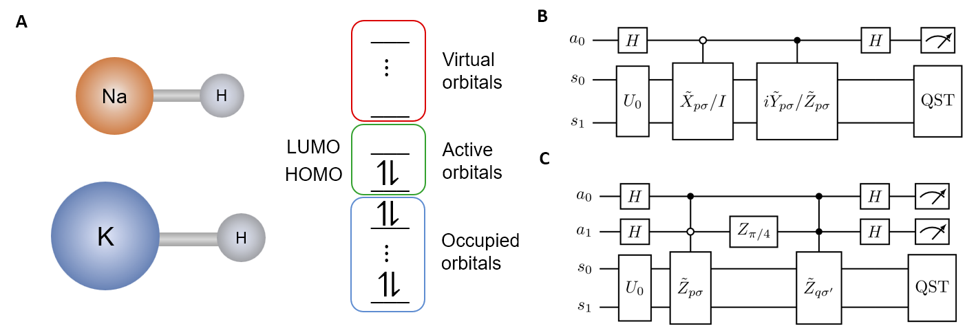
We consider the HOMO-LUMO models of the diatomic molecules NaH and KH as shown in Fig. 1 (see Methods). Such molecular models with reduced active space have been used in benchmarking quantum chemistry methods on quantum computers Yeter‐Aydeniz et al. 2021. The HOMO-LUMO model generates two spatial orbitals or equivalently four spin orbitals, which correspond to four qubits after Jordan-Wigner transformation Jordan and Wigner 1928. To reduce quantum resources, we exploit the number symmetry in each spin sector to reduce the number of qubits from four to two using a qubit-tapering technique Bravyi et al. (details given in Supplementary Sec. I).
The observables we aim to determine are the spectral function and density-density response function. Suppose that the molecular Hamiltonian with reduced active space has ground state with energy , and -electron eigenstates with energies . Let and be the creation and annihilation operators on orbital with spin , respectively. The one-particle Green’s function has the expression von Nissen et al. 1984:
| (1) |
where is the frequency and is a small broadening factor. The spectral function is related to the Green’s function by .
For the density-density response function, we consider the charge-neutral -electron excited states with energies and the number operator on the orbital with spin . The density-density response function has the expression Ullrich 2019:
| (2) |
The operators and are not unitary, but they can be written as linear combination of unitary operators as
| (3) | ||||
| (4) | ||||
| (5) |
where is the identity operator, is the Pauli operator on orbital with spin , and and are the Jordan-Wigner transformed Pauli and operators on orbital with spin with a string of operators included to account for the anticommutation relation Jordan and Wigner 1928. The Pauli strings and undergo the same transformation and qubit tapering process as the Hamiltonian (details given in Supplementary Sec. I). Except for the identity operator which does not change under the transformation, we label the transformed as and .
The LCU circuits to calculate diagonal and off-diagonal transition amplitudes are given in Figs. 1 and 1. Each circuit has two system qubits and , and one ancilla qubit or two ancilla qubits and . The unitary prepares the ground state on the system qubits from the all-zero initial state. The circuit diagrams reflect that the spectral function involving operators and only requires diagonal transition amplitudes, while the density-density response function involving operators and requires both the diagonal and off-diagonal transition amplitudes. Although the original algorithm Kosugi and Matsushita 2020a; Kosugi and Matsushita 2020a proposed performing quantum phase estimation on the system qubits, due to quantum resource constraints we instead apply quantum state tomography Christandl and Renner 2012 to the system qubits while measuring the ancilla qubits in the basis.
In the diagonal circuits, we obtain the (unnormalized) system-qubit states or with probabilities , where the probabilities are specified by the ancilla measurement outcome as and ; in the off-diagonal circuits, we obtain the (unnormalized) system-qubit states with probabilities , where and . We take the overlap of the tomographed system-qubit states with the exact eigenstates, which are then postprocessed according to Eq. 18 in Ref. Kosugi and Matsushita 2020a or Eq. 25 in Ref. Kosugi and Matsushita 2020b to yield the transition amplitudes (see Supplementary Sec. II). The transition amplitudes are then used to construct the spectral function and density-density response function according to Eqs. 1 and 2.
In the following sections, for simplicity, we will denote the diagonal circuit that applies the operator or as the -circuit, and the off-diagonal circuit that applies the operators and as the -circuit.

iToffoli versus CZ Decomposition in LCU Circuits
The transformed and tapered operators are two-qubit Pauli strings with multiplicative factors of or . To apply the single- or double-controlled gates, we follow the standard multi-qubit Pauli gate decomposition Whitfield et al. 2011 with the base gate as CZ or CCZ and use CNOT gates consisting of native CZ gates dressed by Hadamard gates to extend the weights of the Pauli strings. The multiplicative factor or can be applied as a single-qubit phase gate on the ancilla in the diagonal circuits, or as the native CS, CS† or CZ on the two ancillae in the off-diagonal circuits. Additionally, gates are wrapped around the ancilla qubits controlled on the 0 state. Figure 2 shows how a double-controlled gate with ancilla controlled on 1, ancilla controlled on 0, and a target operator is applied on the device.


We decompose the CCZ gate either with the three-qubit iToffoli gate as shown in Fig. 2 or with the native CZ gates. The iToffoli decomposition starts with a double-controlled Z component, followed by a long-range CS† gate to cancel the phase factor . The SWAP gates in the long-range CS† part of the circuit are further simplified in the transpilation stage or decomposed into three CZ gates and additional single-qubit gates according to a recent work on the same quantum device Hashim et al. 2022. For the CZ decomposition of CCZ, we use a topology-aware quantum circuit synthesis package Younis et al. 2021 to obtain the optimal decomposition as eight CZs under linear qubit connectivity, as opposed to the six-CZ decomposition that requires all-to-all qubit connectivity Shende and Markov 2009.
The spectral function only requires the four diagonal circuits . The density-density response function requires four diagonal circuits and six off-diagonal circuits . We use the same transpilation procedure to optimize the circuits constructed from iToffoli decomposition and CZ decomposition (details given in Methods). The diagonal circuits after transpilation are relatively shallow circuits with maximum circuit depth (excluding virtual gates) of 19, maximum two-qubit gate count of 7 and no iToffoli gates. In the off-diagonal circuits, the circuit depths range from 24 to 29 for iToffoli decomposition and from 54 to 59 for CZ decomposition. As for the two- and multi-qubit gate counts, each iToffoli-decomposed circuit contains two iToffoli gates and 9 to 12 native two-qubit gates, while each CZ-decomposed circuit contains 19 to 21 native two-qubit gates. Hence the iToffoli decomposition results in about half the circuit depth and half the number of two-qubit gates compared to the CZ decomposition.
Spectral Function and Response Function on Quantum Hardware
The spectral function of NaH and KH are shown in Fig. 3. The density matrices are obtained from quantum state tomography and postprocessed with McWeeny purification. Randomized compiling is not employed for these results. The experimental spectral functions show very good agreement with the exact ones, with maximum peak height deviation of 10.6%.

We next turn to the density-density response functions, which are more challenging to determine than the spectral functions because these observables require the deeper off-diagonal circuits containing three-qubit iToffoli gates. We begin by considering a specific off-diagonal circuit needed for the density-density response function, the -circuit. To understand the influence of the iToffoli gate on the accuracy of the executed circuit, we compute the fidelity of the whole qubit register obtained by quantum state tomography versus circuit depth. The same quantity was computed for a circuit using only CZ gates to decompose the double-controlled gates. The results are shown in Fig. 4. Although the iToffoli decomposition shows a steeper decrease in fidelity compared to the CZ decomposition, the fidelity at the end of the circuit is higher due to lower circuit depth. The noisy simulation in the inset of Fig. 4 shows a similar trend. The iToffoli gate reported in Ref. Kim et al. 2022 does not consider spectator errors on neighboring qubits, which are cancelled out in the gate calibration in this work (details given in Supplementary Sec. III). The cycle benchmarking fidelity of the iToffoli gate accounting for the spectator qubit is 96.1%, lower than the single-qubit gate fidelities which are above 99.5% and the two-qubit gate fidelities which are between 97.6% and 98.8%, which may explain the steeper decay in fidelity with circuit depth in the iToffoli circuit compared to the CZ circuit.
Next, we examine the fidelity of the final state in each iToffoli-decomposed circuit used in the calculation of response functions. Figure 5 shows the system-qubit state fidelities on each response function circuit for NaH, where McWeeny purification is applied to the system-qubit density matrix after restricting the full density matrix to each ancilla bitstring sector. Comparing the values in Fig. 5 with those in Fig. 5, we can see that RC itself only results in a moderate improvement in the fidelities, with the average diagonal fidelities changing from 84.6% to 85.5% and average off-diagonal fidelities changing from 45.2% to 54.8%. However, the results between Fig. 5 and Fig. 5 show that RC combined with purification yield an average diagonal fidelity of 99.9% and an average off-diagonal fidelity of 96.0%, even though purification without RC only leads to a limited improvement in the average diagonal fidelity from 85.6% to 95.7%, and in the average off-diagonal fidelity from 45.2% to 67.4% in Figs. 5 and 5.
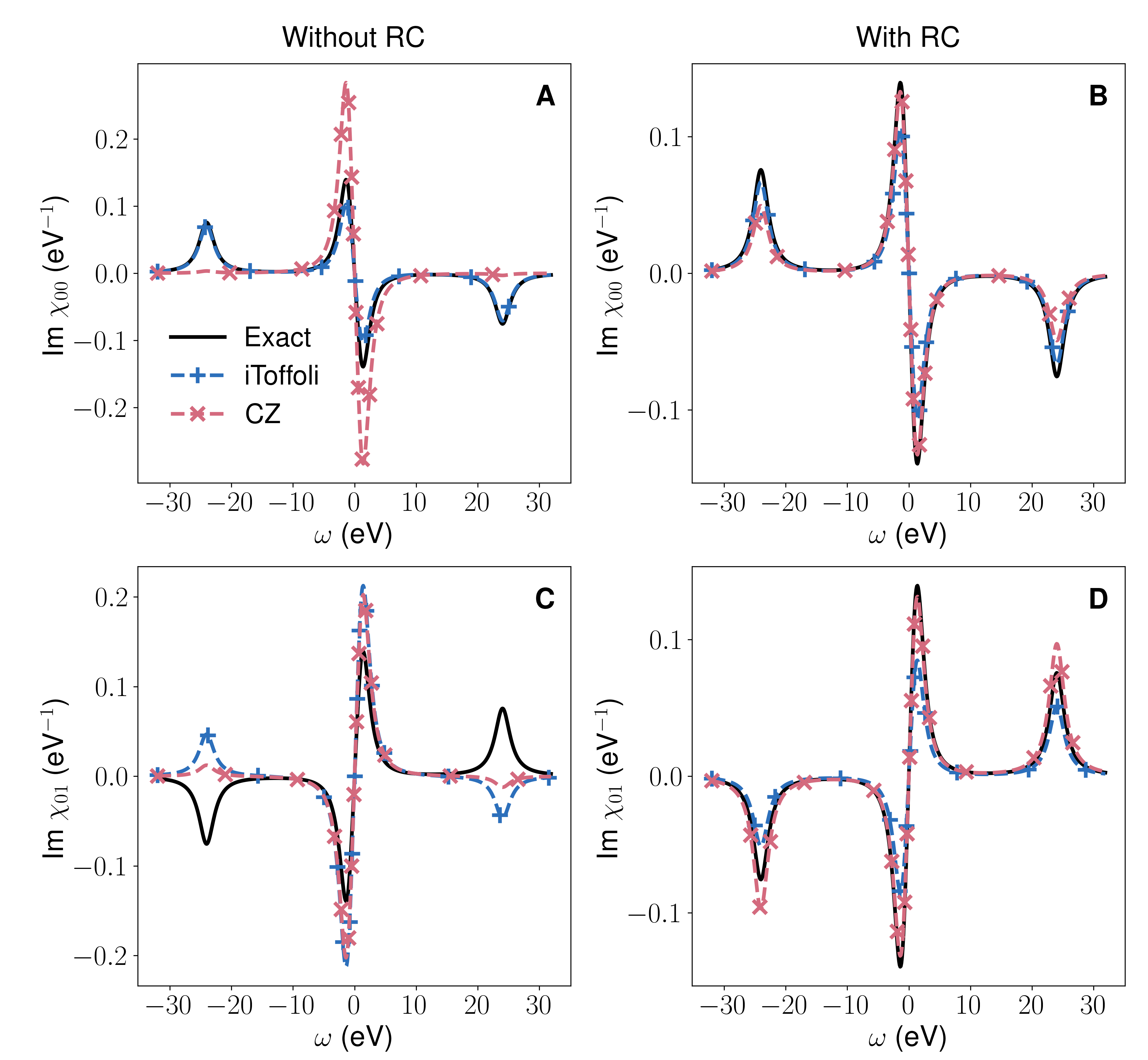
We now show the density-density response functions and of NaH in Fig. 6. Here is obtained from two diagonal circuits and one off-diagonal circuit , while is obtained from four off-diagonal circuits . All experimental results are postprocessed with purification after constraining the ancilla qubits to each bitstring subspace.
Overall, the iToffoli decomposition yields comparable or better results compared to the CZ decomposition. Without RC, the iToffoli decomposition results in visibly better agreement with the exact response functions in Figs. 6 and 6, where the root-mean-squared (RMS) errors between the experimental and exact response functions are 0.0086 eV-1 and 0.0372 eV-1 for the iToffoli decomposition and 0.0387 eV-1 and 0.0278 eV-1 for the CZ decomposition for and , respectively. With RC, the two decompositions exhibit comparable RMS errors, which are 0.0081 eV-1 and 0.0143 eV-1 for the iToffoli decomposition, and are 0.0073 eV-1 and 0.0061 eV-1 for the CZ decomposition for and , respectively, as shown in Figs. 6 and 6.
In both and , RC can lead to substantial improvements in the experimental data for both decompositions, which is reflected in the heights of the symmetric peaks at eV and eV. For without RC and using the CZ decomposition, the peak at eV is twice the height of the exact peak and the peak at eV is not present in the experimental observable in Fig. 6. With RC, both features are present, with the deviations of the peak heights being 34.8% and 4.7%, respectively, as in Fig. 6. For with the iToffoli decomposition, the peak height deviations change from 6.1% and 26.6% without RC in Fig. 6 to 11.8% and 24.0% with RC in Fig. 6. In this case, the results before and after RC are comparable since the experimental observable without RC is already in good agreement with the exact observable. For , we see a more marked improvement due to RC compared to the corresponding results for . Without RC, both iToffoli and CZ decompositions produce the wrong sign on the peak at eV in Fig. 6, but with RC the signs are correctly predicted. The peak height deviations can then be computed as 39.2% and 32.2% for the CZ decompositions and 5.7% and 28.2% for the iToffoli decomposition, as indicated in Fig. 6. The corresponding results of system-qubit state fidelities and density-density response functions for KH are given in Supplementary Sec. V, which follow a similar trend as NaH.
Since the iToffoli gate is non-Clifford, our implementation of RC results in incomplete Pauli twirling compared to applying RC to the CZ-decomposed circuits (see Supplementary Sec. IV). The incompleteness of RC on the iToffoli-decomposed circuits may explain why the two decompositions have similar RMS errors with RC despite the initial advantage for the iToffoli decomposition without RC due to its lower circuit depth.
Discussion
We have carried out an LCU-based algorithm to compute the spectral functions and density-density response functions of diatomic molecules from the transition amplitudes determined on a superconducting quantum processor. Using a native high-fidelity iToffoli gate Kim et al. 2022 has enabled the required circuit depth to be reduced by around a factor of two. These resulting circuits produced better agreement with the exact results compared to the circuits constructed only from CZ, CS, and CS† gates when RC is not employed. We also developed an RC protocol for the non-Clifford iToffoli gate, and have shown that without complete Pauli twirling on the iToffoli gate, the circuits constructed from iToffoli gates gave comparable results as the circuits constructed only from CZ, CS, and CS† gates with RC.
The quality of the computed quantities was greatly improved by the use of several error mitigation techniques. Specifically, our results highlight the significance of RC Wallman and Emerson 2016; Hashim et al. 2021 combined with McWeeny purification McWeeny 1960 for quantum simulation. McWeeny purification has been widely used in quantum chemistry Goedecker 1999 and started to be exploited in quantum computing for constraining the purity of the output state Arute et al. 2020; Ville et al. 2022. Our results have showed that RC or McWeeny purification individually only improves the experimental results to a limited extent, as observed in the change of the average off-diagonal fidelities from 45.8% to 54.2% with only RC, and to 67.4% with only purification in Fig. 5. However, the combination of RC and purification results in a significant improvement in the quality of the results with the system-qubit state fidelities being 96.0% on average. Moreover, previous works applied purification to the whole qubit register, but we have showed here that the purification scheme can be applied when there is purity constraint on a subset of qubits. Additionally, our work is the first to apply RC to the non-Clifford iToffoli gate. As more native non-Clifford two-qubit and multi-qubit gates become available, our findings may guide future application of RC to non-Clifford gates.
Our work is also among the first to demonstrate the practical use of a native multi-qubit gate in quantum simulation via an LCU-based algorithm. LCU as a general algorithmic framework is not limited to determining transition amplitudes in frequency-domain response properties, but has broader applications in areas such as solving linear systems Childs et al. 2017, simulating non-Hermitian dynamics Wen et al. 2019, and preparing quantum Gibbs states Chowdhury and Somma 2017. Besides the LCU algorithm, quantum algorithms such as Shor’s algorithm Shor 1997 and Grover’s search algorithm Grover 1997 can benefit considerably from native three-qubit gates with reduction in circuit depths and gate counts. Quantum algorithm design and implementation thus far have been mostly restricted to single- and two-qubit gates due to their ease of implementation and demonstrated high fidelity. Meanwhile, early implementations of three-qubit gates Mariantoni et al. 2011; Fedorov et al. 2012; Reed et al. 2012 were generally slower and more prone to leakage and decoherence compared to the iToffoli gate employed here due to populating higher levels outside the qubit computational space. However, more recent implementations of three-qubit gates Kim et al. 2022; Hill et al.; Galda et al. have begun to address these challenges yielding fidelities approaching those achieved with two-qubit gates. Further, they have been carried out on quantum devices with tens of qubits, suggesting their utility for larger-scale quantum devices. As such native multi-qubit gates become more prevalent, our work paves the way for using them as native gate components in future quantum algorithm design and implementation.
Methods
Quantum Circuit Construction
The molecular orbitals used in this work are in STO-3G basis with molecular integrals determined from PySCF Sun et al. 2020. We use OpenFermion McClean et al. 2020 to map the second-quantized Hamiltonian to qubit operators. The ground-state preparation gate on the system qubits are determined classically by constructing a unitary that maps the all-zero initial states to the ground state and then decomposed into three CZ gates and single-qubit gates using the decomposition Vatan and Williams 2004. The LCU circuits are then constructed by applying the gates shown in Figs. 1 and 1, where the SWAP gates are decomposed according to the scheme in Ref. Hashim et al. 2022 and the circuits are transpiled by the functions MergeInteractions, MergeSingleQubitGates and DropEmptyMoments in Cirq Developers 2022. The transition amplitudes are then combined with the classically determined ground- and excited-state energies to calculate the spectral functions and response functions (See Supplementary Sec. II).
Quantum Device
The quantum device used in this work is a superconducting quantum processor with eight transmon qubits. The algorithm is performed on a four-qubit subset of the device with linear connectivity. Single-qubit gates are performed with resonant microwave pulses. Multiplexed dispersive readout allows for simultaneous state discrimination on all four qubits. CZ gates between all nearest neighbors are performed according to the method in Ref. Mitchell et al. 2021. The same method allows for a native CS gate on one pair and a native CS† gate on a different pair, according to the requirements of the algorithm. While single-qubit gates are applied simultaneously, microwave crosstalk requires that all two- and three-qubit gates are applied in separate cycles from each other as well as from any single-qubit gates. TrueQ Beale et al. 2020 is used for circuit manipulations in the implementation of RC as well as gate benchmarking. Internal software is used to map the circuits to hardware pulses for implementing the native gate set.
Acknowledgements
The authors acknowledge A. Hashim, E. Younis, Y. Gao, G. Li for helpful discussions. S.-N.S. and A.J.M. are supported by the U.S. Department of Energy under Award No. DE-SC0019374. B.M., L.B.N., and L.C. are supported by the Quantum Testbed Program of the Advanced Scientific Computing Research for Basic Energy Sciences program, Office of Science of the U.S. Department of Energy under Contract No. DE-AC02-05CH11231. Y.K. is supported by the KIST research program under grant No. 2E31531. S.-N.S would like to acknowledge the QISE-NET fellowship for promoting the collaboration between Caltech and UC Berkeley in the field of quantum computing.
Author contributions
S.-N.S. and A.J.M. conceptualized the project. S.-N.S., B.M., and J.M.Koh contributed to the codebase. B.M., L.B.N., L.C., and Y.K. performed the device calibration and hardware runs of the circuits. J.M.Kreikebaum fabricated the device. S.-N.S. and B.M. analyzed the data. All authors contributed to discussion of the manuscript.
References
- Feynman (1982) R. P. Feynman, Simulating physics with computers, Int. J. Theor. Phys. 21, 467 (1982).
- Lloyd (1996) S. Lloyd, Universal Quantum Simulators, Science 273, 1073 (1996).
- Georgescu et al. (2014) I. M. Georgescu, S. Ashhab, and F. Nori, Quantum simulation, Rev. Mod. Phys. 86, 153 (2014).
- Peruzzo et al. (2014) A. Peruzzo, J. McClean, P. Shadbolt, M.-H. Yung, X.-Q. Zhou, P. J. Love, A. Aspuru-Guzik, and J. L. O’Brien, A variational eigenvalue solver on a photonic quantum processor, Nat Commun 5, 4213 (2014).
- O’Malley et al. (2016) P. O’Malley, R. Babbush, I. Kivlichan, J. Romero, J. McClean, R. Barends, J. Kelly, P. Roushan, A. Tranter, N. Ding, B. Campbell, Y. Chen, Z. Chen, B. Chiaro, A. Dunsworth, A. Fowler, E. Jeffrey, E. Lucero, A. Megrant, J. Mutus, M. Neeley, C. Neill, C. Quintana, D. Sank, A. Vainsencher, J. Wenner, T. White, P. Coveney, P. Love, H. Neven, A. Aspuru-Guzik, and J. Martinis, Scalable Quantum Simulation of Molecular Energies, Physical Review X 6, 031007 (2016).
- Kandala et al. (2017) A. Kandala, A. Mezzacapo, K. Temme, M. Takita, M. Brink, J. M. Chow, and J. M. Gambetta, Hardware-efficient variational quantum eigensolver for small molecules and quantum magnets, Nature 549, 242 (2017).
- Colless et al. (2018) J. Colless, V. Ramasesh, D. Dahlen, M. Blok, M. Kimchi-Schwartz, J. McClean, J. Carter, W. de Jong, and I. Siddiqi, Computation of Molecular Spectra on a Quantum Processor with an Error-Resilient Algorithm, Physical Review X 8, 011021 (2018).
- Barends et al. (2015) R. Barends, L. Lamata, J. Kelly, L. García-Álvarez, A. G. Fowler, A. Megrant, E. Jeffrey, T. C. White, D. Sank, J. Y. Mutus, B. Campbell, Y. Chen, Z. Chen, B. Chiaro, A. Dunsworth, I.-C. Hoi, C. Neill, P. J. J. O’Malley, C. Quintana, P. Roushan, A. Vainsencher, J. Wenner, E. Solano, and J. M. Martinis, Digital quantum simulation of fermionic models with a superconducting circuit, Nat Commun 6, 7654 (2015).
- Arute et al. (2020) F. Arute, K. Arya, R. Babbush, D. Bacon, J. C. Bardin, R. Barends, S. Boixo, M. Broughton, B. B. Buckley, D. A. Buell, B. Burkett, N. Bushnell, Y. Chen, Z. Chen, B. Chiaro, R. Collins, W. Courtney, S. Demura, A. Dunsworth, E. Farhi, A. Fowler, B. Foxen, C. Gidney, M. Giustina, R. Graff, S. Habegger, M. P. Harrigan, A. Ho, S. Hong, T. Huang, W. J. Huggins, L. Ioffe, S. V. Isakov, E. Jeffrey, Z. Jiang, C. Jones, D. Kafri, K. Kechedzhi, J. Kelly, S. Kim, P. V. Klimov, A. Korotkov, F. Kostritsa, D. Landhuis, P. Laptev, M. Lindmark, E. Lucero, O. Martin, J. M. Martinis, J. R. McClean, M. McEwen, A. Megrant, X. Mi, M. Mohseni, W. Mruczkiewicz, J. Mutus, O. Naaman, M. Neeley, C. Neill, H. Neven, M. Y. Niu, T. E. O’Brien, E. Ostby, A. Petukhov, H. Putterman, C. Quintana, P. Roushan, N. C. Rubin, D. Sank, K. J. Satzinger, V. Smelyanskiy, D. Strain, K. J. Sung, M. Szalay, T. Y. Takeshita, A. Vainsencher, T. White, N. Wiebe, Z. J. Yao, P. Yeh, and A. Zalcman, Hartree-Fock on a superconducting qubit quantum computer, Science 369, 1084 (2020).
- Tazhigulov et al. (2022) R. N. Tazhigulov, S.-N. Sun, R. Haghshenas, H. Zhai, A. T. Tan, N. C. Rubin, R. Babbush, A. J. Minnich, and G. K.-L. Chan, Simulating Models of Challenging Correlated Molecules and Materials on the Sycamore Quantum Processor, PRX Quantum 3, 040318 (2022).
- Stanisic et al. (2022) S. Stanisic, J. L. Bosse, F. M. Gambetta, R. A. Santos, W. Mruczkiewicz, T. E. O’Brien, E. Ostby, and A. Montanaro, Observing ground-state properties of the Fermi-Hubbard model using a scalable algorithm on a quantum computer, Nat Commun 13, 5743 (2022).
- Motta et al. (2019) M. Motta, C. Sun, A. T. K. Tan, M. J. O’Rourke, E. Ye, A. J. Minnich, F. G. S. L. Brandão, and G. K.-L. Chan, Determining eigenstates and thermal states on a quantum computer using quantum imaginary time evolution, Nat. Phys. 10.1038/s41567-019-0704-4 (2019).
- Francis et al. (2021) A. Francis, D. Zhu, C. Huerta Alderete, S. Johri, X. Xiao, J. K. Freericks, C. Monroe, N. M. Linke, and A. F. Kemper, Many-body thermodynamics on quantum computers via partition function zeros, Sci. Adv. 7, eabf2447 (2021).
- Satzinger et al. (2021) K. J. Satzinger, Y.-J. Liu, A. Smith, C. Knapp, M. Newman, C. Jones, Z. Chen, C. Quintana, X. Mi, A. Dunsworth, C. Gidney, I. Aleiner, F. Arute, K. Arya, J. Atalaya, R. Babbush, J. C. Bardin, R. Barends, J. Basso, A. Bengtsson, A. Bilmes, M. Broughton, B. B. Buckley, D. A. Buell, B. Burkett, N. Bushnell, B. Chiaro, R. Collins, W. Courtney, S. Demura, A. R. Derk, D. Eppens, C. Erickson, L. Faoro, E. Farhi, A. G. Fowler, B. Foxen, M. Giustina, A. Greene, J. A. Gross, M. P. Harrigan, S. D. Harrington, J. Hilton, S. Hong, T. Huang, W. J. Huggins, L. B. Ioffe, S. V. Isakov, E. Jeffrey, Z. Jiang, D. Kafri, K. Kechedzhi, T. Khattar, S. Kim, P. V. Klimov, A. N. Korotkov, F. Kostritsa, D. Landhuis, P. Laptev, A. Locharla, E. Lucero, O. Martin, J. R. McClean, M. McEwen, K. C. Miao, M. Mohseni, S. Montazeri, W. Mruczkiewicz, J. Mutus, O. Naaman, M. Neeley, C. Neill, M. Y. Niu, T. E. O’Brien, A. Opremcak, B. Pató, A. Petukhov, N. C. Rubin, D. Sank, V. Shvarts, D. Strain, M. Szalay, B. Villalonga, T. C. White, Z. Yao, P. Yeh, J. Yoo, A. Zalcman, H. Neven, S. Boixo, A. Megrant, Y. Chen, J. Kelly, V. Smelyanskiy, A. Kitaev, M. Knap, F. Pollmann, and P. Roushan, Realizing topologically ordered states on a quantum processor, Science 374, 1237 (2021).
- Tan et al. (2021) A. T. K. Tan, S.-N. Sun, R. N. Tazhigulov, G. K.-L. Chan, and A. J. Minnich, Realizing symmetry-protected topological phases in a spin-1/2 chain with next-nearest neighbor hopping on superconducting qubits (2021), arXiv:2112.10333 [quant-ph].
- mi_ (2022) Time-crystalline eigenstate order on a quantum processor, Nature 601, 531 (2022).
- Karamlou et al. (2022) A. H. Karamlou, J. Braumüller, Y. Yanay, A. Di Paolo, P. M. Harrington, B. Kannan, D. Kim, M. Kjaergaard, A. Melville, S. Muschinske, B. M. Niedzielski, A. Vepsäläinen, R. Winik, J. L. Yoder, M. Schwartz, C. Tahan, T. P. Orlando, S. Gustavsson, and W. D. Oliver, Quantum transport and localization in 1d and 2d tight-binding lattices, npj Quantum Inf 8, 35 (2022).
- Niu et al. (2022) D. Niu, R. Haghshenas, Y. Zhang, M. Foss-Feig, G. K.-L. Chan, and A. C. Potter, Holographic Simulation of Correlated Electrons on a Trapped-Ion Quantum Processor, PRX Quantum 3, 030317 (2022).
- Chertkov et al. (2022) E. Chertkov, J. Bohnet, D. Francois, J. Gaebler, D. Gresh, A. Hankin, K. Lee, D. Hayes, B. Neyenhuis, R. Stutz, A. C. Potter, and M. Foss-Feig, Holographic dynamics simulations with a trapped-ion quantum computer, Nat. Phys. 18, 1074 (2022).
- Gibbs et al. (2022) J. Gibbs, K. Gili, Z. Holmes, B. Commeau, A. Arrasmith, L. Cincio, P. J. Coles, and A. Sornborger, Long-time simulations for fixed input states on quantum hardware, npj Quantum Inf 8, 135 (2022).
- Arute et al. (2019) F. Arute, K. Arya, R. Babbush, D. Bacon, J. C. Bardin, R. Barends, R. Biswas, S. Boixo, F. G. S. L. Brandao, D. A. Buell, B. Burkett, Y. Chen, Z. Chen, B. Chiaro, R. Collins, W. Courtney, A. Dunsworth, E. Farhi, B. Foxen, A. Fowler, C. Gidney, M. Giustina, R. Graff, K. Guerin, S. Habegger, M. P. Harrigan, M. J. Hartmann, A. Ho, M. Hoffmann, T. Huang, T. S. Humble, S. V. Isakov, E. Jeffrey, Z. Jiang, D. Kafri, K. Kechedzhi, J. Kelly, P. V. Klimov, S. Knysh, A. Korotkov, F. Kostritsa, D. Landhuis, M. Lindmark, E. Lucero, D. Lyakh, S. Mandrà, J. R. McClean, M. McEwen, A. Megrant, X. Mi, K. Michielsen, M. Mohseni, J. Mutus, O. Naaman, M. Neeley, C. Neill, M. Y. Niu, E. Ostby, A. Petukhov, J. C. Platt, C. Quintana, E. G. Rieffel, P. Roushan, N. C. Rubin, D. Sank, K. J. Satzinger, V. Smelyanskiy, K. J. Sung, M. D. Trevithick, A. Vainsencher, B. Villalonga, T. White, Z. J. Yao, P. Yeh, A. Zalcman, H. Neven, and J. M. Martinis, Quantum supremacy using a programmable superconducting processor, Nature 574, 505 (2019).
- Wu et al. (2021) Y. Wu, W.-S. Bao, S. Cao, F. Chen, M.-C. Chen, X. Chen, T.-H. Chung, H. Deng, Y. Du, D. Fan, M. Gong, C. Guo, C. Guo, S. Guo, L. Han, L. Hong, H.-L. Huang, Y.-H. Huo, L. Li, N. Li, S. Li, Y. Li, F. Liang, C. Lin, J. Lin, H. Qian, D. Qiao, H. Rong, H. Su, L. Sun, L. Wang, S. Wang, D. Wu, Y. Xu, K. Yan, W. Yang, Y. Yang, Y. Ye, J. Yin, C. Ying, J. Yu, C. Zha, C. Zhang, H. Zhang, K. Zhang, Y. Zhang, H. Zhao, Y. Zhao, L. Zhou, Q. Zhu, C.-Y. Lu, C.-Z. Peng, X. Zhu, and J.-W. Pan, Strong Quantum Computational Advantage Using a Superconducting Quantum Processor, Phys. Rev. Lett. 127, 180501 (2021).
- Daley et al. (2022) A. J. Daley, I. Bloch, C. Kokail, S. Flannigan, N. Pearson, M. Troyer, and P. Zoller, Practical quantum advantage in quantum simulation, Nature 607, 667 (2022).
- Cao et al. (2019) Y. Cao, J. Romero, J. P. Olson, M. Degroote, P. D. Johnson, M. Kieferová, I. D. Kivlichan, T. Menke, B. Peropadre, N. P. D. Sawaya, S. Sim, L. Veis, and A. Aspuru-Guzik, Quantum Chemistry in the Age of Quantum Computing, Chem. Rev. 119, 10856 (2019).
- (25) S. McArdle, S. Endo, A. Aspuru-Guzik, S. C. Benjamin, and X. Yuan, Quantum computational chemistry, Rev. Mod. Phys. 92, 015003.
- Bauer et al. (2020) B. Bauer, S. Bravyi, M. Motta, and G. K.-L. Chan, Quantum Algorithms for Quantum Chemistry and Quantum Materials Science, Chem. Rev. 120, 12685 (2020).
- von Nissen et al. (1984) W. von Nissen, J. Schirmer, and L. S. Cederbaum, Computational Methods for the One-Particle Green’s Function, Computer Physics Reports 1, 57 (1984).
- Ullrich (2019) C. A. Ullrich, Time-Dependent Density-Functional Theory : Concepts and Applications, Oxford graduate texts (OXFORD UNIV Press, Place of publication not identified, 2019).
- Damascelli et al. (2003) A. Damascelli, Z. Hussain, and Z.-X. Shen, Angle-resolved photoemission studies of the cuprate superconductors, Rev. Mod. Phys. 75, 473 (2003).
- Chiesa et al. (2019) A. Chiesa, F. Tacchino, M. Grossi, P. Santini, I. Tavernelli, D. Gerace, and S. Carretta, Quantum hardware simulating four-dimensional inelastic neutron scattering, Nat. Phys. 15, 455 (2019).
- Francis et al. (2020) A. Francis, J. K. Freericks, and A. F. Kemper, Quantum computation of magnon spectra, Phys. Rev. B 101, 014411 (2020).
- Sun et al. (2021) S.-N. Sun, M. Motta, R. N. Tazhigulov, A. T. Tan, G. K.-L. Chan, and A. J. Minnich, Quantum Computation of Finite-Temperature Static and Dynamical Properties of Spin Systems Using Quantum Imaginary Time Evolution, PRX Quantum 2, 010317 (2021).
- McClean et al. (2017) J. R. McClean, M. E. Kimchi-Schwartz, J. Carter, and W. A. de Jong, Hybrid quantum-classical hierarchy for mitigation of decoherence and determination of excited states, Phys. Rev. A 95, 042308 (2017).
- Nakanishi et al. (2019) K. M. Nakanishi, K. Mitarai, and K. Fujii, Subspace-search variational quantum eigensolver for excited states, Phys. Rev. Research 1, 033062 (2019).
- Parrish et al. (2019) R. M. Parrish, E. G. Hohenstein, P. L. McMahon, and T. J. Martínez, Quantum Computation of Electronic Transitions Using a Variational Quantum Eigensolver, Phys. Rev. Lett. 122, 230401 (2019).
- Higgott et al. (2019) O. Higgott, D. Wang, and S. Brierley, Variational Quantum Computation of Excited States, Quantum 3, 156 (2019).
- Jones et al. (2019) T. Jones, S. Endo, S. McArdle, X. Yuan, and S. C. Benjamin, Variational quantum algorithms for discovering Hamiltonian spectra, Phys. Rev. A 99, 062304 (2019).
- Endo et al. (2020) S. Endo, I. Kurata, and Y. O. Nakagawa, Calculation of the green’s function on near-term quantum computers, Phys. Rev. Research 2, 033281 (2020).
- (39) H. Chen, M. Nusspickel, J. Tilly, and G. H. Booth, A variational quantum eigensolver for dynamic correlation functions, arXiv: 2105.01703 .
- Jamet et al. (2022) F. Jamet, A. Agarwal, and I. Rungger, Quantum subspace expansion algorithm for Green’s functions (2022), arXiv:2205.00094 [quant-ph].
- Cai et al. (2020) X. Cai, W.-H. Fang, H. Fan, and Z. Li, Quantum computation of molecular response properties, Physical Review Research 2, 033324 (2020).
- Kosugi and Matsushita (2020a) T. Kosugi and Y.-i. Matsushita, Construction of Green’s functions on a quantum computer: Quasiparticle spectra of molecules, Phys. Rev. A 101, 012330 (2020a).
- Kosugi and Matsushita (2020b) T. Kosugi and Y.-i. Matsushita, Linear-response functions of molecules on a quantum computer: Charge and spin responses and optical absorption, Phys. Rev. Research 2, 033043 (2020b).
- (44) A. M. Childs and N. Wiebe, Hamiltonian simulation using linear combinations of unitary operations, Quantum Information and Computation 12, 10.26421/QIC12.11-12, 1202.5822 .
- Kim et al. (2022) Y. Kim, A. Morvan, L. B. Nguyen, R. K. Naik, C. Jünger, L. Chen, J. M. Kreikebaum, D. I. Santiago, and I. Siddiqi, High-fidelity three-qubit iToffoli gate for fixed-frequency superconducting qubits, Nat. Phys. 10.1038/s41567-022-01590-3 (2022).
- Wallman and Emerson (2016) J. J. Wallman and J. Emerson, Noise tailoring for scalable quantum computation via randomized compiling, Phys. Rev. A 94, 052325 (2016).
- Hashim et al. (2021) A. Hashim, R. K. Naik, A. Morvan, J.-L. Ville, B. Mitchell, J. M. Kreikebaum, M. Davis, E. Smith, C. Iancu, K. P. O’Brien, I. Hincks, J. J. Wallman, J. Emerson, and I. Siddiqi, Randomized Compiling for Scalable Quantum Computing on a Noisy Superconducting Quantum Processor, Phys. Rev. X 11, 041039 (2021).
- McWeeny (1960) R. McWeeny, Some Recent Advances in Density Matrix Theory, Rev. Mod. Phys. 32, 335 (1960).
- Yeter‐Aydeniz et al. (2021) K. Yeter‐Aydeniz, B. T. Gard, J. Jakowski, S. Majumder, G. S. Barron, G. Siopsis, T. S. Humble, and R. C. Pooser, Benchmarking Quantum Chemistry Computations with Variational, Imaginary Time Evolution, and Krylov Space Solver Algorithms, Adv Quantum Tech 4, 2100012 (2021).
- Jordan and Wigner (1928) P. Jordan and E. Wigner, Über das Paulische Äquivalenzverbot, Z. Physik 47, 631 (1928).
- (51) S. Bravyi, J. M. Gambetta, A. Mezzacapo, and K. Temme, Tapering off qubits to simulate fermionic Hamiltonians, arXiv: 1701.08213 .
- Christandl and Renner (2012) M. Christandl and R. Renner, Reliable Quantum State Tomography, Phys. Rev. Lett. 109, 120403 (2012).
- Whitfield et al. (2011) J. D. Whitfield, J. Biamonte, and A. Aspuru-Guzik, Simulation of electronic structure Hamiltonians using quantum computers, Molecular Physics 109, 735 (2011).
- Hashim et al. (2022) A. Hashim, R. Rines, V. Omole, R. K. Naik, J. M. Kreikebaum, D. I. Santiago, F. T. Chong, I. Siddiqi, and P. Gokhale, Optimized swap networks with equivalent circuit averaging for qaoa, Phys. Rev. Research 4, 033028 (2022).
- Younis et al. (2021) E. Younis, C. C. Iancu, W. Lavrijsen, M. Davis, E. Smith, and USDOE, Berkeley quantum synthesis toolkit (bqskit) v1 (2021).
- Shende and Markov (2009) V. Shende and I. Markov, On the CNOT -cost of TOFFOLI gates, QIC 9, 461 (2009).
- Goedecker (1999) S. Goedecker, Linear scaling electronic structure methods, Rev. Mod. Phys. 71, 1085 (1999).
- Ville et al. (2022) J.-L. Ville, A. Morvan, A. Hashim, R. K. Naik, M. Lu, B. Mitchell, J.-M. Kreikebaum, K. P. O’Brien, J. J. Wallman, I. Hincks, J. Emerson, E. Smith, E. Younis, C. Iancu, D. I. Santiago, and I. Siddiqi, Leveraging randomized compiling for the quantum imaginary-time-evolution algorithm, Phys. Rev. Research 4, 033140 (2022).
- Childs et al. (2017) A. M. Childs, R. Kothari, and R. D. Somma, Quantum algorithm for systems of linear equations with exponentially improved dependence on precision, SIAM Journal on Computing 46, 1920 (2017).
- Wen et al. (2019) J. Wen, C. Zheng, X. Kong, S. Wei, T. Xin, and G. Long, Experimental demonstration of a digital quantum simulation of a general PT -symmetric system, Phys. Rev. A 99, 062122 (2019).
- Chowdhury and Somma (2017) A. N. Chowdhury and R. D. Somma, Quantum algorithms for Gibbs sampling and hitting-time estimation, Quantum Information & Computation 17, 41 (2017).
- Shor (1997) P. W. Shor, Polynomial-Time Algorithms for Prime Factorization and Discrete Logarithms on a Quantum Computer, SIAM Journal on Computing 26, 1484 (1997).
- Grover (1997) L. K. Grover, Quantum Mechanics Helps in Searching for a Needle in a Haystack, Phys. Rev. Lett. 79, 325 (1997).
- Mariantoni et al. (2011) M. Mariantoni, H. Wang, T. Yamamoto, M. Neeley, R. C. Bialczak, Y. Chen, M. Lenander, E. Lucero, A. D. O’Connell, D. Sank, M. Weides, J. Wenner, Y. Yin, J. Zhao, A. N. Korotkov, A. N. Cleland, and J. M. Martinis, Implementing the Quantum von Neumann Architecture with Superconducting Circuits, Science 334, 61 (2011).
- Fedorov et al. (2012) A. Fedorov, L. Steffen, M. Baur, M. P. da Silva, and A. Wallraff, Implementation of a Toffoli gate with superconducting circuits, Nature 481, 170 (2012).
- Reed et al. (2012) M. D. Reed, L. DiCarlo, S. E. Nigg, L. Sun, L. Frunzio, S. M. Girvin, and R. J. Schoelkopf, Realization of three-qubit quantum error correction with superconducting circuits, Nature 482, 382 (2012).
- (67) A. D. Hill, M. J. Hodson, N. Didier, and M. J. Reagor, Realization of arbitrary doubly-controlled quantum phase gates, arXiv:2108.01652 .
- (68) A. Galda, M. Cubeddu, N. Kanazawa, P. Narang, and N. Earnest-Noble, Implementing a Ternary Decomposition of the Toffoli Gate on Fixed-Frequency Transmon Qutrits, arXiv:2109.00558 .
- Sun et al. (2020) Q. Sun, X. Zhang, S. Banerjee, P. Bao, M. Barbry, N. S. Blunt, N. A. Bogdanov, G. H. Booth, J. Chen, Z.-H. Cui, J. J. Eriksen, Y. Gao, S. Guo, J. Hermann, M. R. Hermes, K. Koh, P. Koval, S. Lehtola, Z. Li, J. Liu, N. Mardirossian, J. D. McClain, M. Motta, B. Mussard, H. Q. Pham, A. Pulkin, W. Purwanto, P. J. Robinson, E. Ronca, E. R. Sayfutyarova, M. Scheurer, H. F. Schurkus, J. E. T. Smith, C. Sun, S.-N. Sun, S. Upadhyay, L. K. Wagner, X. Wang, A. White, J. D. Whitfield, M. J. Williamson, S. Wouters, J. Yang, J. M. Yu, T. Zhu, T. C. Berkelbach, S. Sharma, A. Y. Sokolov, and G. K.-L. Chan, Recent developments in the PySCF program package, J. Chem. Phys. 153, 024109 (2020).
- McClean et al. (2020) J. R. McClean, N. C. Rubin, K. J. Sung, I. D. Kivlichan, X. Bonet-Monroig, Y. Cao, C. Dai, E. S. Fried, C. Gidney, B. Gimby, P. Gokhale, T. Häner, T. Hardikar, V. Havlíček, O. Higgott, C. Huang, J. Izaac, Z. Jiang, X. Liu, S. McArdle, M. Neeley, T. O’Brien, B. O’Gorman, I. Ozfidan, M. D. Radin, J. Romero, N. P. D. Sawaya, B. Senjean, K. Setia, S. Sim, D. S. Steiger, M. Steudtner, Q. Sun, W. Sun, D. Wang, F. Zhang, and R. Babbush, OpenFermion: the electronic structure package for quantum computers, Quantum Sci. Technol. 5, 034014 (2020).
- Vatan and Williams (2004) F. Vatan and C. Williams, Optimal quantum circuits for general two-qubit gates, Phys. Rev. A 69, 032315 (2004).
- Developers (2022) C. Developers, Cirq (2022), See full list of authors on Github: https://github .com/quantumlib/Cirq/graphs/contributors.
- Mitchell et al. (2021) B. K. Mitchell, R. K. Naik, A. Morvan, A. Hashim, J. M. Kreikebaum, B. Marinelli, W. Lavrijsen, K. Nowrouzi, D. I. Santiago, and I. Siddiqi, Hardware-efficient microwave-activated tunable coupling between superconducting qubits, Phys. Rev. Lett. 127, 200502 (2021).
- Beale et al. (2020) S. J. Beale, A. Carignan-Dugas, D. Dahlen, J. Emerson, I. Hincks, P. Iyer, A. Jain, D. Hufnagel, E. Ospadov, J. Saunders, A. Stasiuk, J. J. Wallman, and A. Winick, True-q (2020).
- Erhard et al. (2019) A. Erhard, J. J. Wallman, L. Postler, M. Meth, R. Stricker, E. A. Martinez, P. Schindler, T. Monz, J. Emerson, and R. Blatt, Characterizing large-scale quantum computers via cycle benchmarking, Nature Comms. 10, 5347 (2019).
Supplemental Materials: Quantum Computation of Frequency-Domain Molecular Response Properties Using a Three-Qubit iToffoli Gate
I symmetry transformations on operators and qubit states
In this section, we describe the symmetry transformations applied to the qubit operators and ancilla qubit subspaces in the linear combination of unitaries (LCU) algorithm. This transformation converts the four-qubit operators and qubit subspaces into two-qubit ones, which are used in constructing the circuits for hardware runs.
There are four spin orbitals in the diatomic molecules we study in this work. We order them as from left to right, corresponding to the qubit indices 0, 1, 2, 3, in the Pauli strings and qubit state bitstrings. The HOMO-LUMO molecular Hamiltonians of NaH and KH have the same number of up-spin and down-spin electrons. After Jordan-Wigner transformation, the parity of up-spin and down-spin electrons correspond to the qubit operators and , which are symmetries of the Hamiltonian. The mean-field ground state has the expectation values , as does the exact ground state .
We can define three types of states in our calculation based on symmetries: the “up-spin” states are the states that have symmetries , which are obtained by applying or on the ground state; the “down-spin” states are the states that have symmetries , which are obtained by applying or on the ground state; the “spin-balanced” states are the states that have the symmetries , which are obtained by applying the number operators on the ground state and have the same symmetries as the ground state. Note that the up-spin and down-spin states here are defined from the expectation values of the symmetry operators but do not correspond to spin- components of the corresponding molecular states. For example, the qubit computational state represents the molecular state with a single electron in the orbital, which has total spin- expectation value of , but in our definition it is classified as an up-spin state.
For each type of state, we aim to find a transformation that generates the minimum number of gates in the circuits that apply the creation or annihilation operators or the number operators . Recall from the main text that in the Jordan-Wigner transformation, the creation or annihilation operators have the decomposition , where and are the Jordan-Wigner transformed Pauli and operators on orbital with spin , and the number operators have the decomposition . The transition amplitudes under the transformation can be expressed as
| (1) | ||||
| (2) |
where the transformed bra state, ket state and operator are grouped in brackets at the end of each equation. On the up-spin states, we use the transformation ; on the down-spin states, we use the transformation , followed by multiplying all the operators by ; on the spin-balanced states, we use the transformation . After the transformation, the first two qubits on the operators and the states are then truncated.
As an example, consider the transformation of the Pauli string . After we apply the transformation CNOT(3, 1)CNOT(2, 0), the operator becomes . To truncate qubit 0 and qubit 1, we need to find the constant factor after the transformed Pauli string acts on the first two qubits of the ground state. The constant factor for is , where are the bit values on the first two qubits of the transformed up-spin states and are the bit values on the first two qubits of the transformed ground state . The factor of is then combined with the rest of the Pauli string to give the final truncated form of the Pauli string . The Pauli strings and qubit state bitstrings before and after the symmetry transformations and truncations are given in Table 1.
| Transformed Pauli string symbol | Original Pauli strings | Transformed Pauli strings | Original qubit state bitstrings | Transformed qubit state bitstrings | |
|---|---|---|---|---|---|
| Up-spin | -electron: | -electron: | |||
| 1110, 1011, | 10, 11, | ||||
| -electron: | -electron: | ||||
| 0100, 0001. | 00, 01. | ||||
| Down-spin | -electron: | -electron: | |||
| 1101, 0111. | 10, 11. | ||||
| -electron: | -electron: | ||||
| 1000, 0010 | 00, 01. | ||||
| Spin-balanced | 1100, | 00, | |||
| 1001, | 01, | ||||
| 0110, | 10, | ||||
| 0011. | 11. |
II Calculation of Transition Amplitudes
In this section, we give the equations used to calculate transition amplitudes in the spectral function and density-density response function from quantities measured on hardware. We use the same notation as in the main text, where is the -electron ground state, are the -electron states, and are the -electron excited states. The transition amplitudes follow the same notation as in Ref. Kosugi and Matsushita 2020a, where the transition amplitudes from the ground state to the -electron eigenstates in the calculation of spectral functions are
| (3) | ||||
| (4) |
The spectral function only requires the diagonal transition amplitudes. Theoretically the (unnormalized) states after restraining the ancilla to the 0 or 1 state is . Let the tomographed density matrices corresponding to these states be . The diagonal transition amplitudes are calculated as the overlap between the -electron eigenstates and the tomographed density matrices :
| (5) | ||||
| (6) |
Similarly, in the calculation of density-density response functions, we follow the notation in Ref. Kosugi and Matsushita 2020b and define the transition amplitudes from the ground state to -electron eigenstates as
| (7) |
In the diagonal circuits, theoretically the (unnormalized) state after restraining the ancilla qubit to the 1 state is . Let the corresponding tomographed density matrix obtained from experiments be . The diagonal transition amplitudes are calculated by taking the overlap of the -electron eigenstates and the tomographed density matrix :
| (8) |
In the off-diagonal circuits, theoretically the (unnormalized) states after restraining the ancilla qubits to or states are . Let the corresponding tomographed states obtained from experiments be . The intermediate transition amplitudes obtained directly from are defined as
| (9) |
from which the off-diagonal transition amplitude is determined by Eq. 25 in Ref. Kosugi and Matsushita 2020b (or equivalently Eq. 18 in Ref. Kosugi and Matsushita 2020a) as
| (10) |
III Calibration of the iToffoli Gate

This work employs the recently developed C--C iToffoli gate Kim et al. 2022. In this section we outline the procedure for eliminating spectator errors during the gate application. Since the gate acts on a three qubit subset of the full four qubit subsystem we need to understand and correct the spectator error on the fourth qubit. For concreteness we label qubits for with the iToffoli acting on , , and with as spectator and denote states in the form . We run a simple circuit where we prepare the system in either or (where ) and apply the iToffoli gate in a Ramsey-like sequence to determine the rotation on conditional on the state of its nearest neighbor, (see Fig. S1 for circuit diagram). We observe an unwanted conditional phase interaction between and with conditional phase, (see Fig. S1). This interaction results from the conditional Stark shift between and when a strong off resonant drive is applied to at the frequency of to implement the iToffoli gate Mitchell et al. 2021. We can use the same effect to undo the conditional phase by applying simultaneous off-resonant drives to and for a period following the iToffoli drive sequence. The full pulse sequence and characterization of the residual conditional rotation with the cancellation applied are shown in Fig. S1-S1. We benchmark the resulting gate implementation using Cycle Benchmarking Erhard et al. 2019. With this correction, we measure a gate fidelity of when isolated to the cycle involving qubits that participate in the iToffoli gate, and a small reduction to when including the idling spectator qubit.
IV Randomized Compiling for Non-Clifford Gates
In this section we outline a modified version of randomized compiling (RC) Hashim et al. 2021; Wallman and Emerson 2016 that is applied to the circuits used to compute the observables in the main text. RC is expected to mitigate errors and improve algorithm performance. A broad native entangling gate set is used, consisting of both Clifford gates (CZ) and non-Clifford gates (CS†, CS, iToffoli). RC is typically used with hard cycles of -qubit Cliffords in which case the twirling group is chosen to be the group of tensor products of single qubit Paulis. By the definition of Clifford gates, for any Clifford and twirling gate there is some such that . RC applied to hard cycles of Clifford gates, then proceeds by choosing some for each hard cycle , letting and compiling the single qubit Paulis and into the easy cycles of single qubit gates before and after, respectively, the Clifford cycle .
In order to generalize the method to the non-Clifford gates employed in this work we first find the subsets for where for all there is some such that . Then RC proceeds in the same way as above except the twirling gates for hard cycles consisting of gate are simply chosen from the subset of Pauli strings that stabilize gate . Both the CS and CS† are stabilized by 4 of the possible 16 two-qubit Pauli strings and the iToffoli is stabilized by 8 of the possible 64 three-qubit Pauli strings. For all these non-Clifford gates the twirling and inversion gate are the same, . Results “with RC” in the main text involve averaging the experimental bitstring output distributions over 100 equivalent circuit randomizations generated according to the process outlined here, with each circuit measured for 500 shots. These are compared to results “without RC” in which the bare circuit is measured for 50000 shots (such that the total number of shots is maintained between the two implementations).
All error processes can be described by a superoperator acting on the system density matrix . Written in the -qubit Pauli basis this error process matrix is referred to as a Pauli Transfer Matrix (PTM) with diagonal elements giving Pauli fidelities and off-diagonal elements characterizing the unitary (coherent) and non-unitary (incoherent) errors. As discussed in Hashim et al. 2021; Wallman and Emerson 2016, applying RC tailors coherent errors into stochastic Pauli noise, which suppresses the off-diagonal elements of the PTM. This holds for the PTM describing errors during the CZ cycles, since these undergo perfect Pauli twirling (in the limit of infinite randomizations). However, in the case of the non-Clifford gate cycles, the twirling is imperfect (since we only twirl over a subset of the -qubit Pauli strings). As a result, some, but not all, of the off-diagonal elements in the corresponding PTMs are suppressed. In other words, not all coherent errors are tailored to stochastic Pauli noise. This imperfect noise tailoring is the main limitation of our approach to generalizing RC to non-Clifford gates.
We observe a small improvement in the raw state fidelities when using RC but a much larger improvement in the purified state fidelities with respect to the results without RC. The small improvement in the raw fidelities can be explained by the suppression of off-diagonal components of the error process matrix when using RC which lowers the overall error rate slightly. The larger improvement with purification is explained by the fact that RC tailors coherent errors into Stochastic Pauli errors. If the rates of various stochastic Pauli errors are similar, the errors are largely depolarizing and can be corrected by the purification procedure, yielding the high fidelities in Fig. 5. The deviation of the noise from purely depolarizing is responsible (along with the finite number of randomizations) for the remaining infidelity after RC and purification are applied. Conversely, without RC a larger fraction of the error is a coherent over/under rotation of the two-qubit Bloch vector which cannot be corrected by purification.
V Additional Data for KH


This section presents the system-qubit state fidelities and density-density response functions of the KH molecule. Figure S2 shows the system-qubit state fidelities in the response function calculations of KH. In the case of RC without purification, the average off-diagonal fidelity improved from 49.2% in Fig. S2 to 61.3% in Fig. S2, whereas the average diagonal fidelity slightly decreased from 91.5% in Fig. S2 to 90.5% in Fig. S2. Purification without RC shows a unified improvement across both diagonal and off-diagonal fidelities, which change to 97.1% and 66.9% from 49.2% and 91.5% respectively from Fig. S2 to Fig. S2. The most significant improvement again comes from applying both purification and RC, with the average diagonal fidelity 99.8% and average off-diagonal fidelity 95.9% in Fig. S2.
Figure S3 shows the density-density response functions of KH with all data postprocessed with McWeeny purification. As compared to the case for NaH, the results without RC only fail to reproduce the peaks or produce peaks with the wrong signs in Fig. S3, but reproduce all the peaks in Figs. S3 and S3. As for comparison between the iToffoli decomposition and CZ decomposition, the root-mean-squared deviations without RC are 0.0108 eV-1 for iToffoli and 0.0316 eV-1 for CZ in Fig. S3, while the deviations are 0.1007 eV-1 for iToffoli and 0.0824 eV-1 for CZ in Fig. S3. With RC, the root-mean-squared deviations are 0.0148 eV-1 for iToffoli and 0.0225 eV-1 for CZ in Fig. S3, and 0.0386 eV-1 for iToffoli and 0.0064 eV-1 for CZ in Fig. S3. In all cases with or without RC, the two decompositions show comparable results in the response functions.