06CCS: Computing methodologies Machine learningCCS: Mathematics of computing Probability and statistics

Benedikt Höltgen email: benedikt.hoeltgen@uni-tuebingen.de OrcID: 0009-0008-0882-9821 Affiliation: University of Tübingen , Maria-von-Linden Strasse 6 , Tübingen , Germany , 72076 and Robert C. Williamson email: bob.williamson@uni-tuebingen.de OrcID: 0000-0002-8862-1412 Affiliation: University of Tübingen and Tübingen AI Center , Maria-von-Linden Strasse 6 , Tübingen , Germany , 72076

2023; © acmlicensed

Abstract.

Probabilistic predictions can be evaluated through comparisons with observed label frequencies, that is, through the lens of calibration. Recent scholarship on algorithmic fairness has started to look at a growing variety of calibration-based objectives under the name of multi-calibration but has still remained fairly restricted. In this paper, we explore and analyse forms of evaluation through calibration by making explicit the choices involved in designing calibration scores. We organise these into three grouping choices and a choice concerning the agglomeration of group errors. This provides a framework for comparing previously proposed calibration scores and helps to formulate novel ones with desirable mathematical properties. In particular, we explore the possibility of grouping datapoints based on their input features rather than on predictions and formally demonstrate advantages of such approaches. We also characterise the space of suitable agglomeration functions for group errors, generalising previously proposed calibration scores. Complementary to such population-level scores, we explore calibration scores at the individual level and analyse their relationship to choices of grouping. We draw on these insights to introduce and axiomatise fairness deviation measures for population-level scores. We demonstrate that with appropriate choices of grouping, these novel global fairness scores can provide notions of (sub-)group or individual fairness.

Keywords:

calibration, multicalibration, fairness, forecasting, evaluation

1. Introduction

Enabled by the now widespread availability of data and compute, many data-driven tasks are increasingly aided by machine learning systems. Examples of this include the assessment of individual risk, for example for credit default. This comes with its own risks such as structurally biased data collection (O’Neil 2017), reinforcement of power structures (Kasy and Abebe 2021) or algorithmic monoculture (O’Neil 2017; Kleinberg and Raghavan 2021). It does, however, have the advantage that algorithms can be thoroughly assessed, also with regard to notions of fairness. As Vredenburgh 2022 argues, fairness is a standard of justice (among others) that can be defined as the requirement of ’respecting people’s claims in proportion to the strength of those claims’. In this work, we concentrate on fair probabilistic predictions in light of given data – in particular, on notions of fairness based on calibration. This is somewhat restrictive but – contrary to more ’substantive’ notions of fairness (Green 2022) – something formal approaches are well suited for; while there is a place for formal work on fairness, it cannot stand alone (Selbst et al. 2019).

The term ’calibration’ can refer to either the agreement of predictions with the frequency of observed labels or the process of aligning them; we are concerned with and use it in the former sense. Vredenburgh 2022 notes that ’[m]any computer scientists, social scientists, and philosophers favour calibration as the best metric for fairness’. To sensibly compare predictions with label frequencies, it is necessary to consider datapoints in groups. The most common choice for this are bins of the prediction space $[0,1]$ , with some variations especially in recent years – sometimes in the context of fairness and then often under the name of multi-calibration (Hébert-Johnson et al. 2018). A step in the direction of local notions of calibration has been made in (Luo et al. 2022) and (Cabitza et al. 2022), each proposing a global score with components that can be localised in a learned representation space and in prediction space, respectively. An ethical analysis of calibration-based notions of fairness requires an understanding of the choices involved in arriving at such notions. However, these choices have hardly been explicitly discussed or analysed in previous literature. In this work, we present a conceptual framework from the ground up with the goal of generalising previous notions of (multi-)calibration and making relationships between them more explicit. Contrary to the understanding of calibration on subgroups as a refinement of group calibration, we demonstrate that calibration originates at a localised level and is then extended to groups.

We elaborate on the emergence of groups as a fundamental aspect of calibration in practice and on the historical development of its now prevalent understanding in Section 2. A major goal of this work is then to point to the vast space of possible alternatives and analyse the choices involved. We demonstrate advantages and disadvantages of such alternatives for assessing prediction quality and fairness. Where possible, we capture salient aspects of these trade-offs mathematically. We show that calibration allows for both global and local evaluation, that is, both at the population level and localised to some point in input space. The former involves the additional choice of an agglomeration function over group calibration errors. The choices involved in global calibration scores as well as the structure of the present paper are captured in the following diagram:

\underbrace{\text{principle\quad size\quad structure}}_{\text{\normalsize grouping}}\quad\text{agglomeration}

Most fundamental is the choice of a general principle according to which datapoints are grouped together. This can be arbitrary but will usually be some notion of vicinity in input space or prediction space (Section 3.1). Independent of the grouping principle, there is a trade-off concerning the size of the group between robustness and informativeness (Section 3.2). The third choice involved in the selection of a grouping concerns its general structure. Here, the options include bins of fixed size but also overlapping groups of nearest neighbours or kernels (Section 3.3). The remaining choice involved in a global score is the agglomeration function applied to the group errors. We show that the commonly used maximum and average of absolute group errors are the two extreme cases of a broader class of functions suitable for evaluating prediction quality (Section 4). To introduce population-level fairness scores based on calibration, we then axiomatise a matching class of deviation measures (Section 5.1). Our analysis of the richness of possible choices culminates in a demonstration that calibration errors on suitable groups, agglomerated by a deviation measure, can provide scores that capture notions of either individual or (sub-)group fairness (Section 5.2). We summarise our contributions as follows:

•

We show that calibration can be construed more broadly than often assumed, which allows novel approaches to evaluate probabilistic predictions.
•

We organise the space of possible calibration scores through a small number of largely independent choices, pointing out considerations and trade-offs relevant to these choices. We capture salient aspects of these trade-offs mathematically.
•

We propose the (to our knowledge) first provably consistent estimators of individual calibration, based on kernels and $k$ -nearest neighbours.
•

We characterise the space of functions suitable for agglomerating calibration errors into global scores of prediction quality, capturing existing notions of calibration.
•

We propose and axiomatise agglomeration functions for global calibration-based fairness scores and show that through suitable choices of grouping, such scores can provide notions of (sub-)group fairness as well as notions of individual fairness.

2. Calibration From the Ground Up

A common definition of (perfect) calibration is that for all $v\in[0,1]$ , among the datapoints which receive the prediction $v$ , the (expected or observed) frequency of the label ’1’ is equal to $v$ . In this section, we motivate our perspective on calibration as a notion that actually originates at the individual level and requires choices of grouping in practice. We also provide a tentative historical explanation for why the understanding of calibration is usually more narrow. Throughout the paper, we investigate the problem of predicting binary labels $\{0,1\}$ from inputs in a space $\mathcal{X}$ .

2.1. From individuals to groups

Given access to a dataset $\{(x_{i},y_{i})\}_{i\in\mathbb{N}}$ with infinite datapoints for each input $x\in\mathcal{X}$ ,¹¹ 1 Within this particular paragraph, and only here, we assume $\mathcal{X}$ to be countable for ease of presentation. a probabilistic predictor $\hat{p}:\mathcal{X}\to[0,1]$ of binary labels would be ’correct’ if it predicts the true probability everywhere, as reflected in the limiting frequency of the label ’1’.²² 2 Note that in general, such a limit need not exist. While the law of large numbers is often taken to show that such limits exist and do reflect the true probability with probability one, this depends on the particular measure imposed on the infinite-dimensional space of possible sequences (Schnorr 2007, p. 8). We generally do not assume the existence of a true probability distribution in this paper, except where explicitly stated. Thus, a probabilistic predictor $\hat{p}$ should satisfy

(1)

\forall x\in\mathcal{X}:\quad\hat{p}(x)=\lim_{n\to\infty}\frac{1}{\lvert V_{x}^{n}\rvert}\sum_{i\in V_{x}^{n}}y_{i},

where

(2)

V_{x}^{n}:=\{i\leq n:x_{i}=x\}.

In practice, of course, we do not have access to infinite data.

From now on, we assume a finite dataset $\mathcal{D}:=\{(x_{i},y_{i})\}_{i\in\mathcal{I}}$ with $\mathcal{I}:=\{1,...,N\}$ and $\mathcal{X}_{\mathcal{D}}:=\{x_{i}\}_{i\in\mathcal{I}}\subset\mathcal{X}$ . If we had lots of data for every input, we could still impose a criterion of perfect point-wise, ’individual’ calibration. Now based on limited data, this would take the similar form

(3)

\forall x\in\mathcal{X}_{\mathcal{D}}:\quad\hat{p}(x)=\frac{1}{\lvert V_{x}\rvert}\sum_{i\in V_{x}}y_{i},

where

(4)

V_{x}:=\{i\in\mathcal{I}:x_{i}=x\}.

The availability of such abundant data would arguably render the deployment of machine learning models superfluous and suggest that the representation of individuals in the data is too coarse to treat them adequately.

In interesting settings, we have at most a few datapoints per input, and usually no data at all for some inputs. This is, of course, why we need machine learning algorithms with constrained hypothesis classes and inductive biases in the first place. To compare label frequencies with predictions ’at $x$ ’, we then need to somehow extend the considered groups from those consisting only of identical inputs $V_{x}$ to more general groups of datapoints $I_{x}\subset\mathcal{I}$ .³³ 3 To make the most of the available information and avoid dependence on further sub-selection, it is desirable to always take all datapoints that instantiate a given input, i.e. $I_{x}=\bigcup_{z\in U_{x}}V_{z}$ for some suitable subset of the input space of $U_{x}\subset\mathcal{X}$ . This then leads to the more general criterion of calibration

(5)

\forall x\in\mathcal{X}_{\mathcal{D}}:\quad\frac{1}{\lvert I_{x}\rvert}\sum_{i\in I_{x}}\hat{p}(x_{i})=\frac{1}{\lvert I_{x}\rvert}\sum_{i\in I_{x}}y_{i}.

Note that, in contrast to (1) and (3), this does not suggest an ’optimal’ value of $\hat{p}(x)$ . Instead, it provides a quality criterion that can be localised to a particular point in input space. As Dawid notes, ’[t]he calibration criterion has some similarity with the frequency definition of probability, but does not require a background of repeated trials under constant conditions’ (Dawid 1982, p. 606). Based on this, we can define the (signed, i.e. positive or negative) calibration error of a group $I\subset\mathcal{I}$ to be

(6)

c(I):=\frac{1}{\lvert I\rvert}\sum_{i\in I}(\hat{p}(x_{i})-y_{i}).

2.2. Conventional understanding of calibration

A lot of work on calibration can be seen as defining the $I_{x}$ via pre-defined bins $B_{1},...,B_{K}$ forming a partition of $[0,1]$ (Zadrozny and Elkan 2001). The most common example of this is the Expected Calibration Error (ECE; (Naeini et al. 2015)) defined as

(7)

\mathsf{ECE}(\hat{p})=\sum_{k=1}^{K}\frac{|B_{k}|}{N}\left\lvert\sum_{i:\hat{p}(x_{i})\in B_{k}}\hat{p}(x_{i})-y_{i}\right\rvert.

While often assumed to be the way to think about calibration, such prediction-based grouping is only one very specific choice, and not always suitable. It does have the advantage that it allows for quickly assessing general under- or overconfidence of predictors, a question that has proven to be particularly relevant for modern neural networks (Guo et al. 2017). For a formulation of the ECE (and other calibration scores) more in the style of (5), see Appendix A.

However, there also seem to be contingent historical reasons for the prevalence of prediction-based grouping for calibration. The evaluation of probabilistic predictors was primarily researched in the meteorological community and published in meteorology journals until well into the 70s, the Brier score (Brier et al. 1950) being perhaps the first notable work. Here, predictions were made by human forecasters – potentially with the help of automated procedures (Sanders 1963) -- and their evaluations only had access to predictions and observed outcomes, not to the inputs.⁴⁴ 4 Interestingly, it seems that these forecasters used a strategy of ’sorting all instances into an ordered set of categories of likelihood of occurrence, and labelling each category with a specific likelihood, or probability, of occurrence’ (Sanders 1963, p. 200, original emphasis). This fits nicely with then assessing the prediction quality through calibration based on groups of similar prediction. Furthermore, these forecasters only assigned probabilities on a finite scale, such as multiples of 10%, which did not require to impose bins and, thus, made these groups seem even more ’natural’. Calibration in the sense of (1) - (5) was often called ’reliability’ or ’validity’, while ’calibration’ was used in relation to over-and under-confidence (Sanders 1963), closer to the original meaning of the word (regarding the grounding of scales or instruments).

When statisticians subsequently picked up the topic (and seem to have renamed it ’calibration’), they continued to use weather forecasting as the primary example and modelled the setup as a sequence of forecasts and outcomes. They also extended the notion of calibration to basically the general setting of (5), speaking of subsequences rather than groups: Dawid 1982 admits roughly any subsequence that does not take into account the ground-truth labels. In more recent work, Dawid 2017 suggests that also the information on which predictions are based can be taken into account for ’ $\mathcal{H}$ -based’ grouping, but the discussion remains on an abstract level.

Roughly concurrently, work on ’multi-calibration’ has suggested explicitly taking into account input information for selecting groups: The original paper on multi-calibration (Hébert-Johnson et al. 2018) proposed to look at all computable groups – a proposal that has also been made in the sequence setting by (Dawid 1985). But even approaches based on similarity of learned representations either prescribe that the selected groups have equal predictions (Burhanpurkar et al. 2021) or apply additional binning in prediction space (Luo et al. 2022).⁵⁵ 5 A very recent exception is (Kelly and Smyth 2022), suggesting to only use ECE-style binning on a single input feature like age. Optimisation targets that omit this additional binning are sometimes referred to as ’multi-accuracy’ (Hébert-Johnson et al. 2018; Kim et al. 2019) but we are not aware of a thorough discussion of this choice. We find this name confusing since a predictor could be very wrong on every datapoint but still ’multi-accurate’ -- this seems to not be in line with established notions of accuracy.⁶⁶ 6 Consider a setting where in each group, there are equally many $1$ s as $0$ s among the labels and the predictor always predicts $\hat{p}(x_{i})=1-y_{i}$ or always predicts $0.5$ . In both cases, the average label per group, 0.5, coincides with the average prediction in every group. By taking into account the available structure in the input space, different notions of vicinity can be used to construct groups $I_{x}$ ’around $x$ ’. Calibration errors of such groups allow to recover a localised sense of calibration – we return to this in sections 3.3 and 5.2. In the following section, we discuss considerations concerning the choice of grouping.

Intuition (Section 2): To assess a predictor $\hat{p}$ at a point $x$ , we could compare it to the average label at $x$ if we had an infinite (1) or a large (3) number of datapoints for $x$ . Since we usually do not have many datapoints for a given $x$ , we can instead take a group of datapoints $I_{x}$ including it and compare their average prediction to their ratio of positive labels (5). For partly historical reasons, $I_{x}$ has almost exclusively been taken to be the group of datapoints that is similar to $x$ in their predictions.

3. Grouping Choices

Rather than a requirement, assessing calibration on prediction-based bins is only one particular choice. This naturally leads to the question of what other options there are to group datapoints. In the following, we constrain ourselves to groupings based on vicinity in the input- or prediction space, that is, based on notions of cohesion and similarity. One alternative, suggested in (Burhanpurkar et al. 2021), would be to consider all efficiently computable groups. Vicinity-based groups already give a wide space to explore and make groups and their errors particularly interpretable, which is helpful both for improving predictors and for questions of fairness. Note that one may also pursue different approaches simultaneously to gain more insights, given that there is no ’correct’ way of grouping. In the words of Nelson Goodman, ’similarity is relative and variable, as undependable as indispensable’ (Goodman 1972, p. 20).

To better understand a large space of possible choices, it is often helpful to consider inherent trade-offs. For the case of grouping datapoints, these include vicinity in the input space versus in prediction space (Section 3.1) as well as the size of groups (Section 3.2). The third choice concerns the grouping structure, that is, how a notion of vicinity is applied to form groups (Section 3.3).

3.1. Vicinity-based grouping principles

Notions of vicinity particularly relevant to grouping datapoints are those of group cohesion and individual similarity. We formalise cohesion as a property of topological spaces, namely connectedness. Note that we review basic notions of general topology in Appendix B. Groupings based on similarity make use of distances between points, e.g. through a metric. In the sense that every metric space induces a topological space and every ball is a connected set in the induced topology but not vice versa, cohesion is weaker than similarity. Cohesion is usually not sufficient to define groups, which means that vicinity-based groups generally rely on some notion of similarity.

A choice inherent in building groups based on vicinity is whether to focus on predictions $\hat{p}(x_{i})$ (as in the ECE) or input features $x_{i}$ .⁷⁷ 7 Interestingly, similarity of input and of prediction can, respectively, be approximately mapped to what Campbell 1958 identified as the two conditions for ’entitativity’ of groups: similarity and common fate. As described in the previous section, the popularity of prediction-based grouping may be partly due to the roots of calibration in meteorology where no useful structure in the input space was available for evaluating predictors. Its main advantage is that it facilitates the assessment of over- and under-confidence (in terms of distance from $0.5$ ), by separating datapoints with high predictions from those with low predictions. On the other hand, grouping datapoints based on vicinity in $\mathcal{X}$ allows evaluating $\hat{p}$ in specific areas of the input space. This can be desirable, for example, in the context of fairness where we are interested in the performance of $\hat{p}$ on groups that are often in some way local or similar in the input space. Some recent approaches propose to group points based on similarity of representations learned by some feature extractor (Burhanpurkar et al. 2021; Luo et al. 2022) An advantage of such approaches is that they implicitly make use of both inputs and predictions while a disadvantage is that they do so in an opaque way. Especially for fairness applications, this might be difficult to justify since the ethical significance of such groups is less clear compared to groups defined explicitly in input or prediction space.

One important aspect of choosing a notion of vicinity is the mathematical structure that needs to be assumed. Approaches to group fairness and multi-calibration mostly assume some set structure, often a partition given by individual categorical features (e.g. race intersecting with gender). Relying on $\mathcal{X}$ -similarity requires that a sensible notion of distance such as a metric is available in the input space.⁸⁸ 8 Strictly speaking, $k$ -nearest neighbour approaches only require a complete and transitive ordering for every datapoint. However, we are not usually given a metric that captures similarity in a principled way. One option would then be to start with a standard metric (e.g. based on $\|\cdot\|_{p}$ ) and weight each feature dimension based on its observed variance or range, in an attempt to give each dimension equal relevance for the assessment of similarity. Note that the exact form of the metric is not as central here as for Lipschitz-based notions of individual fairness; however, although it here only indirectly influences calibration scores via the grouping, it still remains a concern. In this sense, $\mathcal{X}$ -similarity requires more additional structure than prediction similarity since the interval $[0,1]$ comes with much less controversy about the choice of metric: All $\|\cdot\|_{p}$ -based metrics induce the same intervals in $[0,1]$ and there is no issue of balancing multiple dimensions. While there might be contexts where e.g. distances between points close to $0$ or $1$ should be elevated as compared to points close to $0.5$ , the metric $|v-v^{\prime}|$ seems generally well-suited to capture prediction similarity. Also note that groupings based on learned representation implicitly use structure in both $\mathcal{X}$ and $[0,1]$ , through inductive biases of the extractor.

A trade-off between notions of vicinity arises due to the fact that disconnected areas in the input space may be mapped to the same predictions (or, analogously, the same representations), leading to different notions coming apart. We characterise this tension in the language of topology, as motivated in Appendix B. The proofs for all propositions can be found in Appendix C.

Proposition 0 (Cohesion in domain and codomain).

a)

For any continuous function $f:\mathcal{X}\to\mathcal{Z}$ , connectedness in $\mathcal{X}$ implies connectedness in $\mathcal{Z}$ but not vice versa.
b)

For a non-constant predictor $\hat{p}:\mathcal{X}\to[0,1]$ with the standard topology on $[0,1]$ , there is a topology on $\mathcal{X}$ s.t. $\hat{p}$ is not continuous (and thus connectedness in $\mathcal{X}$ does not imply connectedness in $[0,1]$ ).
c)

If $\hat{p}:\mathcal{X}\to[0,1]$ has more than a single local minimum or more than a single local maximum, there exist intervals in $[0,1]$ whose preimages in $\mathcal{X}$ are not connected (in any Hausdorff topology on $\mathcal{X}$ ).

Note that the placeholders $f$ and $\mathcal{Z}$ in a) can be seen as $\hat{p}$ and $[0,1]$ , respectively, but also as a feature extractor and its output space. Groups of interest for fairness considerations usually depend on input features rather than predictions, such as groupings along lines of age, gender, race, and/or socio-economic background. Proposition 3.1 shows that unless $\hat{p}$ is very restricted, prediction-based grouping can lead to common assessment (in terms of a single calibration error) of areas in $\mathcal{X}$ that are not connected. Part c) in particular shows that only very simple predictors, essentially monotonous ones, avoid that some its approximate level sets (preimages of intervals in $[0,1]$ ) are disconnected. A potentially problematic case in the context of fairness is when a small minority group (assumed to be similar to each other in $\mathcal{X}$ ) have predictions similar to another, larger group such that the predictor’s behaviour on the small group is washed out in the error of the combined group. Another problem, not directly related to topology and relevant beyond the fairness context, is that of ’stereotyping’, i.e. when predictions are similar in two (potentially adjacent) areas of $\mathcal{X}$ in such a way that $\hat{p}$ over-predicts in one but under-predicts in the other: this may suggest perfect calibration in the combined group as its average prediction may still coincide with the average label (cf. Proposition 3.2). $\mathcal{X}$ -based grouping can detect such stereotyping while prediction-based grouping cannot. Such problems are the reason why scholars have proposed to test calibration in multiple subgroups – however, this still allows for such effects within these subgroups.

3.2. Group size

The trade-off between vicinity in input space and in prediction space cannot be resolved by arbitrarily intersecting $\mathcal{X}$ -similar with $\hat{p}$ -similar groups. This is one implication of the more obvious trade-off concerning the size of the groups: Larger groups allow more stable estimates while errors of smaller groups contain more information about their members.⁹⁹ 9 Dawid 2017 mentions a related but slightly different trade-off between robustness and incisiveness w.r.t. the amount of information taken into account for groups on which to calibrate forecasts. We formalise and quantify this in the following.

Proposition 0 (Advantage of smaller groups: Resolution).

Take two nonempty, disjoint sets of indices $I_{1},I_{2}\subset\mathcal{I}=\{1,...,N\}$ and recall the definition of the calibration error in (6). Then

a)

Assume that $\forall(i,j)\in I_{1}\times I_{2}:x_{i}\neq x_{j}$ and that not all labels $y_{i},i\in I_{1}\cup I_{2}$ are equal. Then a predictor $\hat{p}:\mathcal{X}\to[0,1]$ can be perfectly calibrated on $I_{1}\cup I_{2}$ but neither on $I_{1}$ nor on $I_{2}$ .
b)

For any predictor $\hat{p}:\mathcal{X}\to[0,1]$ , $|c(I_{1})|\leq\alpha$ and $|c(I_{2})|\leq\beta$ entails $|c(I_{1}\cup I_{2})|\leq\frac{\alpha\cdot|I_{1}|+\beta\cdot|I_{2}|}{|I_{1}|+|I_{2}|}$ . For $\alpha=\beta$ , this means $|c(I_{1}\cup I_{2})|\leq\alpha$ .

Proposition 0 (Advantage of larger groups: Variance).

Let $(X_{1},Y_{1}),...,(X_{K},Y_{K})$ be pairs of i.i.d. random variables with values in $\mathcal{X}\times\{0,1\}$ and joint distribution $P$ . Denote the Bayes-optimal predictor by $p(x):=\mathbb{E}_{P}[Y|X=x]$ and take some predictor $\hat{p}:\mathcal{X}\to[0,1]$ . Then (8) $\mathbb{V}_{P}\left[\frac{1}{K}\sum_{i=1}^{K}\hat{p}(X_{i})-Y_{i}\right]=\frac{1}{K}\mathbb{E}_{P}\left[p(X_{1})(1-p(X_{1}))\right].$

Proposition 3.2a) shows that finer groups or partitions can detect more problems with the predictor. Relating this to the above-discussed problem of stereotyping in the fairness context gives an argument for using finer groupings or partitions. However, while larger groups may overlook more forms of stereotyping, it is also not feasible to go arbitrarily small: Smaller groups come at the cost of giving more ’unstable’ calibration errors in the sense that a group of $K$ datapoints drawn independently from a true distribution $P$ has an error variance that is inversely proportional to $K$ (Proposition 3.3). Note that the forms of these results also highlight that the group size trade-off cannot be tackled in a general way as its character strongly depends on the distribution of data.

3.3. Alternative grouping structures

We now turn to the third choice involved in the grouping of datapoints, its general structure. As seen e.g. in the ECE (7), a popular way to construct groups based on a metric is by using bins. The necessary choice of number and size of bins is further complicated by the question of whether to make the individual bins equally large or to make them contain equally many datapoints (or some other scheme).¹⁰¹⁰ 10 Some considerations in the case of prediction-based bins are discussed in (Nixon et al. 2019; Vaicenavicius et al. 2019). Still, bins are but one specific example of a partition and yet another question is whether to use a partition in the first place. They have the advantage of allowing a natural hierarchy of groupings since unions of non-intersecting groups are themselves sensible groups. One can also construct partitions based on input features, e.g. using a multi-dimensional grid instead of one-dimensional bins. We already discussed advantages of finer input-based partitions over partitions induced by prediction-based bins above. In the following, we discuss two alternative grouping structures, which can be localised in input space.

One option is to choose overlapping groups around individual points $x\in\mathcal{X}$ or $\hat{p}(x)\in[0,1]$ by selecting their $k$ nearest neighbours ( $k$ -NN) in the dataset according to some notion of distance. In contrast to fixed-size balls, k-NN directly controls the group size, independently of the distribution and size of the dataset. A downside in comparison to partitions is that some datapoints may be part of many more groups than others.

Proposition 0 (Group overlap for $\mathcal{X}$ -based $k$ -NN).

Take $\mathcal{X}=\mathbb{R}^{d}$ and the grouping $\{I_{j}\}_{j\in\mathcal{I}}$ based on $k$ -NN of datapoints $x_{1},...,x_{N}$ using any $L^{p}$ -based metric on $\mathcal{X}$ with $p\in\mathbb{N}$ . Depending on the dataset, it is possible that one datapoint is part of $\min(N,\ 2\cdot d\cdot(k-1)+1)$ groups while another datapoint is part of only one group (unless $N\leq k$ ).

When group errors are agglomerated via a function satisfying Translation Equivariace for the purpose of evaluating prediction quality (Section 4), this may result in an unwanted disproportionate influence of some datapoints compared to others. However, $\mathcal{X}$ -based $k$ -NN not only provides errors that can be localised in input space, it can even be shown that its finite data estimate of the calibration errors converge to their ’true’ value in the limit of infinite data (assuming the existence of a true distribution $P$ ) when $\mathcal{X}=\mathbb{R}^{d}$ . In other words, such groups can provide consistent estimators of the true individual calibration error $\hat{p}(x)-\mathbb{E}_{P}[Y|X=x]$ at each $x\in\mathcal{X}$ . Note that the existence of a true probability distribution is a questionable assumption. Still, such theoretical results are always quite a positive sign.

Proposition 0 (Strong consistency of $\mathcal{X}$ -based $k$ -NN).

Assume $\mathcal{X}=\mathbb{R}^{d}$ with a metric $d_{\mathcal{X}}$ s.t. $(\mathcal{X},d_{\mathcal{X}})$ is separable, a predictor $\hat{p}:\mathcal{X}\to[0,1]$ , and a joint distribution $P$ on random variables $(X,Y)$ with values in $\mathcal{X}\times\{0,1\}$ . Denote the Bayes-optimal predictor by $p(x):=\mathbb{E}[Y|X=x]$ . Then

\mathbb{E}_{P}\left[\left|c(I_{X}^{N})-(\hat{p}(X){-}p(X))\right|\right]\to 0\text{ almost surely as }N\to\infty,

where $I_{x}^{N}$ denotes the set of $k$ -NN of $x$ with $k\to\infty$ , $\frac{k}{N}\to 0$ for $N\to\infty$ .¹¹¹¹ 11 This slightly simplified formulation glosses over technicalities regarding the treatment of ties. For a comprehensive discussion, see (Devroye et al. 1994). Our proof reduces the problem to $k$ -NN consistency of the variable $Z:=\hat{p}(X)-Y$ (see Appendix C).

The advantage and disadvantage of $k$ -NN over partitions are also shared by kernel-based notions of calibration, to a degree determined by the chosen bandwidth. Often based on some metric, kernels can be used to weigh the influence of datapoints in proportion to some notion of distance to $x$ or $\hat{p}(x)$ . Luo et al. 2022 propose kernels in a learned representation space intersecting with prediction bins (see Appendix A), thus interpolating between local calibration and the standard prediction binning via the bandwidth parameter. They also show that their estimator is consistent, but with respect to the true group error rather than the individual calibration error. To capture such kernel-based notions, we generalise calibration errors for discrete groups, defined in (6), to calibration errors for normalised distributions $q$ on $\mathcal{X}$ :

(9)

C(q):=\mathbb{E}_{q}[\hat{p}(X)-p(X)].

It can easily be checked that we can express the calibration error $c(I_{j})$ of a group $I_{j}$ through $C(q_{j})$ via the distribution

(10)

q_{j}(x):=\frac{|\{i\in I_{j}:x_{i}=x\}|}{|I_{j}|},

thus generalising the notion of a group to a more abstract entity, a distribution on $\mathcal{X}$ . Note that for this, we need to assume that groups always contain either all datapoints instantiating some $x\in\mathcal{X}$ or none – that is, as a union of groups $V_{x}$ defined in (4), see also footnote 3. There is generally no reason to include only some datapoints instantiating a given input but not others, especially since equal input also implies equal prediction. This is corroborated by the observation that all groupings used in established calibration scores, surveyed in Appendix A, satisfy this. We can also prove the consistency of $\mathcal{X}$ -based kernels as estimators of the true calibration error:

Proposition 0 (Strong consistency of $\mathcal{X}$ -based kernels).

Assume $\mathcal{X}=\mathbb{R}^{d}$ , a predictor $\hat{p}:\mathcal{X}\to[0,1]$ , and a joint distribution $P$ on random variables $(X,Y)$ with values in $\mathcal{X}\times\{0,1\}$ . Denote the Bayes-optimal predictor by $p(x):=\mathbb{E}[Y|X=x]$ . Then

\mathbb{E}_{P}\left[\left|C(q_{X}^{\gamma})-(\hat{p}(X){-}p(X))\right|\right]\to 0\text{ almost surely as }N\to\infty,

where $q_{x}^{\gamma}(x^{\prime}):=\frac{1}{\gamma}k(x-x^{\prime})\cdot\frac{1}{K}$ with $K:=\sum_{i=1}^{N}\frac{1}{\gamma}k(x-x_{i})$ denotes the normalised distribution induced by a Borel kernel $k$ with the bandwidth satisfying $\gamma\to 0$ and $\frac{N\cdot\gamma^{d}}{\log N}\to\infty$ for $N\to\infty$ . See Appendix C for the constraints on $k$ .

Note that the bandwidth parameter brings a trade-off similar to that of the group size but allows smoother interpolation. A general takeaway from this section should be that, as for ’ $\hat{p}$ is fair’, the statement ’ $\hat{p}$ is calibrated’ is always relative to the particular grouping. For calibration-based evaluation, a transparent communication of the grouping choices is therefore crucial.

Intuition (Section 3): The formation of groups that is necessary for evaluating calibration involves a number of choices. One concerns the notion of vicinity, in particular, whether groups should be based on vicinity in input space or in prediction space (Proposition 3.1). A clear trade-off concerns the size of the groups: smaller groups provide more detailed information (Proposition 3.2) while larger groups provide a more stable error estimation (Proposition 3.3). The third choice concerns the way a grouping is structured, which can be done via partitions or overlapping localised groups. Prime examples of the former are bins while the latter may use $k$ -NN or kernels, both of which can provide consistent estimators of individual calibration scores (Propositions 3.5 and 3.6).

4. Global Calibration Scores

Thus far, we have only considered group-wise calibration errors. In order to evaluate predictors or to provide an objective that can be optimised, it is often helpful to condense an evaluation into a single score. In this section, we analyse the space of sensible agglomeration functions turning group errors into a global, population-level score. The motivation for exploring the space of sensible functions is threefold: First, situating established agglomeration functions in this space can provide a deeper understanding of their character. Second, it may inspire the use of alternative agglomeration functions from this space. Third, it allows connecting the grounding of global fairness scores (Section 5.1) in this more familiar setting, both implicitly by building intuition for agglomeration functions and explicitly by establishing mathematical connections.

In Appendix A, we survey established calibration scores and show how our framework captures them, thereby allowing direct comparisons between them in terms of the choices discussed in this work. Two observations relating to this survey are that all the scores agglomerate absolute calibration errors $|c(I_{j})|$ via the average or the maximum. In line with these and all other calibration scores that we are aware of, we only consider the agglomeration of absolute calibration errors in this section, thereby taking over- and under-prediction to be equally undesirable. In the following, we assume a set of absolute calibration errors indexed by a set $J$ on which we impose a uniform probability measure. One could instead simply consider agglomeration functions on finite index sets, that is, on tuples of errors, but we decided to work in this more general setting that also allows working with a non-uniform measure, such as the probability $P$ on $\mathcal{X}$ in case $J=\mathcal{X}$ . It also allows to leverage theoretical machinery applicable to uncountable sets.

Definition 1 (Agglomeration Function).

For a measure space $J$ , an agglomeration function is a function $\mathsf{R}:\mathcal{L}^{2}(J)\to\mathbb{R}$ .

Here, $\mathcal{L}^{2}(J)$ is the space of real-valued random variables on the index set $J$ with finite second moment; thus, members of $\mathcal{L}^{2}(J)$ assign to every index $j\in J$ a real number, which should be thought of as the absolute calibration error of a group $I_{J}$ or $q_{j}$ . We use the term ’agglomeration function’ rather than ’aggregation function’ since the latter is often defined in a more specific way (Grabisch et al. 2009).

Similar to the case of losses discussed in (Williamson and Menon 2019), we suggest that for any $C,C^{\prime}\in\mathcal{L}^{2}(J)$ and any $\alpha\in\mathbb{R}$ , an agglomeration function $\mathsf{R}$ should satisfy the following axioms:
A1 Monotonicity $\mathsf{R}(C)\leq\mathsf{R}(C^{\prime})\text{ if }C\leq C^{\prime}\text{ almost surely}$ . A2 Translation Equivariance $\forall\alpha\in\mathbb{R}:\mathsf{R}(C+\alpha)=\mathsf{R}(C)+\alpha$ . A3 Positive Homogeneity $\mathsf{R}(0)=0\text{ and }\forall\mu>0:\mathsf{R}(\mu C)=\mu\mathsf{R}(C)$ . A4 Subadditivity $\mathsf{R}(C+C^{\prime})\leq\mathsf{R}(C)+\mathsf{R}(C^{\prime})$ . A5 Law Invariance $\mathsf{R}(C)=\mathsf{R}(C^{\prime})$ if $C$ has the same value distribution as $C^{\prime}$ .
A1 is the requirement that larger errors should lead to larger global scores. A2 and A3 are desirable properties for agglomerating group-wise calibration errors into global calibration scores as they preserve the naturally interpretable scale of the group-wise errors. While being less interpretable, scores that do not satisfy these axioms might still be useful as objective functions. A4 is a particularly intuitive requirement when $C$ and $C^{\prime}$ are the restrictions of some $D\in\mathcal{L}^{2}(J)$ to some partition $\{J_{0},J_{1}\}$ : The sum of the scores on $J_{0}$ and $J_{1}$ should not be smaller than the score of $D$ (see also Appendix D). Also note that A4 is equivalent to Convexity¹²¹² 12 $\mathsf{R}$ is said to be convex if $\forall\lambda\in(0,1):\mathsf{R}((1-\lambda)C+\lambda C^{\prime})\leq(1-\lambda)\mathsf{R}(C)+\lambda\mathsf{R}(C^{\prime})$ . under A3 (Artzner et al. 1999) which makes $\mathsf{R}$ an easier optimisation target. A5 ensures that all groups are treated equally and is sometimes also called Anonymity. Note that we may still weight groups according to their size by choosing a grouping that includes groups multiple times, as shown for the ECE in Appendix A (an alternative is discussed in Appendix D). It turns out that these axioms are central to the theory of risk measures, which allows to draw on insights from this rich literature.

Definition 2 (Coherent Risk Measure; (Artzner et al. 1999)).

An agglomeration function satisfying A1-A4 is called coherent risk measure (CRM).

Definition 3 (Conditional Value at Risk; (Artzner et al. 1999)).

Let $\mathcal{Q}_{C}(\alpha):=\sup\{\mu\geq 0:P(C\geq\mu)<\alpha\}$ denote the quantile function for $C\in\mathcal{L}^{2}(J)$ , $\alpha\in[0,1]$ . The conditional value at risk is defined as $\mathsf{CVaR}_{\alpha}(C):=\mathbb{E}[C\ |\ C>\mathcal{Q}_{C}(\alpha)]$ for $\alpha\in[0,1]$ .¹³¹³ 13 This definition of $\mathsf{CVaR}_{\alpha}$ shows nicely that it measures the expectation of the largest $\alpha\%$ of errors but requires that $C$ has a continuous distribution which is not satisfied in practice, with finite data and groupings. Such a setting requires an alternative definition as $\mathsf{CVaR}_{\alpha}(C)=\frac{1}{1-\alpha}\int_{\alpha}^{1}\mathcal{Q}_{C}(t)dt$ . A subclass of law-invariant CRMs that subsumes CVaR and is intuitive enough to have been independently ’discovered’ by multiple disciplines are the Supremum Risk Measures (Acerbi 2002; Fröhlich and Williamson 2022).

Any law-invariant CRM $\mathsf{R}$ – and thus any agglomeration function satisfying A1-A5 – can be built from $\mathsf{CVaR}_{\alpha}$ via

(11)

\mathsf{R}(C)=\sup_{\nu\in\Lambda}\ \int_{0}^{1}\mathsf{CVaR}_{\alpha}(C)\ d\nu(\alpha)

for some set $\Lambda$ of probability measures over $[0,1]$ (Kusuoka 2001). As $\{\mathsf{CVaR}_{\alpha}\}_{\alpha\in[0,1]}$ interpolates between the expectation and the maximum (attained for $\alpha=0$ and $1$ , respectively), law-invariant CRMs as a whole populate the space between expectation and maximum. In this sense, all previously proposed calibration scores are extreme cases of sensible calibration scores. For global scores based on $\mathsf{CVaR}_{\alpha}$ , the choice of $\alpha$ (between 0 and 1) determines how much attention is paid to the highest errors, or, to what extent the lowest errors are ignored.

As we have divided the design of global calibration errors into grouping and agglomeration, it is interesting to ask whether one can be reduced to the other, that is, whether choices for one of them can be ’simulated’ by choices of the other. First, note that they take into account different kinds of information. The grouping looks at inputs and predictions without considering the resulting group errors while the agglomeration only looks at the resulting group errors. An example where the grouping already determines the global score is when all groups have the same error: Any agglomeration function satisfying A2 & A3 will then return the same score. Conversely, the choice of agglomeration can also not be simulated by sensible groupings, as the maximum and the expectation generally behave very differently. These observations suggest that the proposed organisation into grouping and agglomeration is not further reducible.

Intuition (Section 4): By suggesting axioms that functions for agglomerating group calibration errors should satisfy, we characterise them as the class of law-invariant coherent risk measures. These can be seen as interpolating between the average and the maximum, which seem to be the only previously suggested agglomeration functions.

5. Calibration-based Notions of Fairness

Having laid out a general framework for designing calibration scores which assess the overall quality of probabilistic predictions, we now turn to questions of fairness. Formal scholarship on algorithmic fairness has largely focused on two types of approaches: individual and group fairness. The demand that similar individuals be treated similarly has been proposed as a criterion for individual fairness (Dwork et al. 2012). While similar treatment seems to be interpretable as similar predictions, the first ’similar’ does all the work here while remaining entirely opaque. An analogous observation has also led some legal scholars to argue that the classic formulation of such a principle in the Western tradition, Aristotle’s assertion that like cases should be treated alike, is empty (Westen 1982). Another problem with such a notion of individual fairness is that it does not take into account the available data in a principled way – it does not use it at all unless the similarity metric is constructed from it. Group fairness usually describes the comparison of summary statistics between selected groups, e.g. based on race or gender. One problem with this is that group-level statistics have little to say about the fair treatment of individuals and that they can overlook discrimination across division lines that are unaccounted for. In particular, it reduces individuals to their membership in one particular group that the individual is thought to belong to. One such group-level statistic, proposed in (Kleinberg et al. 2016), is calibration, usually evaluated using pre-determined prediction space bins. More recently, scholars have started to bridge the gap from group to individual fairness by considering multitudes of potentially overlapping groups simultaneously, under the name of subgroup fairness (Kearns et al. 2018) or multi-calibration (Hébert-Johnson et al. 2018). An open question is the formation of such groups, with the suggestions including all easily computable groups (Hébert-Johnson et al. 2018) or groupings based on similarity of learned representations (Burhanpurkar et al. 2021). Any such grouping is usually subdivided through some prediction-based binning; this is slightly generalised in (Gopalan et al. 2022).

In this section, we connect the richness of calibration laid out in previous sections to the debate on algorithmic fairness. We draw on our characterisation of agglomeration functions for scores of prediction quality in Section 4 to propose and axiomatise agglomeration functions for global fairness scores in Section 5.1. In Section 5.2, we demonstrate the applicability of global calibration scores based on partitions and localised groups to notions of group and individual fairness, respectively.

5.1. Global fairness scores

Previous work on calibration for fairness has tended to not discuss global fairness scores, which would allow a direct comparison between algorithms as well as provide an objective to optimise. The original papers (Kleinberg et al. 2016; Chouldechova 2017) only considered bin-wise errors without agglomerating them, while the algorithm proposed in (Hébert-Johnson et al. 2018) runs until the absolute calibration error on every group-bin-combination is below a fixed value, thus implicitly enforcing a constraint on the maximum of all absolute errors. Global fairness scores would need to take into account the signed errors, as we often care much more about whether $\hat{p}$ over- or under-predicts: When $c(G_{1})=\mu$ and $c(G_{2})=-\mu$ for some $\mu>0$ , the absolute errors of groups $G_{1}$ and $G_{2}$ are equal but this is not necessarily fair: When under-prediction of risk is positive from the individuals’ perspective, over-prediction is often negative and vice versa. While not every application may have this aspect, it should be possible to distinguish between under- and over-prediction. Furthermore, while adding some constant to all errors changes the quality of the predictor, it does not affect the inequality between the groups.

Caring not about the average calibration error of the groups but about the disparity between them requires measures of deviation rather than risk.¹⁴¹⁴ 14 A strand of research that is in some ways similar is that of inequality measures, which have also been proposed for evaluating inequality of losses (Speicher et al. 2018). In our setting where calibration errors can be positive or negative and have a fixed scale, inequality measures seem less suitable. Williamson and Menon 2019 propose deviation measures on losses for capturing fairness and relate them to inequality measures. In settings when we need not distinguish under- from over-prediction, their framework is also applicable to calibration. However, as we show in Proposition 5.1, there is a close connection between the two. Furthermore, as explained above, we now take ’raw’ signed calibration errors as inputs rather than their absolute values. In addition to A3-A5, we suggest that agglomeration functions $\mathsf{D}$ for global fairness scores should satisfy the following axiom for $C\in\mathcal{L}^{2}(J)$ :
A6 Normalisation $\mathsf{D}(C)\geq 0$ and $\mathsf{D}(C)=0\Leftrightarrow C$ is constant.
Normalisation ensures that the score is positive if and only if there is some inequality in terms of calibration errors. A3-A5 are again desirable for the reasons discussed in Section 4. We now introduce a new class of functions.

Definition 4 (Fairness Deviation Measures).

A fairness deviation measure (FDM) is an agglomeration function satisfying A3-A6.

We can gain some insights into this class by exploiting a handy connection to the law-invariant coherent risk measures discussed in the previous section. This connection is characterised by the following result which is basically a corollary of the Quadrangle Theorem in (Rockafellar and Uryasev 2013).¹⁵¹⁵ 15 Strictly speaking, the measures must also satisfy that for all $\alpha\in\mathbb{R}$ , $\{C\in\mathcal{L}^{2}(J):\mathsf{R}(C)\leq\alpha\}\text{ is closed}$ . This is included as a further axiom in (Rockafellar and Uryasev 2013) but we do not dwell on this since it is automatically satisfied for convex finite measures on finite $J$ , which is always the case in practice. It allows the construction of FDMs from CRMs and vice versa, shedding light on the relationship between quality and fairness scores.

Proposition 4 (Relation between CRMs and FDMs).

a)

Agglomeration functions $\mathsf{D}$ satisfying A3-A6 stand in a one-to-one relationship with agglomeration functions $\mathsf{R}$ satisfying A2-A5 and Aversity (the property that $\mathsf{R}(C)>\mathbb{E}[C]$ if $C\in\mathcal{L}^{2}(J)$ is not constant) via (12) $\mathsf{R}(C)=\mathbb{E}[C]+\mathsf{D}(C).$
b)

A law-invariant CRM induces an FDM via (12) iff it is averse.
c)

An FDM induces a law-invariant CRM via (12) iff it satisfies $\mathsf{D}(C)\leq\sup C-\mathbb{E}[C]\ \forall C\in\mathcal{L}^{2}(J)$ .

Example 5 (Fairness Deviation Measures).

\begin{array}[]{lll}\hbox{1. Superquantile deviation:}&\mathsf{D}(C)=\mathsf{CVaR}_{\alpha}(C-\mathbb{E}[C])\ \text{for }\alpha>0&\\ \hbox{2. Standard deviation:}&\mathsf{D}(C)=\sigma(C)&\\ \hbox{3. Range deviation${}^{16}$:}&\mathsf{D}(C)=\sup C-\inf C&\end{array}

The¹⁶¹⁶footnotetext: This is not an unfamiliar score for other fairness metrics: Wang et al. 2022 discuss it under the more intuitive notion of a ’maximum difference […] of a performance metric […] between two groups’. superquantile deviation is induced by $\mathsf{CVaR}_{\alpha}$ via (12). Both standard deviation and range deviation do not induce CRMs as they do not satisfy $\mathsf{D}(C)\leq\sup C-\mathbb{E}[C]\ \forall C\in\mathcal{L}^{2}(J)$ . More examples of risk-deviation-pairs can be found in (Rockafellar and Uryasev 2013). Recall, however, that the coherent risk measures in the previous section are assumed to take absolute calibration errors as inputs while the fairness deviation measures take the ’raw’ signed errors.

5.2. Group fairness and individual fairness

In the remainder of this section, we show that global calibration scores based on different choices of grouping structure (Section 3.3) can reflect different notions of fairness. As mentioned above, previous work on calibration and fairness did not provide such population-level scores but largely aimed to compare or minimise absolute group-level errors. The use of global scores based on deviation measures (Section 5.1) allows a more comprehensive assessment of fairness than previous approaches which compare bin-wise calibration errors between groups of interest. In cases where comparisons between prespecified, non-overlapping groups are desired, partitions may be the most suitable structure for evaluating calibration as they can provide strict boundaries along such group lines. Calibration can, thus, provide a notion (sub-)group fairness when based on some form of partition; this observation is also in accordance with much of the previous literature on calibration-based fairness.

In Sections 2 and 3.1, we pointed to the availability of alternatives to prediction-based grouping. While prediction-based bins for calibration have been suggested as a way to assess whether probabilities in different groups ’mean the same thing’ (Kleinberg et al. 2016), they are at odds with finer partitions based on input features due to constraints on the group sizes (Section 3.2). Finer input-based groups, however, allow to detect more forms of stereotyping and should, thus, be considered at least as a complementary basis for sub-group fairness evaluations. A downside of prespecified groups forming a partition is that each individual is only considered as a member of one particular (possibly intersectional) group, which is, after all, a form of pigeonholing. In what follows, we argue that calibration also allows for notions of individual fairness.

A problem with previous (Lipschitz-based) notions of individual fairness is that they do not require what Vredenburgh 2022, following (Broome 1990), takes to be the essence of fairness, namely ’respecting people’s claims in proportion to the strength of those claims’. Calibration offers a principled way to assess the strength of claims by automatically comparing probabilistic predictions with the available data. Failure to take into account data is also criticised by Selbst et al. 2019 who argue that ’[w]ithin the algorithmic frame, any notion of ”fairness” cannot even be defined’. If we assumed the existence of and access to a true probability distribution $P(Y|X)$ (both of which are problematic), this would provide a measure for the strength of people’s claims without reference to data: One could see the true probability (e.g. of credit default) to provide grounds for a proportional claim to a particular treatment (e.g. prioritisation in granting loans). Equality of the true calibration error $\hat{p}(x)-\mathbb{E}_{P}[Y|X=x]$ across the population would ensure that the strengths of these claims are respected (although other justice-related claims may not be). However, the theoretical notion of the true calibration error cannot provide a notion of individual fairness in practice as we never have access to the purported true probability distribution. We now argue that in practice, calibration on localised groups can provide a notion of individual fairness by grounding claims in available data – if the assumption of representative data is justified.

As shown in Section 2, a ’natural’ way to construct groups for calibration is as extensions around an individual $x$ , in order to make up for limited data at $x$ . Furthermore, as established in Propositions 3.5 and 3.6, we can get consistent estimators for the individual calibration error at given points in input space through suitable choices of grouping. Calibration errors of such cohesive groups (or kernels) that can be localised to a particular point in input space and take into account the surrounding datapoints, hence, provide a practical and quantifiable notion of respecting people’s claims that is also theoretically sound. A potential downside of such a notion is that for localised groupings, some datapoints can be members of multiple or even all groups (Proposition 3.4) and may, thus, be thought to have a strong influence on the global fairness score. Note, however, that this is not the case for the measures introduced above that assess the deviation between group-wise calibration errors, quite on the contrary: For a deviation measure like the standard deviation, membership in all groups implies that a datapoint has no influence at all on the global score. In sum, global calibration scores for suitable localised groups (e.g. based on $k$ -NN or kernels) can allow to assess whether individuals receive risk scores in proportion to the data available for them which, we posit, is a notion of individual fairness – this is also in line with Broome 1991 noting that his notion of unfairness, failure to proportionally satisfy claims, ’is plainly an individual harm’.

Intuition (Section 5): Previous literature has discussed different notions of fairness, notably group and individual fairness. Although calibration is seen as a promising approach to (sub-)group fairness, there is no established metric for it. Potential calibration-based global fairness scores need to take into account the signed errors and focus more on their disparity. While this implies that they are quite different to the scores discussed in the previous section, they are closely connected. Depending on the grouping structure, global calibration-based fairness scores using deviation measures can provide notions of individual or subgroup fairness.

6. Conclusion and Future Work

By tracing its roots and investigating implicit choices, we have provided a general framework that captures the richness of calibration from the ground up. We placed particular emphasis on groupings based on the input space and motivated the consideration of groups that can be localised there. We showed that different ways of evaluating calibration correspond to different notions of fairness. In the same way as assertions about fairness always need to specify the ’with regard to what?’, calibration depends on choices of grouping. For a more solid understanding of this relationship, further formal and conceptual investigations will be necessary. While we made some first steps to analyse the trade-offs inherent in choices of grouping, we see much potential for more comprehensive results. Likewise, while we show a connection between the agglomeration functions suitable for evaluating prediction quality and for evaluating fairness, further work may allow to characterise (im)possibilities of their joint optimisation. To mitigate the dependence on the chosen grouping, it may help to instead use multiple groupings, such as a sequence of increasingly fine partitions; frameworks for utilising such partially redundant information also seem a worthwhile endeavour. In general, we envision our work as a fertile ground for further research on calibration and its role in fairness in particular. We conclude by again stressing that calibration can only be one element in the just deployment of algorithms in society, given that ’accurate modelling within unjust institutions can replicate and further injustice’ (Vredenburgh 2022).

Acknowledgements.

This work was funded by the Deutsche Forschungsgemeinschaft (DFG, German Research Foundation) under Germany’s Excellence Strategy—EXC number 2064/1—Project number 390727645 as well as the German Federal Ministry of Education and Research (BMBF): Tübingen AI Center, FKZ: 01IS18039A. The authors thank the International Max Planck Research School for Intelligent Systems (IMPRS-IS) for supporting Benedikt Höltgen. Big thanks also to Rabanus Derr, Christian Fröhlich, and the anonymous reviewers for thoughtful feedback.

References

(1)
Acerbi (2002) Carlo Acerbi. 2002. Spectral measures of risk: A coherent representation of subjective risk aversion. Journal of Banking & Finance 26, 7 (2002), 1505–1518.
Artzner et al. (1999) Philippe Artzner, Freddy Delbaen, Jean-Marc Eber, and David Heath. 1999. Coherent measures of risk. Mathematical Finance 9, 3 (1999), 203–228.
Bellini et al. (2021) Fabio Bellini, Pablo Koch-Medina, Cosimo Munari, and Gregor Svindland. 2021. Law-invariant functionals on general spaces of random variables. SIAM Journal on Financial Mathematics 12, 1 (2021), 318–341.
Brier et al. (1950) Glenn W Brier et al. 1950. Verification of forecasts expressed in terms of probability. Monthly Weather Review 78, 1 (1950), 1–3.
Broome (1990) John Broome. 1990. Fairness. In Proceedings of the Aristotelian Society, Vol. 91. JSTOR, 87–101.
Broome (1991) John Broome. 1991. Weighing goods: Equality, uncertainty and time. Wiley-Blackwell.
Burhanpurkar et al. (2021) Maya Burhanpurkar, Zhun Deng, Cynthia Dwork, and Linjun Zhang. 2021. Scaffolding sets. arXiv preprint arXiv:2111.03135 (2021).
Cabitza et al. (2022) Federico Cabitza, Andrea Campagner, and Lorenzo Famiglini. 2022. Global interpretable calibration index, a new metric to estimate machine learning models’ Calibration. In International Cross-Domain Conference for Machine Learning and Knowledge Extraction. Springer, 82–99.
Campbell (1958) Donald T Campbell. 1958. Common fate, similarity, and other indices of the status of aggregates of persons as social entities. Behavioral Science 3, 1 (1958), 14.
Chouldechova (2017) Alexandra Chouldechova. 2017. Fair prediction with disparate impact: A study of bias in recidivism prediction instruments. Big Data 5, 2 (2017), 153–163.
Dawid (1982) A Philip Dawid. 1982. The well-calibrated Bayesian. J. Amer. Statist. Assoc. 77, 379 (1982), 605–610.
Dawid (1985) A Philip Dawid. 1985. Calibration-based empirical probability. The Annals of Statistics 13, 4 (1985), 1251–1274.
Dawid (2017) Philip Dawid. 2017. On individual risk. Synthese 194, 9 (2017), 3445–3474.
Devroye et al. (1994) Luc Devroye, Laszlo Gyorfi, Adam Krzyzak, and Gábor Lugosi. 1994. On the strong universal consistency of nearest neighbor regression function estimates. The Annals of Statistics 22, 3 (1994), 1371–1385.
Dwork et al. (2012) Cynthia Dwork, Moritz Hardt, Toniann Pitassi, Omer Reingold, and Richard Zemel. 2012. Fairness through awareness. In Proceedings of the 3rd Innovations in Theoretical Computer Science Conference. 214–226.
Fröhlich and Williamson (2022) Christian Fröhlich and Robert C Williamson. 2022. Risk measures and upper urobabilities: Coherence and stratification. arXiv preprint arXiv:2206.03183 (2022).
Goodman (1972) Nelson Goodman. 1972. Seven strictures on similarity. In Problems and Projects. Bobs-Merril, 13–23.
Gopalan et al. (2022) Parikshit Gopalan, Michael P Kim, Mihir A Singhal, and Shengjia Zhao. 2022. Low-degree multicalibration. In Conference on Learning Theory. PMLR, 3193–3234.
Grabisch et al. (2009) Michel Grabisch, Jean-Luc Marichal, Radko Mesiar, and Endre Pap. 2009. Aggregation functions. Cambridge University Press.
Greblicki et al. (1984) Włodzimierz Greblicki, Adam Krzyżak, and Mirosław Pawlak. 1984. Distribution-free pointwise consistency of kernel regression estimate. The Annals of Statistics 12, 4 (1984), 1570–1575.
Green (2022) Ben Green. 2022. Escaping the impossibility of fairness: From formal to substantive algorithmic fairness. Philosophy & Technology 35, 4 (2022), 90.
Guo et al. (2017) Chuan Guo, Geoff Pleiss, Yu Sun, and Kilian Q Weinberger. 2017. On calibration of modern neural networks. In International Conference on Machine Learning. PMLR, 1321–1330.
Hébert-Johnson et al. (2018) Ursula Hébert-Johnson, Michael Kim, Omer Reingold, and Guy Rothblum. 2018. Multicalibration: Calibration for the (computationally-identifiable) masses. In International Conference on Machine Learning. PMLR, 1939–1948.
Kasy and Abebe (2021) Maximilian Kasy and Rediet Abebe. 2021. Fairness, equality, and power in algorithmic decision-making. In Proceedings of the 2021 ACM Conference on Fairness, Accountability, and Transparency. 576–586.
Kearns et al. (2018) Michael Kearns, Seth Neel, Aaron Roth, and Zhiwei Steven Wu. 2018. Preventing fairness gerrymandering: Auditing and learning for subgroup fairness. In International Conference on Machine Learning. PMLR, 2564–2572.
Kelly and Smyth (2022) Markelle Kelly and Padhraic Smyth. 2022. Variable-based calibration for machine learning classifiers. arXiv preprint arXiv:2209.15154 (2022).
Kim et al. (2019) Michael P Kim, Amirata Ghorbani, and James Zou. 2019. Multiaccuracy: Black-box post-processing for fairness in classification. In Proceedings of the 2019 AAAI/ACM Conference on AI, Ethics, and Society. 247–254.
Kleinberg et al. (2016) Jon Kleinberg, Sendhil Mullainathan, and Manish Raghavan. 2016. Inherent trade-offs in the fair determination of risk scores. arXiv preprint arXiv:1609.05807 (2016).
Kleinberg and Raghavan (2021) Jon Kleinberg and Manish Raghavan. 2021. Algorithmic monoculture and social welfare. Proceedings of the National Academy of Sciences 118, 22 (2021), e2018340118.
Kumar et al. (2018) Aviral Kumar, Sunita Sarawagi, and Ujjwal Jain. 2018. Trainable calibration measures for neural networks from kernel mean embeddings. In International Conference on Machine Learning. PMLR, 2805–2814.
Kusuoka (2001) Shigeo Kusuoka. 2001. On law invariant coherent risk measures. In Advances in Mathematical Economics. Springer, 83–95.
Luo et al. (2022) Rachel Luo, Aadyot Bhatnagar, Yu Bai, Shengjia Zhao, Huan Wang, Caiming Xiong, Silvio Savarese, Stefano Ermon, Edward Schmerling, and Marco Pavone. 2022. Local calibration: Metrics and recalibration. In Uncertainty in Artificial Intelligence. PMLR, 1286–1295.
Naeini et al. (2015) Mahdi Pakdaman Naeini, Gregory Cooper, and Milos Hauskrecht. 2015. Obtaining well calibrated probabilities using Bayesian binning. In Twenty-Ninth AAAI Conference on Artificial Intelligence.
Nixon et al. (2019) Jeremy Nixon, Michael W Dusenberry, Linchuan Zhang, Ghassen Jerfel, and Dustin Tran. 2019. Measuring calibration in deep learning.. In CVPR Workshops, Vol. 2.
O’Neil (2017) Cathy O’Neil. 2017. Weapons of math destruction: How big data increases inequality and threatens democracy. Crown.
Rockafellar and Uryasev (2013) R Tyrrell Rockafellar and Stan Uryasev. 2013. The fundamental risk quadrangle in risk management, optimization and statistical estimation. Surveys in Operations Research and Management Science 18, 1-2 (2013), 33–53.
Sanders (1963) Frederick Sanders. 1963. On subjective probability forecasting. Journal of Applied Meteorology and Climatology 2, 2 (1963), 191–201.
Schnorr (2007) Claus P Schnorr. 2007. Zufälligkeit und Wahrscheinlichkeit: eine algorithmische Begründung der Wahrscheinlichkeitstheorie. Springer.
Selbst et al. (2019) Andrew D Selbst, Danah Boyd, Sorelle A Friedler, Suresh Venkatasubramanian, and Janet Vertesi. 2019. Fairness and abstraction in sociotechnical systems. In Proceedings of the 2019 ACM Conference on Fairness, Accountability, and Transparency. 59–68.
Speicher et al. (2018) Till Speicher, Hoda Heidari, Nina Grgic-Hlaca, Krishna P Gummadi, Adish Singla, Adrian Weller, and Muhammad Bilal Zafar. 2018. A unified approach to quantifying algorithmic unfairness: Measuring individual & group unfairness via inequality indices. In Proceedings of the 24th ACM SIGKDD International Conference on Knowledge Discovery & Data Mining. 2239–2248.
Vaicenavicius et al. (2019) Juozas Vaicenavicius, David Widmann, Carl Andersson, Fredrik Lindsten, Jacob Roll, and Thomas Schön. 2019. Evaluating model calibration in classification. In The 22nd International Conference on Artificial Intelligence and Statistics. PMLR, 3459–3467.
Vredenburgh (2022) Kate Vredenburgh. 2022. Fairness. The Oxford Handbook of AI Governance (2022).
Wang et al. (2022) Angelina Wang, Vikram V Ramaswamy, and Olga Russakovsky. 2022. Towards intersectionality in machine learning: Including more identities, handling underrepresentation, and performing evaluation. In Proceedings of the 2022 ACM Conference on Fairness, Accountability, and Transparency. 336–349.
Westen (1982) Peter Westen. 1982. The empty idea of equality. Harvard Law Review 95, 3 (1982), 537–596.
Williamson and Menon (2019) Robert Williamson and Aditya Menon. 2019. Fairness risk measures. In International Conference on Machine Learning. PMLR, 6786–6797.
Zadrozny and Elkan (2001) Bianca Zadrozny and Charles Elkan. 2001. Obtaining calibrated probability estimates from decision trees and naive Bayesian classifiers. In International Conference on Machine Learning. PMLR, 609–616.

Appendix A Established Calibration Scores

Recall our setting of datapoints $\{(x_{i},y_{i})\}_{i\in\mathcal{I}}$ with $\mathcal{I}=\{1,...,N\}$ . In (6), we defined the calibration error of a group $I\subset\mathcal{I}$ as

(13)

c(I):=\frac{1}{|I|}\sum_{i\in I}\hat{p}(x_{i})-y_{i}.

We now demonstrate how different notions of calibration can be seen as some form of grouping combined with some form of agglomeration of errors. For this, it is useful to think in terms of a parametrised set of groups $\{I_{j}\}_{j\in J}$ for some index set $J$ which can take different forms. As a first example, we can write the ECE described in (7) for bins $B_{1},...,B_{K}$ of $[0,1]$ as

(14)

\mathsf{ECE}(\hat{p})=\frac{1}{N}\sum_{j=1}^{N}|c(I_{j})|,\quad I_{j}:=\{i\in\mathcal{I}:\hat{p}(x_{i})\in B_{k(j)}\},

with $B_{k(j)}$ denoting the bin in which $\hat{p}(x_{j})$ falls. Note that the weighting by the size of the bins is now done implicitly by adding one term for each datapoint, rather than one term per bin. We could avoid this implicit weighting by choosing a different grouping which nevertheless includes the same groups, just in different multiplicities. A score that weights each bin equally, we may call it average calibration error (ACE), is given by

(15)

\mathsf{ACE}(\hat{p})=\frac{1}{K}\sum_{k=1}^{K}|c(I_{k})|,\quad I_{k}:=\{i\in\mathcal{I}:\hat{p}(x_{i})\in B_{k}\}.

Using the same groups $I_{k}$ , we can also define the sometimes invoked maximum calibration error (MCE; (Naeini et al. 2015)) in this framework as

(16)

\mathsf{MCE}(\hat{p})=\max_{k}|c(I_{k})|.

Interestingly, the well-known Brier score is also equivalent to a function over calibration errors for a suitable grouping. As shown in (Sanders 1963) for a finite prediction space, the Brier score can be decomposed into two terms corresponding to notions of calibration and refinement/sharpness, respectively:

(17)

\frac{1}{N}\sum_{i=1}^{N}[\hat{p}(x_{i})-y_{i}]^{2}=\sum_{v\in\mathcal{Y}_{D}}\hat{P}(v)[\tilde{p}(v)-v]^{2}+\sum_{v\in\mathcal{Y}_{D}}\hat{P}(v)\tilde{p}(v)(1-\tilde{p}(v))

where $\mathcal{Y}_{D}:=\{\hat{p}(x_{i}):i\in\mathcal{I}\}$ is the set of predictions on the observed datapoints, $\hat{P}(X,Y,\hat{p}(X))$ denotes the empirical distribution on $\mathcal{X}\times\{0,1\}\times[0,1]$ , and $\tilde{p}(v):=\hat{P}(Y=1|\hat{p}(X)=v)$ denotes the observed ratio of positive labels for datapoints where $\hat{p}$ predicts $v$ . This can be seen as grouping by level sets of $\hat{p}$ . Instead grouping the datapoints by inputs allows the decomposition

(18)	$\displaystyle\frac{1}{N}\sum_{i=1}^{N}\ (\hat{p}(x_{i})-y_{i})^{2}$	$\displaystyle=\sum_{x\in\mathcal{X}_{\mathcal{D}}}P(x)\left[(\hat{p}(x)-1)^{2}p(x)+(\hat{p}(x)-0)^{2}(1-p(x))\right]$
(19)		$\displaystyle=\sum_{x\in\mathcal{X}_{\mathcal{D}}}P(x)\left[\hat{p}(x)^{2}p(x){-}2\hat{p}(x)p(x){+}p(x)+\hat{p}(x)^{2}-\hat{p}(x)^{2}p(x)\right]$
(20)		$\displaystyle=\sum_{x\in\mathcal{X}_{\mathcal{D}}}P(x)\left[\hat{p}(x)^{2}-2\hat{p}(x)p(x)+p(x)^{2}-p(x)^{2}+p(x)\right]$
(21)		$\displaystyle=\sum_{x\in\mathcal{X}_{\mathcal{D}}}P(x)[\hat{p}(x)-p(x)]^{2}+\sum_{x\in\mathcal{X}_{\mathcal{D}}}P(x)p(x)[1-p(x)]$

with $P(X,Y)$ denoting the empirical distribution on $\mathcal{X}\times\{0,1\}$ and $p(x):=\mathbb{E}_{P}(Y|X=x)$ . Note the second term of (21) is independent of the predictor $\hat{p}$ , implying that minimising the Brier score is equivalent to minimising the first term.¹⁷¹⁷ 17 This tells us that the Brier score cannot reduce to zero even for the Bayes optimal predictor $\hat{p}=p$ , unless $\forall x\in\mathcal{X}:p(x)\in\{0,1\}$ . This makes sense since the terms $(\hat{p}(x_{i})-y_{i})^{2}$ can only be all zero if no $x$ is observed with both labels, i.e. $\mathbb{E}_{P}(Y|X=x)$ only takes values in $\{0,1\}$ . A comparison with (40) reveals that the second term is the calibration error variance of a point drawn randomly from the empirical distribution! This first term can be seen as a function of calibration errors:

(22)

\frac{1}{N}\sum_{i=1}^{N}c(I_{i})^{2},\quad I_{i}:=\{i\in\mathcal{I}:x_{i}=x\}.

The average-of-squares does not satisfy A2 and A3 (Section 4), which may have contributed to the observation that ’still there is no clear consensus on how to interpret the Brier score’ (Cabitza et al. 2022, p. 85).

As suggested in Section 3.3, we can capture notions of calibration that invoke kernels through the generalised calibration error defined for distributions $q$ on $\mathcal{X}$ as

(23)

C(q):=E_{q}[\hat{p}(X)-p(X)].

Kernels have been proposed on the prediction space (Kumar et al. 2018) and on a learned representation space intersected with bins in the prediction space (Luo et al. 2022). The maximum local calibration error (MLCE) proposed in (Luo et al. 2022), which we briefly discussed in Section 3.3, can in our framework be defined as

(24)

\mathsf{MLCE}=\max_{x\in\mathcal{X}_{\mathcal{D}}}C(q_{x})

for

(25)

q_{x}(x^{\prime})\propto k_{\gamma}(x,x^{\prime})\cdot\mathbf{1}_{\hat{p}(x^{\prime})\in B_{k(x)}}(x^{\prime}),

where $k_{\gamma}$ is some kernel on a learned representation space with bandwidth $\gamma$ and $B_{k(x)}$ denoting the bin (within a pre-defined partition of $[0,1]$ ) into which $\hat{p}(x)$ falls. Their local calibration error (LCE) is simply the generalised group calibration error $C(q_{x})$ .

Appendix B On Group Cohesion and Topology

While criteria of group selection have received some attention within Fair-ML in recent years, they have largely ignored the property of group cohesion – probably partly because the salient groups are cohesive by default: Groups defined by a particular value or interval of a feature such as gender, race or age – or an intersection thereof – are intuitively cohesive; they are even convex, as any point that, in input space, lies between two points belonging to some such group will also belong to that same group. Cohesion (in an intuitive sense) is even weaker than that as it only requires that a group’s region in input space is not disconnected. Another reason why cohesion is usually not discussed may be that it is to be defined in terms of the mathematical input space rather than the datapoints themselves, thus requiring a further abstraction. In the context of calibration, however, groups of interest are often not defined by hand but, for example, through approximate level sets of the predictor (that is, bins); this implies that group cohesion cannot be taken for granted anymore, as shown in Proposition 3.1. However, cohesion seems to be a necessary condition for a group to be interpretable and perhaps to be considered ethically relevant – although cohesion is not sufficient as, in multiple dimensions, one can cook up all sorts of gerrymandered cohesive groups.

In the present paper, we aim to highlight the topic of group coherence – also beyond the fairness context and particularly relating to prediction-based groups – and motivate further discussion. With the qualification that too much abstraction can sometimes distract from concrete ethical problems, it seems that topology would be the natural mathematical language for this. Topology is the study of geometric properties such as continuity and connectedness in most general terms. The basic mathematical object is a topological space, which is a set equipped with a particular set structure. The choice of set structure, the topology, is usually fairly straightforward in $\mathbb{R}^{d}$ (see Example 8) but less so when categorical features are involved. While there are some obvious approaches using product topologies or embeddings in continuous dimensions, such questions are left open in this work. In the following, we introduce the basic notions needed for Proposition 3.1.

Definition 6 (Topology, Open set, Neighbourhood).

A topology on a set $\mathcal{X}$ is a collection of subsets $\mathcal{T}\subset 2^{\mathcal{X}}$ satisfying

•

$\mathcal{X},\emptyset\in\mathcal{T}$ .
•

Any union of elements in $\mathcal{T}$ is also in $\mathcal{T}$ .
•

Any finite intersection of elements in $\mathcal{T}$ is also in $\mathcal{T}$ .

The tuple $(\mathcal{X},\mathcal{T})$ (or sometimes just $\mathcal{X}$ ) is then called a topological space. The elements of $\mathcal{T}$ (which are sets in $\mathcal{X}$ ) are called open sets. A set that includes an open set containing $x\in\mathcal{X}$ is called a neighbourhood of $x$ .

Example 7 (Trivial topology).

For any set $\mathcal{X}$ , the trivial topology is given by $\{\mathcal{X},\emptyset\}$ .

Example 8 (Induced topology, Standard topology on $\mathbb{R}^{d}$ ).

For any space $\mathcal{X}$ equipped with a metric $d$ , the topology induced by $d$ is the topology generated by all balls $B_{\epsilon}(x)$ with $x\in\mathcal{X}$ , $\epsilon>0$ . That is, it contains all sets generated by unions and finite intersections of such balls as well as $\emptyset$ and $\mathcal{X}$ . In the case of $\mathcal{X}=\mathbb{R}^{d}$ , all $L^{p}$ -based metrics induce the same topology which is called the standard topology. For $\mathcal{X}=\mathbb{R}$ in particular, open sets in this topology are exactly the open intervals plus their unions and $\emptyset$ .

Definition 9 (Hausdorff space).

A topological space $(\mathcal{X},\mathcal{T})$ is called a Hausdorff space if any two points have non-intersecting neighbourhoods.

Any metric space is Hausdorff under the induced topology while any space with at least two points is not Hausdorff when equipped with the trivial topology.

Definition 10 (Topological continuity).

A function between two topological spaces is continuous if the preimage of each open set is an open set.

This topological notion of continuity coincides with the better-known $\epsilon$ - $\delta$ -notion of continuity when the topologies are induced by metrics. Another important notion in general topology and also in the present work is that of connectedness.

Definition 11 (Connectedness).

A set in a topological space is connected if it is not the union of two disjoint nonempty open sets.

A perhaps more intuitive notion of cohesion is path-connectedness.

Definition 12 (Path-connectedness).

A path from a point $x$ to a point $x^{\prime}$ in a topological space $\mathcal{X}$ is a continuous function $\gamma:[0,1]\to\mathcal{X}$ with $\gamma(0)=x$ and $\gamma(1)=x^{\prime}$ . A set in a topological space is path-connected if for any two points in it there is a path between them.

Path-connectedness is weaker than connectedness in the sense that every path-connected set is connected but not every connected set is path-connected.

Appendix C Proofs

Proposition 3.1 (Cohesion in domain and codomain).

a)

For any continuous function $f:\mathcal{X}\to\mathcal{Z}$ , connectedness in $\mathcal{X}$ implies connectedness in $\mathcal{Z}$ but not vice versa.
b)

For a non-constant predictor $\hat{p}:\mathcal{X}\to[0,1]$ with the standard topology on $[0,1]$ , there is a topology on $\mathcal{X}$ s.t. $\hat{p}$ is not continuous (and thus connectedness in $\mathcal{X}$ does not imply connectedness in $[0,1]$ ).
c)

If $\hat{p}:\mathcal{X}\to[0,1]$ has more than a single local minimum or more than a single local maximum, there exist intervals in $[0,1]$ whose preimages in $\mathcal{X}$ are not connected (in any Hausdorff topology on $\mathcal{X}$ ).

Proof.

a)

It is a standard result in general topology that the image of a connected set under a continuous map is also connected. A counterexample to the inverse direction is $\mathcal{X}=[-1,1]$ , $\mathcal{Z}=[0,1]$ and $f:x\mapsto x^{2}$ with the standard topologies on $[-1,1]$ and $[0,1]$ : the preimage of the connected set $[\frac{1}{4},1]$ is $[-1,-\frac{1}{2}]\cup[\frac{1}{2},1]$ which is not connected.
b)

Take the trivial topology $\mathcal{T}=\{\emptyset,\mathcal{X}\}$ on $\mathcal{X}$ , take two distinct values $v_{1},v_{2}\in[0,1]$ that $\hat{p}$ realises on $\mathcal{X}$ . Then take any open interval $I$ around $v_{1}$ which does not contain $v_{2}$ (which is possible since $v_{1}\neq v_{2}$ and $[0,1]$ with the standard topology is Hausdorff). Its preimage $\hat{p}^{-1}[I]$ is neither $\emptyset$ nor $\mathcal{X}$ , so not open in the trivial topology. Hence, $\hat{p}$ is not continuous.
c)

Assume $\hat{p}$ has two (distinct) local maxima at $x_{a}$ and $x_{b}$ , with $\hat{p}(x_{a})\leq\hat{p}(x_{b})$ (the proof for two minima is analogous). We operationalise the notion of a local maximum $x_{a}$ in a Hausdorff space as the property that any connected, non-singleton neighbourhood of $x_{a}$ contains a point $x$ such that $\hat{p}(x)<\hat{p}(x_{a})$ . Now consider the interval $I:=[\hat{p}(x_{a}),\hat{p}(x_{b})]\subset[0,1]$ under $\hat{p}$ . If its preimage were connected, there would be a point $x\in\hat{p}^{-1}[I]$ s.t. $\hat{p}(x)<\hat{p}(x_{a})$ since it contains the local maximum $x_{a}$ (which is distinct from $x_{b}\in p^{-1}[I]$ by assumption). Being the preimage of $I$ , this would mean that $x\in[x_{a},x_{b}]$ and thus $\hat{p}(x)\geq\hat{p}(x_{a})$ which is a contradiction. Therefore, $p^{-1}[I]$ cannot be connected.

∎

Proposition 3.2 (Advantage of smaller groups: Resolution).
Take two nonempty, disjoint sets of indices $I_{1},I_{2}\subset\mathcal{I}=\{1,...,N\}$ and recall the definition of the calibration error in (6). Then

a)

Assume that $\forall(i,j)\in I_{1}\times I_{2}:x_{i}\neq x_{j}$ and that not all labels $y_{i},i\in I_{1}\cup I_{2}$ are equal. Then a predictor $\hat{p}:\mathcal{X}\to[0,1]$ can be perfectly calibrated on $I_{1}\cup I_{2}$ but neither on $I_{1}$ nor on $I_{2}$ .
b)

For any predictor $\hat{p}:\mathcal{X}\to[0,1]$ , $|c(I_{1})|\leq\alpha$ and $|c(I_{2})|\leq\beta$ entails $|c(I_{1}\cup I_{2})|\leq\frac{\alpha\cdot|I_{1}|+\beta\cdot|I_{2}|}{|I_{1}|+|I_{2}|}$ . For $\alpha=\beta$ , this means $|c(I_{1}\cup I_{2})|\leq\alpha$ .

Proof.

For $j\in\{1,2\}$ , let $z_{j}:=\frac{1}{|I_{j}|}\sum_{i\in I_{j}}y_{i}$ be the average label in $I_{j}$ . Note that this implies

(26)

\sum_{i\in I_{j}}z_{j}-y_{i}=0.

If $z_{1}\neq z_{2}$ , then the constant predictor defined by

(27)

\hat{p}(x):=\frac{1}{|I_{1}|+|I_{2}|}\sum_{i\in I_{1}\cup I_{2}}y_{i}

is perfectly calibrated on the union but not on the individual sets. So from now on now assume $z_{1}=z_{2}$ .
Then by assumption, $0<z_{1}<1$ (as otherwise, all labels would be equal).
So there exists $\epsilon>0$ s.t. $0<z_{1}-\epsilon<z_{1}+\epsilon<1$ .
Define $\mathcal{X}_{j}:=\{x_{i}:i\in I_{j}\}\subset\mathcal{X}$ for $j\in\{1,2\}$ and choose a $\hat{p}$ such that

(28)

\hat{p}(x):=\begin{cases}z_{1}+\frac{|I_{2}|}{|I_{1}|+|I_{2}|}\epsilon&\text{ if }x\in\mathcal{X}_{1}\\ z_{1}-\frac{|I_{1}|}{|I_{1}|+|I_{2}|}\epsilon&\text{ if }x\in\mathcal{X}_{2}.\end{cases}

Then

(29)	$\displaystyle\frac{1}{\|I_{1}\cup I_{2}\|}\left(\sum_{i\in I_{1}\cup I_{2}}\hat{p}(x_{i})-y_{i}\right)$	$\displaystyle=\ \frac{1}{\|I_{1}\|+\|I_{2}\|}\left(\sum_{i\in I_{1}}\left[z_{1}+\frac{\|I_{2}\|}{\|I_{1}\|+\|I_{2}\|}\epsilon-y_{i}\right]+\sum_{i\in I_{2}}\left[z_{1}-\frac{\|I_{1}\|}{\|I_{1}\|+\|I_{2}\|}\epsilon-y_{i}\right]\right)$
(30)		$\displaystyle=\ \frac{1}{\|I_{1}\|+\|I_{2}\|}\left(\|I_{1}\|\cdot\frac{\|I_{2}\|}{\|I_{1}\|+\|I_{2}\|}\epsilon-\|I_{2}\|\cdot\frac{\|I_{1}\|}{\|I_{1}\|+\|I_{2}\|}\epsilon\right)$
(31)		$\displaystyle=\ 0,$

using (26), whereas for $j\in\{1,2\}$ ,

(32)

\displaystyle\frac{1}{|I_{j}|}\left\lvert\sum_{i\in I_{j}}\hat{p}(x_{i})-y_{i}\right\rvert=\ \frac{1}{|I_{j}|}\left\lvert\pm\frac{|I_{1}|\cdot|I_{2}|}{|I_{1}|+|I_{2}|}\epsilon\right\rvert>0.

Assume that $|c(I_{1})|=\frac{1}{|I_{1}|}\left\lvert\sum_{i\in I_{1}}\hat{p}(x_{i})-y_{i}\right\rvert\leq\alpha$ and $|c(I_{2})|=\frac{1}{|I_{2}|}\left\lvert\sum_{i\in I_{2}}\hat{p}(x_{i})-y_{i}\right\rvert\leq\beta$ . Then,

(33)	$\displaystyle\|c(I_{1}\cup I_{2})\|$	$\displaystyle=\ \frac{1}{\|I_{1}\cup I_{2}\|}\left\lvert\sum_{i\in I_{1}\cup I_{2}}\hat{p}(x_{i})-y_{i}\right\rvert$
(34)		$\displaystyle=\ \frac{1}{\|I_{1}\|+\|I_{2}\|}\left\lvert\sum_{i\in I_{1}}[\hat{p}(x_{i})-y_{i}]+\sum_{i\in I_{2}}[\hat{p}(x_{i})-y_{i}]\right\rvert$
(35)		$\displaystyle\leq\ \frac{1}{\|I_{1}\|+\|I_{2}\|}\left(\left\lvert\sum_{i\in I_{1}}[\hat{p}(x_{i})-y_{i}]\right\rvert+\left\lvert\sum_{i\in I_{2}}[\hat{p}(x_{i})-y_{i}]\right\rvert\right)$
(36)		$\displaystyle\leq\ \frac{\alpha\cdot\|I_{1}\|+\beta\cdot\|I_{2}\|}{\|I_{1}\|+\|I_{2}\|}.$

∎

Proposition 3.3 (Advantage of larger groups: Variance).
Let $(X_{1},Y_{1}),...,(X_{K},Y_{K})$ be pairs of i.i.d. random variables with values in $\mathcal{X}\times\{0,1\}$ and joint distribution $P$ . Denote the Bayes-optimal predictor by $p(x):=\mathbb{E}_{P}[Y|X=x]$ and take some predictor $\hat{p}:\mathcal{X}\to[0,1]$ . Then

(37)

\mathbb{V}_{P}\left[\frac{1}{K}\sum_{i=1}^{K}\hat{p}(X_{i})-Y_{i}\right]=\frac{1}{K}\mathbb{E}_{P}\left[p(X_{1})(1-p(X_{1}))\right].

Proof.

For a specified point $x\in\mathcal{X}$ , we get

(38)

\mathbb{E}_{P(Y|X=x)}[\hat{p}(x)-Y]=[\hat{p}(x)-1]p(x)+\hat{p}(x)[1-p(x)]=\hat{p}(x)-p(x)

and, with the same steps as in derivation (18)-(21),

(39)

\mathbb{E}_{P(Y|X=x)}[(\hat{p}(x)-Y)^{2}]=[\hat{p}(x)-p(x)]^{2}+p(x)[1-p(x)].

This gives

(40)

\mathbb{V}_{P}[\hat{p}(X_{1})-Y_{1}]=\mathbb{E}_{P}[(\hat{p}(X_{1})-Y_{1})^{2}]-\mathbb{E}_{P}[\hat{p}(X_{1})-Y_{1}]^{2}=\mathbb{E}_{P}[p(X_{1})(1-p(X_{1}))].

Now since the $(X_{1},Y_{1}),...,(X_{K},Y_{K})$ are i.i.d., we can compute

(41)

\mathbb{V}_{P}\left[\frac{1}{K}\sum_{i=1}^{K}\hat{p}(X_{i})-Y_{i}\right]=\frac{1}{K}\mathbb{V}_{P}[\hat{p}(X_{1})-Y_{1}]=\frac{1}{K}\mathbb{E}_{P}[p(X_{1})(1-p(X_{1}))].

∎

Proposition 3.4 (Group overlap for $\mathcal{X}$ -based $k$ -NN).
Take $\mathcal{X}=\mathbb{R}^{d}$ and the grouping $\{I_{j}\}_{j\in\mathcal{I}}$ based on $k$ -NN of datapoints $x_{1},...,x_{N}$ using any $L^{p}$ -based metric on $\mathcal{X}$ with $p\in\mathbb{N}$ . Depending on the dataset, it is possible that one datapoint is part of $\min(N,\ 2\cdot d\cdot(k-1)+1)$ groups while another datapoint is part of only one group (unless $N\leq k$ ).

Proof.

First assume the case $N=2\cdot d\cdot(k-1)+1$ .
We construct a dataset $x_{1},...x_{N}\in\mathbb{R}^{d}$ s.t. for each dimension $s\in\{1,...,d\}$ , there are $(k-1)$ points between $\mathbf{0}$ and $\pm\mathbf{e_{s}}$ (with $\mathbf{e_{s}}$ denoting the standard unit vector of $\mathbb{R}^{d}$ along dimension $s$ ), except that in dimension $1$ , one point is at $3\cdot\mathbf{e_{1}}$ (cf. Figure 1):
For $s\in\{1,...,d\}$ and $(s-1)\cdot(k-1)<i\leq s\cdot(k-1)$ , let $x_{i}:=\mu\cdot\mathbf{e_{s}}$ (except $x_{1}$ ) and $x_{i+d\cdot(k-1)}:=-\mu\cdot\mathbf{e_{s}}$ for any choice or choices of $\mu\in(0,1)$ . Now let $x_{1}:=3\cdot\mathbf{e}_{1}$ and $x_{N}:=\mathbf{0}$ .
Then the point $x_{N}$ is among the $k$ nearest points for every point $x_{i},i\in\{1,...,N\}$ (as $\|x_{N}-x_{i}\|_{p}=\|x_{i}\|_{p}$ ) whereas $x_{1}$ is among the $k$ nearest points only of itself.

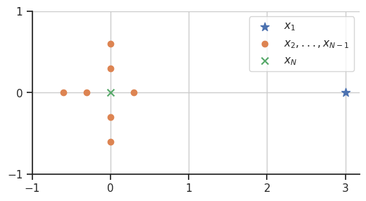
Refer to caption — Figure 1. Illustration of the proof of Proposition 3.4, for $d=2$ and $k=3$ , case $N=2\cdot d\cdot(k-1)+1$ $(=9)$ .

For the case $N<2\cdot d\cdot(k-1)+1$ , we assign less than $2\cdot d\cdot(k-1)-1$ points $x_{2},...,x_{N-1}$ between $\mathbf{0}$ and $\pm\mathbf{e_{s}}$ , such that $x_{N}$ is still part of all groups while $x_{1}$ is still furthest from all points.
For the case $N>2\cdot d\cdot(k-1)+1$ , we assign the additional points $x_{2\cdot d\cdot(k-1)+1},...,x_{N-1}$ to $-2\cdot\mathbf{e_{1}}$ which changes neither that $x_{N}$ is among the $k$ -nearest points of all $x_{2},...,x_{2\cdot d\cdot(k-1)}$ , nor that $x_{1}$ is furthest from all points. ∎

Proposition 3.5 (Strong consistency of $\mathcal{X}$ -based $k$ -NN).
Assume $\mathcal{X}=\mathbb{R}^{d}$ with a metric $d_{\mathcal{X}}$ s.t. $(\mathcal{X},d_{\mathcal{X}})$ is separable, a predictor $\hat{p}:\mathcal{X}\to[0,1]$ , and a joint distribution $P$ on random variables $(X,Y)$ with values in $\mathcal{X}\times\{0,1\}$ . Denote the Bayes-optimal predictor by $p(x):=\mathbb{E}[Y|X=x]$ . Then

\mathbb{E}_{P}\left[\left|c(I_{X}^{N}){-}(\hat{p}(X)-p(X))\right|\right]\to 0\text{ almost surely as }N\to\infty,

where $I_{x}^{N}$ denotes the set of $k$ -NN of $x$ with $k\to\infty$ , $\frac{k}{N}\to 0$ for $N\to\infty$ .

Proof.

We can reduce our problem to the consistency of $k$ -NN estimators; in the following we adapt notation used in (Devroye et al. 1994): For fixed $\hat{p}$ , define $Z:=\hat{p}(X)-Y$ . Then $Z$ is bounded and we get a joint distribution $(X,Z)$ , a true calibration error $m(x)=\mathbb{E}[Z|X=x]=\hat{p}(X)-p(x)$ and an estimator $m_{N}(x):=c(I_{x}^{k})=\frac{1}{k}\sum_{i\in I_{x}^{k}}z_{i}$ with $z_{i}=\hat{p}(x_{i})-y_{i}$ .
Then by Theorem 1 from (Devroye et al. 1994), we get $\mathbb{E}\left[\left|m_{N}(x)-m(x)\right|\right]\to 0$ with probability 1 as $N\to\infty$ , which is our desired result.¹⁸¹⁸ 18 Note that we are glossing over the details of tie-breaking, as the expectation is also an expectation over a supporting variable $Z$ . ∎

Proposition 3.6 (Strong consistency of $\mathcal{X}$ -based kernels).
Assume $\mathcal{X}=\mathbb{R}^{d}$ , a predictor $\hat{p}:\mathcal{X}\to[0,1]$ , and a joint distribution $P$ on random variables $(X,Y)$ with values in $\mathcal{X}\times\{0,1\}$ . Denote the Bayes-optimal predictor by $p(x):=\mathbb{E}[Y|X=x]$ . Then

\mathbb{E}_{P}\left[\left|C(q_{X}^{\gamma}){-}(\hat{p}(X)-p(X))\right|\right]\to 0\text{ almost surely as }N\to\infty,

Proof.

We can reduce this problem to the consistency of kernel estimators; in the following, we adapt the notation used in (Greblicki et al. 1984), analogously to the proof of Proposition 3.5: For fixed $\hat{p}$ , define $Z:=\hat{p}(X)-Y$ . Then $Z$ is bounded and we get a joint distribution of $(X,Z)$ , a true calibration error $m(x)=\mathbb{E}[Z|X=x]=\hat{p}(x)-p(x)$ and an estimator $m_{N}(x):=C(q_{x}^{\gamma})=\sum_{i=1}^{N}q_{x}^{\gamma}(x_{i})\cdot z_{i}$ with $z_{i}=\hat{p}(x_{i})-y_{i}$ .
Additional constraints on $k$ are that

c_{1}\cdot H(\|x\|_{s})\leq k(x)\leq c_{2}\cdot H(\|x\|)\quad\text{and}\quad c_{3}\cdot\mathbf{1}_{\|x\|\leq r}(x)\leq k(x)

for $c_{1},c_{2},c_{3},r$ positive constants, and $H$ a bounded decreasing Borel function in $[0,\infty)$ such that $t^{d}H(t)\to 0$ as $t\to\infty$ .
Then by Corollary 1 from (Greblicki et al. 1984), we get $\mathbb{E}\left[\left|m_{N}(x)-m(x)\right|\right]\to 0$ with probability 1 as $N\to\infty$ , which is our desired result. ∎

For Proposition 5.1 (restated below), we need some prerequisites.
The Quadrangle Theorem of (Rockafellar and Uryasev 2013) is stated in terms of two classes of agglomeration functions, for which we require the following further axiom for agglomeration functions $\mathsf{R}$ and $C\in\mathcal{L}^{2}(J)$ :
A7 Agreement $C=\alpha\in\mathbb{R}\text{ constant }\Rightarrow\mathsf{R}(C)=\alpha$ .

Definition 13 (Regular Risk Measures).

A regular risk measure (RRM) is an agglomeration function satisfying A7, Aversity and Convexity (cf. footnotes 12, 15).

Definition 14 (Regular Deviation Measures).

A regular deviation measure (RDM) is an agglomeration function satisfying A6 and Convexity.

Now Rockafellar and Uryasev 2013 establish that

(A)

A convex agglomeration function satisfies A2 if and only if it satisfies A7.
(B)

Regular deviation measures $\mathsf{D}$ stand in a one-to-one relationship with regular risk measures $\mathsf{R}$ via

(42) $\mathsf{R}(C)=\mathbb{E}[C]+\mathsf{D}(C).$
(C)

$\mathsf{R}$ satisfies A3 if and only $\mathsf{D}$ does.
(D)

$\mathsf{R}$ satisfies A1 if and only if $\mathsf{D}$ satisfies $\mathsf{D}(C)\leq\sup C-\mathbb{E}[C]\ \forall C\in\mathcal{L}^{2}(J)$ .

Furthermore, Artzner et al. 1999 establish that

(E)

An agglomeration satisfying A3 is convex if and only if it satisfies A4.

Lastly, it is easy to see that

(F)

For an RRM $\mathsf{R}$ and its corresponding RDM $\mathsf{D}$ , if one is law-invariant, then so is the other.

Proposition 5.1 (Relation between CRMs and FDMs).

a)

Agglomeration functions $\mathsf{D}$ satisfying A3-A6 stand in a one-to-one relationship with agglomeration functions $\mathsf{R}$ satisfying A2-A5 and Aversity (the property that $\mathsf{R}(C)>\mathbb{E}[C]$ if $C\in\mathcal{L}^{2}(J)$ is not constant) via

(43) $\mathsf{R}(C)=\mathbb{E}[C]+\mathsf{D}(C).$
b)

A law-invariant CRM induces an FDM via (43) iff it is averse.
c)

An FDM induces a law-invariant CRM via (43) iff it satisfies $\mathsf{D}(C)\leq\sup C-\mathbb{E}[C]\ \forall C\in\mathcal{L}^{2}(J)$ .

Proof.

a)

An agglomeration function $\mathsf{D}$ satisfying A3-A6 satisfies Convexity by (E) and is thus an RDM. An agglomeration function $\mathsf{R}$ satisfying A2-A5 and Aversity satisfies A7 by (A) and Convexity by (E) and is thus an RRM. The result follows from (B), (C), and (F).
b)

This result follows directly from a) via the definitions of CRMs and FDMs.
c)

This result follows from a) and (D).

∎

Appendix D Partitions with Non-uniform Measures

For groupings based on partitions, we may take group size into account in a different way compared to that in Sections 4 & 5.1 and Appendix A: Instead of counting groups multiple times in a grouping (as in (14) for the ECE), we may make use of the measure on the measure space $J$ , call it $\mu$ , that we have so far assumed to be uniform and thus left implicit (see the paragraph above Definition 1). This alternative formalisation, which encodes the information about group weights in the measure rather than in the multiplicities of the groups, has the advantage that we can treat partition-based groupings as partitions of the dataset since each datapoint is then a member of exactly one element of the grouping. Using this alternative encoding of group weights, we provide an additional result that strengthens the choice of axioms in Sections 4 and 5.1, in particular Convexity (cf. footnote 12) and thereby also Subadditivity: We show that the proposed global scores cannot decrease when making partitions finer, that is, when further subdividing the groups (Definition 15 below). This can be seen as an extension of Proposition 3.2 that also takes into account properties of the considered agglomeration functions.

Definition 15 (Refinement, Finer, Coarser).

For two partitions $\mathcal{P}_{1},\mathcal{P}_{2}$ of some set $\mathcal{I}$ , the former is finer than or a refinement of the latter if every element of $\mathcal{P}_{1}$ is a subset of some element of $\mathcal{P}_{2}$ . This is equivalent to saying that $\mathcal{P}_{2}$ is coarser than $\mathcal{P}_{1}$ .

Proposition 15 (Finer partitions have higher scores).

Take some $\hat{p}:\mathcal{X}\to[0,1]$ , an agglomeration function $\mathsf{R}$ , and a dataset $\{(x_{i},y_{i})\}_{i\in\mathcal{I}}$ with $\mathcal{I}:=\{1,...,N\}$ .

a)

If $\mathsf{R}$ is law-invariant and convex, plus if $\mu$ is given by the empirical distribution (that is, group errors are weighted by the size of the groups), then finer partitions cannot have lower global scores of raw (signed) errors than coarser ones.
b)

If $\mathsf{R}$ is monotonic, law-invariant, and convex, plus if $\mu$ is given by the empirical distribution, then finer partitions cannot have lower global scores of absolute errors than coarser ones.

Proof.

a)

Take two partitions $\mathcal{P}_{1},\mathcal{P}_{2}$ of $\mathcal{I}$ s.t. they contain the same sets except for some $I\in\mathcal{P}_{1}$ and $I_{k},I_{l}\in\mathcal{P}_{2}$ with $I=I_{k}\cup I_{l}$ . That means that $\mathcal{P}_{2}$ is (slightly) finer than $\mathcal{P}_{1}$ since $I\in\mathcal{P}_{1}$ is further subdivided. Now let $J_{1}$ and $J_{2}$ denote the index sets of the partitions $\mathcal{P}_{1}$ and $\mathcal{P}_{2}$ , equipped with the measure $\mu$ given by the empirical data distribution – this means $\forall i\in\{1,2\},j\in J_{i}:\mu(j)=\frac{|I_{j}|}{|\mathcal{I}|}$ . We slightly abuse notation by overloading $\mu$ and $\mathsf{R}$ to denote the measures and agglomeration functions, respectively, on both $J_{1}$ and $J_{2}$ .¹⁹¹⁹ 19 Since $\mu$ is defined through the empirical distribution, the measure on $J_{1}$ and the one on $J_{2}$ are in some sense ’the same’ despite operating on different spaces. Furthermore, to compare global scores on different partitions, we need some principle to identify agglomeration functions $\mathsf{R}$ operating on different measure spaces. In the literature on inequality indices, this is done explicitly or implicitly through a shared functional form of inequality measures that can be applied to different population sizes. Here, this can be done even more naturally since agglomeration functions satisfying Law Invariance only depend on the distribution of errors, not on the particularities of the measure spaces. Focusing on distributions as inputs, we can identify agglomeration functions on $J_{1}$ and on $J_{2}$ with each other and understand LI as a property of such functions operating on distributions.
Let $C_{1},C_{2}\in\mathcal{L}^{2}(J_{1}),\mathcal{L}^{2}(J_{2})$ denote the raw calibration errors of $\hat{p}$ under $\mathcal{P}_{1},\mathcal{P}_{2}$ , respectively. Then

(44) $\frac{\mu(I_{k})}{\mu(I)}c(I_{k})+\frac{\mu(I_{l})}{\mu(I)}c(I_{l})=c(I)$

by definition of $c(\cdot)$ and $\mu$ (given $I=I_{k}\cup I_{l}$ , similar to Proposition 3.2b).

Now let $\tilde{C}_{1}\in\mathcal{L}^{2}(J_{2})$ be equal to $C_{2}$ except that for $k,l\in J_{2}$ (corresponding to $I_{k},I_{l}$ ), $\tilde{C}_{1}(k)=\tilde{C}_{1}(l)=c(I)$ . That is, $\tilde{C}_{1}$ is defined on the same space as $C_{2}$ (namely $J_{2}$ ) while having the same distribution as $C_{1}$ , given that $\frac{|I|}{|\mathcal{I}|}=\frac{|I_{k}|+|I_{l}|}{|\mathcal{I}|}$ . Thus, by LI, $\mathsf{R}(C_{1})=\mathsf{R}(\tilde{C}_{1})$ (cf. footnote 19).

To prove $\mathsf{R}(C_{1})\leq\mathsf{R}(C_{2})$ , it remains to be shown that $\mathsf{R}(\tilde{C}_{1})\leq\mathsf{R}(C_{2})$ .

By (Bellini et al. 2021) Proposition 5.6, if $\mathsf{R}$ is LI and convex then it is dilatation monotone, that is,

(45) $\mathsf{R}(\mathbb{E}[C_{2}\ |\ \mathcal{G}])\leq\mathsf{R}(C_{2})$

for any sub- $\sigma$ -algebra $\mathcal{G}$ . This is precisely the property that we need, essentially meaning that by making a partition coarser, the agglomerated score may only decrease.

Since in our case, ${C}_{1}$ ad $C_{2}$ are identical except that the former combines $I_{k}$ and $I_{l}$ into $I$ by averaging their scores as stated in (44), we have $\tilde{C}_{1}=\mathbb{E}[C_{2}\ |\ \mathcal{G}]$ for $\mathcal{G}$ denoting the $\sigma$ -algebra induced by the (coarser) partition $\mathcal{P}_{1}$ . Therefore, by Dilatation Monotonicity, $\mathsf{R}(\tilde{C}_{1})\leq\mathsf{R}(C_{2})$ .

Since we can represent any refinement of a partition on a finite set through steps where one set is split into two (as done here for $I=I_{k}\cup I_{l}$ ), the result holds for any two partitions where one is finer than the other.
b)

Take the same $\mathcal{P}_{1},\mathcal{P}_{2},I,I_{k},I_{l},\mu$ as above.

Now let $C_{1},C_{2}\in\mathcal{L}^{2}(J_{1}),\mathcal{L}^{2}(J_{2})$ denote the absolute calibration errors of $\hat{p}$ under $\mathcal{P}_{1},\mathcal{P}_{2}$ , respectively.
As in Proposition 3.2b), introducing $|\cdot|$ to (44) yields

(46) $\frac{\mu(I_{k})}{\mu(I)}|c(I_{k})|+\frac{\mu(I_{l})}{\mu(I)}|c(I_{l})|\geq|c(I)|.$

Define $\tilde{C}_{1}$ as above except that, given that we now consider absolute errors, $\tilde{C}_{1}(k)=\tilde{C}_{1}(l)=|c(I)|$ . Then $\tilde{C}_{1}$ again has the same distribution as $C_{1}$ and thus, by LI, $\mathsf{R}(C_{1})=\mathsf{R}(\tilde{C}_{1})$ .

For the case of equality in (46), we can show $\mathsf{R}(\tilde{C}_{1})\leq\mathsf{R}(C_{2})$ as in part a).

For the case of strict inequality, define $C_{3}\in\mathcal{L}^{2}(J_{2})$ to be equal to $C_{2}$ except that $C_{3}(k)<C_{2}(k)$ s.t. $\mathbb{E}_{\mu}[C_{3}]=\mathbb{E}_{\mu}[\tilde{C}_{1}]$ . Then $\mathsf{R}(\tilde{C}_{1})\leq\mathsf{R}(C_{3})$ by Dilatation Monotonicity as in part a) and $\mathsf{R}(C_{3})\leq\mathsf{R}(C_{2})$ by Monotonicity.

Thus, we again get $\mathsf{R}(C_{1})\leq\mathsf{R}(C_{2})$ in either case which proves the result.

∎

(33)	$\displaystyle\|c(I_{1}\cup I_{2})\|$	$\displaystyle=\ \frac{1}{\|I_{1}\cup I_{2}\|}\left\lvert\sum_{i\in I_{1}\cup I_{2}}\hat{p}(x_{i})-y_{i}\right\rvert$
(34)		$\displaystyle=\ \frac{1}{\|I_{1}\|+\|I_{2}\|}\left\lvert\sum_{i\in I_{1}}[\hat{p}(x_{i})-y_{i}]+\sum_{i\in I_{2}}[\hat{p}(x_{i})-y_{i}]\right\rvert$
(35)		$\displaystyle\leq\ \frac{1}{\|I_{1}\|+\|I_{2}\|}\left(\left\lvert\sum_{i\in I_{1}}[\hat{p}(x_{i})-y_{i}]\right\rvert+\left\lvert\sum_{i\in I_{2}}[\hat{p}(x_{i})-y_{i}]\right\rvert\right)$
(36)		$\displaystyle\leq\ \frac{\alpha\cdot\|I_{1}\|+\beta\cdot\|I_{2}\|}{\|I_{1}\|+\|I_{2}\|}.$

Abstract.

Keywords:

1. Introduction

2. Calibration From the Ground Up

2.1. From individuals to groups

2.2. Conventional understanding of calibration

3. Grouping Choices

3.1. Vicinity-based grouping principles

Proposition 0 (Cohesion in domain and codomain).

3.2. Group size

Proposition 0 (Advantage of smaller groups: Resolution).

Proposition 0 (Advantage of larger groups: Variance).

3.3. Alternative grouping structures

Proposition 0 (Group overlap for 𝒳\mathcal{X}-based kk-NN).

Proposition 0 (Strong consistency of 𝒳\mathcal{X}-based kk-NN).

Proposition 0 (Strong consistency of 𝒳\mathcal{X}-based kernels).

4. Global Calibration Scores

Definition 1 (Agglomeration Function).

Definition 2 (Coherent Risk Measure; (Artzner et al. 1999)).

Definition 3 (Conditional Value at Risk; (Artzner et al. 1999)).

5. Calibration-based Notions of Fairness

5.1. Global fairness scores

Definition 4 (Fairness Deviation Measures).

Proposition 4 (Relation between CRMs and FDMs).

Example 5 (Fairness Deviation Measures).

5.2. Group fairness and individual fairness

6. Conclusion and Future Work

Acknowledgements.

References

Appendix A Established Calibration Scores

Appendix B On Group Cohesion and Topology

Definition 6 (Topology, Open set, Neighbourhood).

Example 7 (Trivial topology).

Example 8 (Induced topology, Standard topology on ℝd\mathbb{R}^{d}).

Definition 9 (Hausdorff space).

Definition 10 (Topological continuity).

Definition 11 (Connectedness).

Definition 12 (Path-connectedness).

Appendix C Proofs

Proof.

Proof.

Proof.

Proof.

Proof.

Proof.

Definition 13 (Regular Risk Measures).

Definition 14 (Regular Deviation Measures).

Proof.

Appendix D Partitions with Non-uniform Measures

Definition 15 (Refinement, Finer, Coarser).

Proposition 15 (Finer partitions have higher scores).

Proof.

Proposition 0 (Group overlap for $\mathcal{X}$ -based $k$ -NN).

Proposition 0 (Strong consistency of $\mathcal{X}$ -based $k$ -NN).

Proposition 0 (Strong consistency of $\mathcal{X}$ -based kernels).

Example 8 (Induced topology, Standard topology on $\mathbb{R}^{d}$ ).