Standing Between Past and Future: Spatio-Temporal Modeling for
Multi-Camera 3D Multi-Object Tracking
Abstract
This work proposes an end-to-end multi-camera 3D multi-object tracking (MOT) framework. It emphasizes spatio-temporal continuity and integrates both past and future reasoning for tracked objects. Thus, we name it “Past-and-Future reasoning for Tracking” (PF-Track). Specifically, our method adopts the “tracking by attention” framework and represents tracked instances coherently over time with object queries. To explicitly use historical cues, our “Past Reasoning” module learns to refine the tracks and enhance the object features by cross-attending to queries from previous frames and other objects. The “Future Reasoning” module digests historical information and predicts robust future trajectories. In the case of long-term occlusions, our method maintains the object positions and enables re-association by integrating motion predictions. On the nuScenes dataset, our method improves AMOTA by a large margin and remarkably reduces ID-Switches by 90% compared to prior approaches, which is an order of magnitude less. The code and models are made available at https://github.com/TRI-ML/PF-Track.
1 Introduction
Reasoning about object trajectories in 3D is the cornerstone of autonomous navigation. While many LiDAR-based approaches exist simpletrack; zaech2022learnable; weng2020gnn3dmot, their applicability is limited by the cost and reliability of the sensor. Detecting, tracking, and forecasting object trajectories only with cameras is hence a critical problem. Significant progress has been achieved on these tasks separately, but they have been historically primarily studied in isolation and combined into a full-stack pipeline in an ad-hoc fashion.
In particular, 3D detection has attracted a lot of attention bevformer; detr3d; petr; huang2021bevdet; li2022bevdepth, but associating these detections over time has been mostly done independently from localization scheidegger2018mono; luiten2020track; hu2022monocular. Recently, a few approaches to end-to-end detection and tracking have been proposed, but they operate on neighboring frames and fail to integrate longer-term spatio-temporal cues mutr3d; cc3dt; marinello2022triplettrack; chaabane2021deft. In the prediction literature, on the other hand, it is common to assume the availability of ground truth object trajectories and HD-Maps chang2019argoverse; nuscenes; wilson2021argoverse; ettinger2021large. A few attempts for a more realistic evaluation have been made ivanovic2021heterogeneous; gu2022vip3d, focusing only on the prediction performance.

In this paper, we argue that multi-object tracking can be dramatically improved by jointly optimizing the detection-tracking-prediction pipeline, especially in a camera-based system. We provide an intuitive example from our real-world experiment in Fig. 1. At first, the pedestrian is fully visible, but a model with only single-frame information makes a prediction with large deviation (frame in Fig. 1). After this, integrating the temporal information from the past gradually corrects the error over time (frame in Fig. 1), by capitalizing on the notion of spatio-temporal continuity. Moreover, as the pedestrian becomes fully occluded (frame in Fig. 1), we can still predict their location by using the aggregated past information to estimate a future trajectory. Finally, we can successfully track the pedestrian on re-appearance even on a different camera via long-term prediction, resulting in correct re-association (frame in Fig. 1). The above robust spatio-temporal reasoning is enabled by seamless, bi-directional integration of past and future information, which starkly contrasts with the mainstream pipelines for vision-based, multi-camera, 3D multi-object tracking (3D MOT).
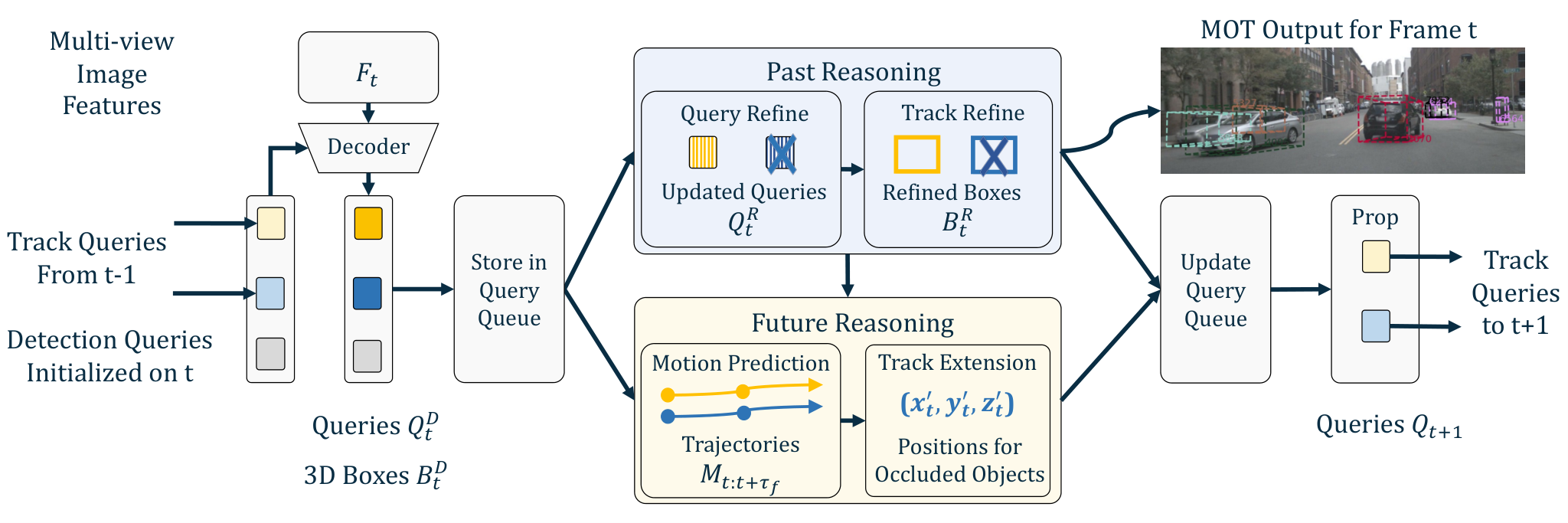
To this end, we propose an end-to-end framework for joint 3D object detection, tracking, and trajectory prediction for the task of 3D MOT, as shown in Fig. 2, adopting the “tracking by attention” trackformer; motr; mutr3d paradigm. Compared to our closest baseline under the same paradigm mutr3d, we are different in explicit past and future reasoning: a 3D object query consistently represents the object over time, propagates the spatio-temporal information of the object across frames, and generates the corresponding bounding boxes and future trajectories. To exploit spatio-temporal cues, our algorithm leverages simple attention operations to capture object dynamics and interactions, which are then used for track refinement and robust, long-term trajectory prediction. Finally, we close the loop by integrating predicted trajectories back into the tracking module to replace missing detections (e.g., due to an occlusion). To highlight the capability of joint past and future reasoning, our method is named “Past-and-Future reasoning for Tracking” (PF-Track).
We provide a comprehensive evaluation of PF-Track on nuScenes nuscenes and demonstrate that joint modeling of past and future information provides clear benefits for object tracking. In particular, PF-Track decreases ID-Switches by over 90% compared to previous multi-camera 3D MOT methods.
To summarize, our contributions are as follows.
- 1.
We propose an end-to-end vision-only 3D MOT framework that utilizes object-level spatio-temporal reasoning for both past and future information.
- 2.
Our framework improves the quality of tracks by cross-attending to features from the “past.”
- 3.
We propose a joint tracking and prediction pipeline, whose constituent part is “Future Reasoning”, and demonstrate that tracking can explicitly benefit from long-term prediction into the “future.”
- 4.
Our method establishes new state-of-the-art on large-scale nuScenes dataset nuscenes with significant improvement for both AMOTA and ID-Switch.
2 Related Work
LiDAR-based 3D MOT. The majority of prior works in 3D MOT leverage the LiDAR modality. Due to the recent advances in LiDAR-based 3D detection yin2021center; pointpillars, especially the reliable range information, most state-of-the-art 3D MOT algorithms adopt a “tracking-by-detection” paradigm ab3dmot. Given single frame detection outputs, different approaches have been proposed to improve data association simpletrack; zaech2022learnable; weng2020gnn3dmot, motion propagation chiu2021probabilistic; centertrack, and life cycling simpletrack; wang2021immortal. However, most of these works assume the localization accuracy of detection output. Therefore, data association is usually conducted based on location, optionally combined with abstracted object attributes (e.g., 3D intersection over untion (3D IoU) ab3dmot, 3D generalized intersection over union (GIoU) simpletrack, and L2 distance yin2021center). This bias causes the proposed systems to be fragile when migrated into the camera modality, where 3D detection suffers from higher localization uncertainty. Although the latest methods incorporate learning-based algorithms to improve association with high-fidelity features such as low-level features from point clouds stearns2022spot or intermediate features from cameras chiu2021probabilistic, these approaches are built on top of the LiDAR-based frameworks and share their dependence on localization quality.
Camera-based 2D MOT. Camera-based multi-object tracking in 2D is a classic task in computer vision. Dominated by “tracking by detection” paradigm bewley2016simple, 2D MOT has seen more success in leveraging high-fidelity features wojke2017simple; tang2017multiple; zhang2021fairmot; peng2021transmot. Earlier works like DeepSORT wojke2017simple leveraged intermediate features from a deep net to measure appearance similarity. FairMOT zhang2021fairmot employed an additional Re-ID branch to learn discriminative features in a detection network. TransMOT peng2021transmot proposed to incorporate spatio-temporal features using a graph network.
Camera-based 3D MOT. Camera-based 3D MOT has recently drawn more attention in autonomous driving applications thanks to advances in monocular depth estimation dorncvpr; packnet; godard2019digging and image-based 3D object detection CaDDN; park2021dd3d; bevformer; petrv2; li2022bevdepth; huang2021bevdet; petr; detr3d; wang2021fcos3d. Early methods adapt the 2D MOT algorithms and lift the 2D tracking result using monocular depth centertrack; tokmakov2021learning. More recent approaches employ additional 3D information in data association scheidegger2018mono; luiten2020track; hu2022monocular. luiten2020track proposes to leverage 3D reconstruction, and hu2022monocular augments the 2D Re-ID features with 3D attributes (e.g. depth and orientation). CC-3DT cc3dt merges the multi-view camera features for identical objects to improve the cross-time cross-view association. However, considering or correcting the high uncertainty and bias in camera-based 3D detection has been less explored. In this work, we leverage long-term object reasoning, especially past reasoning, to improve the quality of 3D bounding boxes.
Tracking by Attention. A rising trend in MOT is the “tracking by attention” paradigm motr; sun2020transtrack; trackformer; mutr3d, inspired by the novel transformer-based detection architecture DETR carion2020end. MOTR motr and Trackformer trackformer extended the query-based detection framework in DETR carion2020end by propagating queries across different frames. In this paradigm, the data association is replaced by “detection” in the current frame with a set of track queries. MUTR3D mutr3d proposes the first framework applying this paradigm to the 3D MOT domain. It uses a 3D track query to jointly model object features across timestamps and multi-views. Despite its improvement at the time, MUTR3D mostly follows the designs of 2D MOT methods and does not include special treatment to improve the localization quality of tracks and better propagate the queries to future frames. Our proposed algorithm also operates in the “tracking by attention” paradigm but extends the temporal horizon of existing methods. In particular, we demonstrate that joint past and future reasoning can improve the tracking framework by providing a strong spatio-temporal object representation.
Motion Prediction. Predicting agent trajectories is critical for self-driving ngiam2021scene; gao2020vectornet; yuan2021agentformer; ivanovic2019trajectron; salzmann2020trajectron++; liu2021multimodal; shi2022motion. The most common setting is to predict from clean tracks annotated by humans or auto-labeling sun2020scalability; ettinger2021large; chang2019argoverse; wilson2021argoverse. Numerous studies focus on end-to-end prediction from perception weng2022mtp; weng2022whose; weng2021inverting; fiery; beverse; casas2021mp3; luo2018fast; phillips2021deep; shah2020liranet; liang2020pnpnet; peri2022forecasting; akan2022stretchbev, especially how to improve motion prediction directly from perception. However, our objective is different: Could a motion prediction model benefit 3D MOT? In the 2D setting, this problem has received only limited attention recently dendorfer2022quo. Our algorithm advances this research into a more challenging multi-camera, 3D scenario and does not require explicit re-identification.
3 Method: PF-Track
This section introduces our novel 3D multi-object tracking framework, shown in Fig. 2. It is centered around explicit past and future modeling of object trajectories in an end-to-end framework. We first provide an overview of the pipeline in Sec. 3.1, and then explain how to efficiently leverage “Past” (Sec. 3.2) and “Future” (Sec. 3.3) information. Finally, we summarize the losses used in our framework in Sec. 3.4.
3.1 PF-Track Pipeline
Our proposed PF-Track iteratively uses a set of object queries mutr3d; motr; trackformer to tackle multi-view, multi-object, 3D tracking. At each timestamp , given images from surrounding cameras, the objective of 3D MOT is to generate object detections with consistent IDs across frames, denoted by , where is an object ID.
3D Object Queries. The entry point in our framework is to receive the object queries propagated from the previous frame (yellow and blue squares in Fig. 2), which represent the tracked objects:
| (1) |
Such a query-based design naturally addresses the task of tracking as the queries carry the identity of objects over time. Apart from queries from the previous frame that represent tracked instances, we also add a fixed number of detection queries (gray squares in Fig. 2) to discover new objects. In practice, we use 500 detection queries initialized as learnable embeddings.
Each query represents a unique 3D object with a feature vector and a 3D location : . Here we highlight that the query position is an active participant in decoding the bounding boxes of objects below.
Decoder. To predict 3D bounding boxes and update queries with the latest image inputs, PF-Track adopts an attention-based detection architecture carion2020end; zhu2020deformable to decode image features with object queries:
| (2) |
where and are the detected 3D bounding boxes and updated query features, respectively. In the decoding process, the decoder lifts the 3D positions of queries into positional embeddings to concentrate on the image regions relevant to the spatial locations of the objects. While the design of PF-Track is agnostic to query-based detection algorithms, we mainly adopt a current state-of-the-art 3D detector, PETR petr, for experiments.
Past and Future Reasoning for Refinement and Propagation. After decoding the queries and boxes from single-frame image features, PF-Track conducts past and future reasoning sequentially to (1) refine the current detections into and queries into . ( is short for “refinement.”); (2) propagate the queries to the next timestamp with the predicted motions.
“Past Reasoning” is the component that aggregates the information from previous frames to generate refined queries and refined bounding boxes :
| (3) |
In practice, the historical queries come from a query queue that maintains the queries from past frames ( for “history”).
After past reasoning, the “Future Reasoning” module improves the coherence of object positions from the aspect of query propagation. It achieves this by forecasting the motions up to frames ( for “future”) and transforms the positions of queries accordingly:
| (4) |
Specifically, future reasoning extracts the object dynamics from historical query features to predict the trajectories . The single-step movement is leveraged to propagate the current queries to the next timestamp, and long-term trajectories are used for addressing occlusions. The “Track Extension” in Fig. 2 refers to occlusion reasoning through the predicted trajectories.
PF-Track iteratively executes the above procedures. The refined 3D bounding boxes are the output for 3D MOT.
3.2 Past Reasoning
To address the uncertainty of detection in vision-only 3D localization, past reasoning focuses on two aspects: (1) enhancing the query features by attending to historical embeddings; (2) refining the tracks by adjusting the bounding boxes using the improved query features.
Query Refinement: from to . We first apply attention across the time and instance axes to explicitly update the query features with historical information, as illustrated in Fig. 3. “Cross-frame” attention encourages the interplay of features within a history window of frames per object:
| (5) |
where, converts the timestamps into positional embedding, and the history frames with empty features are ignored for attention computation.
Then past reasoning applies “cross-object” attention to incorporate the context information and encourage more discriminative feature representation for each object. In particular, cross-object attention (Fig. 3, right) further updates the query features via
| (6) |
where cross-object attention exchanges the features of objects guided by their 3D positional embedding . The final output becomes the refined feature vectors in queries .
As a brief remark, decoupling cross-frame and cross-object attention exhibits two advantages. Firstly, separating attention across frames (cross-frame) and objects (cross-object) enables us to design specialized positional encoding of time and locations for each of them. Secondly, it decreases the computational complexity from for the global cross-attention to , which is significantly less. Our design is also closely related to how motion prediction methods ngiam2021scene; gao2020vectornet model spatial-temporal relationships.
Track Refinement: from to . With the queries refined by historical information, past reasoning further uses track refinement to improve the 3D bounding box quality. As specified in Eqn. 7, we apply a multi-layer perceptron (MLP) to predict the updated properties of objects, including center residuals (), size (), orientations (), velocities (v), and scores ():
| (7) |
These are then used to adjust the original boxes as follows:
| (8) |
resulting in , which is the final model output at frame .
3.3 Future Reasoning
“Future Reasoning” concentrates on improving the propagation of queries across frames to benefit spatio-temporal coherence. It first learns a trajectory prediction, which is used for moving queries across adjacent frames. Then future reasoning exploits the predicted long-term trajectories for maintaining the positions of occluded or noisy tracks.
Motion Prediction. Trajectory prediction supervises the model’s ability to capture object movements and is further beneficial for propagating query positions across timestamps. Similar to past reasoning, our future reasoning model adopts a simple attention-based architecture. Firstly, we generate the motion embeddings for timestamps with a cross-frame attention:
| (9) |
where are initialized as zeros, and historical features serve as the source of information. Then the movement at every timestamp is decoded by an MLP:
| (10) |
and the object trajectory in the 3D space can be recovered by combining these frame-level outputs. Our architecture is inspired by SceneTransformer ngiam2021scene, which also employs a fully-attention-based architecture.
The predicted trajectories have better fidelity compared to the velocities v predicted by the decoder in and . Thus, we can propagate the positions of queries by adding a single step of the trajectory:
| (11) |
Track Extension. To handle occlusions or noisy observations, we propose to extend the tracks using the predicted trajectories. In particular, we replace missing or low-confidence detections with the output of our motion prediction module, which is initialized from confident observations. Previous 3D MOT approaches either terminate the tracks or prolong them with heuristic motion models (e.g. Kalman filters) under such conditions. However, these solutions both could lead to ID-Switches due to “early termination” simpletrack or false associations. In contrast, our learnable motion prediction module and track extension strategy are more accurate and robust.
We visualize the high-level intuition in Fig. 4 and provide more details in Sec. B.2 (appendix). In Fig. 4, the long-term trajectories assist the propagation of the yellow instance (bottom row). When PF-Track encounters noisy observation or occlusion cases, it relies on the motion predictions from previous confident frames to simulate the movements of occluded objects. In extreme cases, our model is able to handle occlusion length of frames. Our ablation study in Sec. 4.4 demonstrates that track extension can decrease ID-Switch by a large margin. To the best of our knowledge, we are the first to incorporate long-term prediction into a query-based framework and address occlusion without explicit re-identification.

3.4 Loss Functions
Our final loss function is defined as follows:
| (12) | ||||
where and are focal loss lin2017focal with the coefficients of and . They supervise the classification scores of and , respectively. and are both L1 loss applied to and for bounding box regression. Their coefficients are and . The motion prediction loss is an L1 loss between the movements of predicted and ground truth trajectories, weighted by . The ground truth assignment couples a query with a consistent ground truth instance over time to encourage ID consistency. We discuss more details in Sec. B (appendix).
4 Experiments
4.1 Datasets and Metrics
Datasets. We conduct experiments on the large-scale self-driving dataset nuScenes nuscenes. It contains 1,000 video sequences with multiple modalities, including RGB images from 6 surrounding cameras, and point clouds from LiDAR and Radar. In this paper, we use camera sensors only. Every sequence spans roughly 20 seconds with keyframes annotated at 2Hz. The dataset provides 1.4M 3D bounding boxes covering 10 types of common objects on the road. For the tracking task, nuScenes selects a subset of 7 mobile categories, such as cars, pedestrians, and motorcycles, and excludes static objects like traffic cones.
Metrics. We strictly follow the official evaluation metrics for multi-object tracking tasks from nuScenes. It modifies CLEAR MOT metrics bernardin2008evaluating by considering multiple recall thresholds. The main metric is “Average Multi-Object Tracking Accuracy” (AMOTA) ab3dmot. Meanwhile, we also consider other analytical metrics such as “Identity Switches” (IDS) and “Average Multi-Object Tracking Precision” (AMOTP).
| AMOTA | AMOTP | RECALL | MOTA | IDS | |
| Validation Split | |||||
| DEFT chaabane2021deft | 0.201 | N/A | N/A | 0.171 | N/A |
| QD3DT hu2022monocular | 0.242 | 1.518 | 39.9% | 0.218 | 5646 |
| MUTR3D mutr3d | 0.294 | 1.498 | 42.7% | 0.267 | 3822 |
| TripletTrack marinello2022triplettrack | 0.285 | 1.485 | N/A | N/A | N/A |
| CC-3DT∗ cc3dt | 0.429 | 1.257 | 53.4% | 0.385 | 2219 |
| PF-Track-S (Ours) | 0.408 | 1.343 | 50.7% | 0.376 | 166 |
| PF-Track-F (Ours) | 0.479 | 1.227 | 59.0% | 0.435 | 181 |
| Test Split | |||||
| CenterTrack centertrack | 0.046 | 1.543 | 23.3% | 0.043 | 3807 |
| PermaTrack tokmakov2021learning | 0.066 | 1.491 | 18.9% | 0.060 | 3598 |
| DEFT chaabane2021deft | 0.177 | 1.564 | 33.8% | 0.156 | 6901 |
| QD3DT hu2022monocular | 0.217 | 1.550 | 37.5% | 0.198 | 6856 |
| MUTR3D mutr3d | 0.270 | 1.494 | 41.1% | 0.245 | 6018 |
| TripletTrack marinello2022triplettrack | 0.268 | 1.504 | 40.0% | 0.245 | 1144 |
| CC-3DT∗ cc3dt | 0.410 | 1.274 | 53.8% | 0.357 | 3334 |
| PF-Track-F (Ours) | 0.434 | 1.252 | 53.8% | 0.378 | 249 |
4.2 Implementation Details
Due to space limits, we clarify two training settings here and describe more implementation detail in Sec. B (appendix). In our implementation, every training sample contains three adjacent frames from different timestamps. However, it requires extensive computation as every frame contains six high-resolution images. Therefore, we adopt two settings that downsample images to different resolutions, motivated by PETR petr.
Full-resolution. On every time frame, we crop the raw resolution images, to , leaving the sky area out. However, training a multi-frame tracker on this resolution would not fit in a single A100 GPU. Thus, we first pretrain the backbone with single-frame detection for 24 epochs, following some previous works tokmakov2021learning. Then we fix the backbone and train the tracker on three-frame samples for another 24 epochs. We only use this setting for full model results indicated with “-F” in Tab. 1.
Small-resolution. We apply a small-resolution setting for all of our ablation analyses unless specified. In this setting, we downsample the cropped images to a resolution of . We first train a single-frame detection model for 12 epochs and then train the tracker on three-frame samples for another 12 epochs.
4.3 State-of-the-art Comparison on nuScenes
In Tab. 1, we compare our model performance with the other published camera-based 3D MOT algorithms on nuScenes. Our approach establishes a new state-of-the-art with significant improvements on every metric. Our AMOTA improves more than on the test set and on the validation set over the previous methods, including a very strong concurrent work cc3dt. It is worth noting that with more established tracks (higher recall), our ID-Switch number is only of previous methods eliminating more than of the ID-switching errors. This result indicates the strong association ability of our algorithm attributed to leveraging both past and future reasoning. The advantage of our model holds even when trained in the low-resolution setting, whereas most of the previous works use full-resolution.
4.4 Ablation Studies
| Index | Past | Future | AMOTA | AMOTP | IDS | ||
|---|---|---|---|---|---|---|---|
| QR | TR | Pred | Ext | ||||
| 1 | 0.368 | 1.421 | 507 | ||||
| 2 | ✓ | 0.378 | 1.414 | 453 | |||
| 3 | ✓ | ✓ | 0.380 | 1.408 | 400 | ||
| 4 | ✓ | 0.374 | 1.402 | 469 | |||
| 5 | ✓ | ✓ | 0.391 | 1.360 | 155 | ||
| 6 | ✓ | ✓ | ✓ | ✓ | 0.408 | 1.343 | 166 |
Efficacy of Past and Future Reasoning. In Tab. 2, we analyze the importance of individual modules for our model’s performance using the validation set of nuScenes. In particular, we evaluate the following variants. (1) Baseline. Our baseline is a “tracking by attention” model without explicit spatio-temporal reasoning (row 1). It is a strong baseline and outperforms prior work in Tab. 1. (2) Past Reasoning. We first analyze the effect of query refinement (row 2), which explicitly incorporates the historical queries via cross-attention. As illustrated, it improves the overall tracking quality. We then exploit the enhanced feature to refine the 3D bounding boxes of tracks (row 3). It decreases ID-Switch and AMOTP, which indicates that track refinement is useful for 3D MOT. (3) Future Reasoning. Next, we demonstrate that learning to predict object motion and propagate positions (row 4) is beneficial for modeling object dynamics and leads to improved tracking performance. In addition, using the long-term trajectory predictions to replace low-confidence localizations (row 5) results in a 67% drop in ID-Switches. (4) Joint Past and Future Reasoning. Finally, combining past and future reasoning into an end-to-end framework shown in Fig. 2 (row 6) allows our model to achieve top performance. This result confirms that past and future reasoning are mutually beneficial for 3D MOT.
Length of Track Extension. In Fig. 5, we analyze the effect of track extension length on AMOTA and ID-Switches using our best-performing full-resolution model on the validation split of nuScenes. Compared to not using the extension strategy (0.0s), prolonging the tracks strongly improves the performance up to 2 seconds. Then the metrics saturate because only a few objects reappear after such a long period. Please note that these improvements are achieved without explicit re-identification.


Length of Prediction in Future Reasoning. Next, we analyze how the prediction length changes the 3D MOT performance on nuScenes validation split in Tab. 3. Concretely, we train three different full-fledged models with the prediction length of 2.0, 3.0, and 4.0 seconds. AMOTA and ID-Switch indicate that 4.0s (8 frames) has a slight advantage over 2.0s (4 frames) and 3.0s (6 frames). This result indicates that learning trajectory forecasting with longer horizon benefits our 3D MOT framework.
| Length | Extention | AMOTA | AMOTP | IDS |
|---|---|---|---|---|
| 2.0s | ✗ | 0.392 | 1.376 | 604 |
| 2.0s | ✓ | 0.402 | 1.342 | 217 |
| 3.0s | ✗ | 0.392 | 1.372 | 540 |
| 3.0s | ✓ | 0.402 | 1.340 | 208 |
| 4.0s | ✗ | 0.391 | 1.387 | 471 |
| 4.0s | ✓ | 0.408 | 1.343 | 166 |
Comparison with “Tracking by Detection” Baselines. In Tab. 4, we compare the performance between our end-to-end framework and previous “tracking by detection” algorithms ab3dmot; simpletrack; yin2021center, which are strong baselines for LiDAR-based 3D MOT. For these experiments, we also use the validation split of nuScenes. For a fair comparison, we evaluate these methods with PETR petr detections and tune their hyper-parameters for AMOTA (shown in the table with “,” details are provided in Sec. B.4 (appendix). The results clearly demonstrate the advantages of our end-to-end approach compared to more traditional, modular frameworks, with improvements being especially significant on the ID-Switch metric.
| AMOTA | AMOTP | IDS | |
| AB3DMOT ab3dmot | 0.292 | 1.333 | 2419 |
| AB3DMOT ab3dmotΨ | 0.329 | 1.388 | 2677 |
| CenterPoint yin2021center | 0.233 | 1.270 | 2715 |
| CenterPoint yin2021centerΨ | 0.383 | 1.329 | 3082 |
| SimpleTrack simpletrack | 0.320 | 1.295 | 1606 |
| SimpleTrack simpletrackΨ | 0.402 | 1.324 | 2053 |
| PF-Track (Ours) | 0.408 | 1.343 | 166 |
| Method | ADE (@4.0s) | FDE (@4.0s) |
|---|---|---|
| LSTM chang2019argoverse | 2.32 | 2.87 |
| VectorNet gao2020vectornet | 2.01 | 2.48 |
| Velocity | 2.10 | 2.64 |
| PF-Track (Ours) | 1.88 | 2.38 |
Analysis on Prediction from Query Features. While our paper focuses on multi-object tracking, we additionally provide an analysis of prediction performance. We show that predicting end-to-end from object features is advantageous over predicting from low-level object states, such as center positions. Specifically, we train two motion prediction baselines, VectorNet gao2020vectornet and LSTM chang2019argoverse, using the true-positive tracks from PF-Track following previous studies luo2018fast, and report their results in the top rows of Tab. 5. As our method does not use HD-Maps, for a fair comparison, we exclude the parts of motion prediction algorithms that handle HD-Maps in these experiments. In addition, we report another baseline which uses the velocities predicted by our model’s decoder for trajectory prediction, assuming a constant velocity motion model (third row in Tab. 5). The evaluation metrics are “average displacement error” (ADE) and “final displacement error” (FDE), which are better with lower values. More details are in Sec. B.5 (appendix).
Tab. 5 compares the performance between the end-to-end PF-Track and the baselines described above on the validation split of nuScenes. With lower ADE and FDE, PF-Track has better trajectory quality. Our conclusions agree with previous studies gu2022vip3d; weng2022mtp; luo2018fast. More specifically, LSTM is a shallow model and unable to capture meaningful dynamics from noisy tracks; the stronger VectorNet model can perform better than the other baselines, but it is still worse than forecasting trajectories in an end-to-end framework, as proposed in our method.
4.5 Qualitative Results
We visualize the 3D MOT results in Fig. 6 by projecting 3D bounding boxes onto images. The colors of bounding boxes are randomly selected from a pool of seven colors according to their IDs, so that each object has a consistent color over time.
In the top row, we provide an overall visualization of multi-camera 3D MOT, focusing on front-left and front cameras. As clearly shown, PF-Track tracks objects coherently, especially for the pedestrians and vehicles shown on two separate cameras. In the bottom two rows of Fig. 6, we illustrate two examples of addressing occlusions. For both large (bus) and small (pedestrian) objects, our method propagates their positions during the occluded frames and successfully re-associates them on de-occlusion frames even on a different camera. We highlight that this is achieved without an explicit re-identification module.
5 Conclusions
This paper proposes a query-based end-to-end method for multi-camera 3D MOT that enhances spatio-temporal coherence. By past reasoning, our framework enhances the query features and track quality with historical information. By future reasoning, the predicted trajectories better propagate the queries across adjacent frames and occluded long-term periods. We also demonstrate that joint past and future reasoning further strengthens the tracker’s ability. Extensive evaluation of the large-scale nuScenes dataset demonstrates that our method is effective in providing coherent tracks.
Acknowledgement. This work was supported in part by Toyota Research Institute, NSF Grant 2106825, NIFA Award 2020-67021-32799, and the NCSA Fellows program.
Appendix
Our appendix describes the additional experimental analysis and implementation details. The catalog is as below:
- (A)
Video demo. We provide a demo for multi-camera 3D multi-object tracking (MOT) as explained in Sec. A.
- (B)
Implementation details. We explain the detailed model architecture, procedures for training and inference, and settings for ablation studies in Sec. B.
- (C)
Additional ablations. We provide more analysis and experimental results in Sec. C.
- (D)
Performance Verification. For checking the results, we provide the screenshot of the test split results for verification in Sec. E.
A Multi-camera Tracking Video Demo
Our demo video is at https://youtu.be/eJghONb2AGg. It contains:
- •
Visualization of 3D MOT results on both surrounding images and Bird’s-eye-view.
- •
Illustration for addressing occlusions.
- •
Qualitative results for predicted trajectories.
B Implementation Details
B.1 Model Architecture
We explain the design choices of PF-Track in the sections below. To provide a high-level view of the model, we enclose the config file in mmdetection3d mmdet3d2020 format in this supplementary material.
Backbone. We use VoVNetV2 lee2019energy as backbone. For the feature pyramid lin2017feature, the C5 feature (output of the 5-th stage) is upsampled and fused with C4 feature (output of the 4-th stage). To save GPU memory during training, we adopt the checkpointing trick chen2016training by default.
Detection head. We follow the design of PETR petr by setting the region to on the XY-axis and on the Z-axis. The centers of bounding boxes are normalized to , respectively. The detection head composes of 6 transformer decoder layers vaswani2017attention and 2 MLP heads for bounding box regression and classification. Each transformer decoder layer has an embedding dimension of 256 and a feedforward dimension of 2048. The dropout probability is 0.1. The MLP heads are both two-layer MLPs. The bounding box regression head predicts the centers , sizes , orientation, and velocities of objects, and the classification head returns the logits for every category.
PF-Track configurations. Our PF-Track uses a fixed number of 500 detection queries per frame. As for track queries, the training and inference procedures are different. Training protocol adds queries into the set of track queries once they become a positive match to the ground truth (2.0m), and a tracking query is kept associated with the ground truth of the same object. The inference protocol initializes the track queries if the corresponding confidence score is larger than 0.4. During the inference time, our model output at most 300 objects (same as detr3d; petr; mutr3d) and set a minimum score threshold of 0.2.
Past reasoning. The length of the query queue is 1.5 seconds ( frames) because each of our training samples has 3 frames. However, we emphasize that PF-Track is able to aggregate historical information from the entire video during the inference time because the past reasoning module is recurrent. Concretely, the queries at frame attend to frames , and the queries at frame , in turn, attend to frames , and so on. Thus, the queries at frame have access to information from all the previous frames.
For cross-frame and cross-frame attention, we employ two transformer decoder layers for them each. Every transformer decoder layer has an embedding dimension of 256, and a feedforward dimension of 2048. Same as the transformer layers in the detection head, these two layers also have a dropout probability of 0.1. The track refinement module uses two separate 2-layer MLP heads for regression and classification.
Future reasoning. The future reasoning module predicts the movements to future 4.0 seconds ( frames). It first uses the same cross-frame attention to generate the future features, then applies a 2-layer MLP to translate features into the movements on the XY plane. For track extension, we pick the extension length that maximizes the AMOTA on the validation split, which are (4 frames) for the small resolution model and (5 frames) for the full resolution model.
Loss weights. In Sec. 3.4 of the main paper, we use coefficients to balance the loss terms. The bounding box regression loss is , and the classification focal loss is , which are the same as petr. For the track refinement part, we adopt the same loss weights for bounding box regression and classification, respectively: and . The weight for motion prediction in future reasoning is .
B.2 Algorithm for “Track Extension”
We clarify the detailed steps for the track extension algorithms described in Sec. 3.3 (main paper). For best clarity, we rigorously describe query propagation in Algorithm A first and then introduce track extension in Algorithm B.
As in Algorithm A, the propagated center positions come from adding current states with motion predictions . The propagation of queries directly re-use the latest results . The propagation of motion predictions can be simple padding functions, as our track extension does not exceed the length of motion prediction.
Then we illustrate the algorithm after adding track extension in Algorithm B. The major difference lies in addressing the low-confidence objects (lines 3-14), which might be noisy. Instead of always updating according to the latest results, track extension relies more on the results coming from previous frames for better fidelity (lines 5-8). Notably, if an object does not have confident results in continuous frames, we follow the common practice of terminating this track (lines 10-13). Please note that we set smaller than the prediction horizon frames (4.0s) by default. As in Tab. 2, track extension effectively improves both AMOTA and IDS.
B.3 Model Training
Every training sample composes of three adjacent frames. PF-Track is trained with AdamW optimizer kingma2014adam; loshchilov2017decoupled with an weight decay of 0.01. The learning rate starts from and is scheduled according to cosine annealing loshchilov2016sgdr. The above process is identical to image-based 3D detection methods detr3d; petr. However, as image data augmentation could break the motion models of objects, we disable the data augmentation during the training of the tracker. The total training epochs follow the settings discussed in Sec. 4.2 (main paper). The full resolution setting takes 3 days on 8A100 GPUs, and the small resolution setting takes 1 day on 8A100 GPUs.
B.4 “Tracking by Detection” Experiments
The experiments of “tracking by detection” baselines in Sec. 4.4 (main paper) tune the detection score threshold according to AMOTA on the validation split. Eventually, we set a minimum score threshold of 0.2 for output bounding boxes, which is also the same as PF-Track. According to Tab. 4 (main paper), our hyper-parameter tuning significantly improves the performance of “tracking by detection” baselines and enables a fair comparison. The reason is that AB3DMOT ab3dmot, CenterPoint yin2021center, and SimpleTrack simpletrack designed their trackers for LiDAR-based 3D detection and used low (e.g., 0.01 in SimpleTrack) or no score thresholds. However, image-based detection contains more false positives and requires stronger filtering.
B.5 Motion Prediction from Abstract Object States Settings
This section explains the details of the “Prediction from Query Features” in Sec. 4.4 (main paper).
Dataset construction. We construct the motion prediction dataset by recalling the true positive tracks from the output of PF-Track. Specifically, we perform Hungarian matching between the predicted bounding boxes and ground truth, and the positive matches are determined by less than 2.0m from the ground truth. We use the training/validation split of nuScenes nuscenes dataset and remove the frames without positive match. Eventually, we have 27,960 and 5,879 frames, and 422,167 and 69,804 tracks in the training and validation set for motion prediction.
Model training and inference. Our model architectures are the same as the LSTM model from the Argoverse chang2019argoverse and VectorNet gao2020vectornet. We provide 2.0s of history and require the model to predict up to 4.0s, which is the same as our PF-Track, for a fair comparison. As every frame contains multiple tracks, our implementation normalizes the coordinates with respect to the positions of ego-vehicle, following ettinger2021large. The inputs to the models include the bounding box centers and velocities on the XY plane. For missing observations, we pad the input to the full length with the closest observation and indicate padding with a 0-1 mask. We train the models for 24 epochs on our custom motion prediction dataset with AdamW kingma2014adam; loshchilov2017decoupled optimizer and an initial learning rate of . The learning rate drops by on the 16-th and 20-th epochs.
C Supplemental Ablation Studies
C.1 Cross-frame and Cross-object Attention in Past Reasoning.
We analyze the effect of cross-frame and cross-object attention for “Query Refinement” in past reasoning (Sec. 3.2 of main paper). As in Tab. A, if either of them is removed from the final PF-Track, the performance decreases, especially in AMOTA. Although PF-Track has a slightly larger ID-Switch, we argue that it is due to a higher AMOTA. Therefore, both cross-frame and cross-object attentions are useful for multi-camera 3D MOT.
| Model | Extension | AMOTA | AMOTP | IDS |
|---|---|---|---|---|
| PF-Track | 0.391 | 1.387 | 471 | |
| ✓ | 0.408 | 1.343 | 166 | |
| wo/ Cross-frame | 0.385 | 1.402 | 410 | |
| ✓ | 0.395 | 1.373 | 171 | |
| wo/ Cross-object | 0.383 | 1.390 | 481 | |
| ✓ | 0.399 | 1.352 | 155 |
| Model | Extension | AMOTA | AMOTP | IDS |
|---|---|---|---|---|
| PF-Track | 0.391 | 1.387 | 471 | |
| ✓ | 0.408 | 1.343 | 166 | |
| Velo Prop | 0.374 | 1.389 | 478 | |
| ✓ | 0.382 | 1.359 | 192 |
C.2 Trajectories or Velocity for Query Propagation
To verify the necessity of learning a trajectory prediction for query propagation, we experiment with using the velocities for propagation in Tab. B. Specifically, we train a model identical to PF-Track except using velocities to transform the positions of queries across frames. As in Tab. B, using learned trajectories has a better performance compared with the variant of using velocities. Therefore, we conclude that learning long-term trajectory prediction is necessary for robust and accurate 3D MOT.
C.3 Weights of Motion Prediction in Future Reasoning
We analyze the tracking performance with respect to the loss weights of motion prediction. The discovery is the sensitivity of tracking performance to the weight of the loss for motion prediction (Sec. 3.4 in main paper). In Tab. C, we vary the weight for motion prediction with , and they could cause variation in the tracking performance. This requires the attention of future works or better multi-task learning strategies
| Extension | AMOTA | AMOTP | IDS | |
|---|---|---|---|---|
| 0.25 | 0.389 | 1.382 | 539 | |
| ✓ | 0.396 | 1.353 | 185 | |
| 0.50 | 0.391 | 1.387 | 471 | |
| ✓ | 0.408 | 1.343 | 166 | |
| 1.00 | 0.377 | 1.395 | 489 | |
| ✓ | 0.397 | 1.346 | 183 |
C.4 Category-level Analysis
We compare the category-level performance before and after using our past and future reasoning. To provide the context of nuScenes dataset nuscenes, we start by visualizing the data distribution across categories in Fig. A. As clearly illustrated, nuScenes exhibits an imbalanced category distribution, and the types of “car” and “pedestrian” take up most of the objects.

Then in Tab. D, we compare the category-level performance of the three major types: car, pedestrian, and truck. Compared to the baseline of not using any past or future reasoning (same baseline as Tab. 1 of the main paper), our proposed method significantly improves upon the baseline over individual categories.
| Metrics | PF-Track | Car | Pedestrian | Truck | All |
|---|---|---|---|---|---|
| AMOTA | 0.562 | 0.372 | 0.374 | 0.358 | |
| ✓ | 0.579 | 0.415 | 0.403 | 0.408 | |
| AMOTP | 1.058 | 1.431 | 1.341 | 1.419 | |
| ✓ | 1.021 | 1.362 | 1.288 | 1.343 | |
| IDS | 368 | 154 | 25 | 507 | |
| ✓ | 67 | 83 | 7 | 166 |

C.5 PF-Track with DETR3D
| Metrics | PF-Track | Car | Pedestrian | Truck | All |
|---|---|---|---|---|---|
| AMOTA | 0.583 | 0.370 | 0.305 | 0.344 | |
| ✓ | 0.600 | 0.431 | 0.310 | 0.362 | |
| AMOTP | 1.038 | 1.436 | 1.399 | 1.419 | |
| ✓ | 1.001 | 1.338 | 1.366 | 1.363 | |
| IDS | 394 | 222 | 32 | 680 | |
| ✓ | 172 | 116 | 5 | 300 |
We provide supplemental analysis of applying PF-Track to a different 3D detector: DETR3D detr3d.
Experiment setup. Following DETR3D detr3d, we use VoVNetV2 lee2019energy as the backbone and fuse the features from C2-C5 with FPN lin2017feature as the image features. As DETR3D only has a full-resolution setting, we first train the backbone with single-frame detection for 24 Epochs, then fix the backbone and train the whole tracker with 3-frame tracking for another 24 Epochs. A cycle of training takes 3 days on 8 A100 GPUs.
Efficacy of PF-Track. We analyze the performance without or with the joint past and future reasoning in PF-Track in Tab. E. We include the results for top-3 major categories and the average of all categories. Our past and future reasoning also significantly improves the AMOTA and decreases ID-Switches. This result indicates the generalizability of PF-Track on other query-based detectors.
D Limitations and Future Works
Processing HD-Map for End-to-end Forecasting. The main focus of PF-Track is 3D MOT, and it is not a full-fledged motion prediction pipeline because of not consider HD-Maps. However, with the improved track quality, our past and future reasoning could be beneficial to downstream motion prediction. Therefore, potential future work is to include HD-Map as an optional input to our method and explored end-to-end motion forecasting.
Sensor Modalities. Our current PF-Track is a general query-based framework. Therefore, we could extend PF-Track beyond the multi-camera setting and include LiDAR or Radar into our framework.
E Test Split Screenshot
References
- (1) Adil Kaan Akan and Fatma Güney. Stretchbev: Stretching future instance prediction spatially and temporally. In ECCV, 2022.
- (2) Keni Bernardin and Rainer Stiefelhagen. Evaluating multiple object tracking performance: the clear MOT metrics. EURASIP Journal on Image and Video Processing, 2008.
- (3) Alex Bewley, Zongyuan Ge, Lionel Ott, Fabio Ramos, and Ben Upcroft. Simple online and realtime tracking. In ICIP, 2016.
- (4) Holger Caesar, Varun Bankiti, Alex H Lang, Sourabh Vora, Venice Erin Liong, Qiang Xu, Anush Krishnan, Yu Pan, Giancarlo Baldan, and Oscar Beijbom. nuScenes: A multimodal dataset for autonomous driving. In CVPR, 2020.
- (5) Nicolas Carion, Francisco Massa, Gabriel Synnaeve, Nicolas Usunier, Alexander Kirillov, and Sergey Zagoruyko. End-to-end object detection with transformers. In ECCV, 2020.
- (6) Sergio Casas, Abbas Sadat, and Raquel Urtasun. MP3: A unified model to map, perceive, predict and plan. In CVPR, 2021.
- (7) Mohamed Chaabane, Peter Zhang, J. Ross Beveridge, and Stephen O’Hara. DEFT: Detection embeddings for tracking. arXiv preprint arXiv:2102.02267, 2021.
- (8) Ming-Fang Chang, John Lambert, Patsorn Sangkloy, Jagjeet Singh, Slawomir Bak, Andrew Hartnett, De Wang, Peter Carr, Simon Lucey, Deva Ramanan, and James Hays. Argoverse: 3D tracking and forecasting with rich maps. In CVPR, 2019.
- (9) Tianqi Chen, Bing Xu, Chiyuan Zhang, and Carlos Guestrin. Training deep nets with sublinear memory cost. arXiv preprint arXiv:1604.06174, 2016.
- (10) Hsu-kuang Chiu, Jie Li, Rareş Ambruş, and Jeannette Bohg. Probabilistic 3D multi-modal, multi-object tracking for autonomous driving. In ICRA, 2021.
- (11) MMDetection3D Contributors. MMDetection3D: OpenMMLab next-generation platform for general 3D object detection. https://github.com/open-mmlab/mmdetection3d, 2020.
- (12) Patrick Dendorfer, Vladimir Yugay, Aljoša Ošep, and Laura Leal-Taixé. Quo Vadis: Is trajectory forecasting the key towards long-term multi-object tracking? In NeurIPS, 2022.
- (13) Scott Ettinger, Shuyang Cheng, Benjamin Caine, Chenxi Liu, Hang Zhao, Sabeek Pradhan, Yuning Chai, Ben Sapp, Charles R Qi, Yin Zhou, et al. Large scale interactive motion forecasting for autonomous driving: The waymo open motion dataset. In ICCV, 2021.
- (14) Tobias Fischer, Yung-Hsu Yang, Suryansh Kumar, Min Sun, and Fisher Yu. CC-3DT: Panoramic 3D object tracking via cross-camera fusion. In CoRL, 2022.
- (15) Huan Fu, Mingming Gong, Chaohui Wang, Kayhan Batmanghelich, and Dacheng Tao. Deep ordinal regression network for monocular depth estimation. In CVPR, 2018.
- (16) Jiyang Gao, Chen Sun, Hang Zhao, Yi Shen, Dragomir Anguelov, Congcong Li, and Cordelia Schmid. VectorNet: Encoding HD maps and agent dynamics from vectorized representation. In CVPR, 2020.
- (17) Clément Godard, Oisin Mac Aodha, Michael Firman, and Gabriel J. Brostow. Digging into self-supervised monocular depth estimation. In ICCV, 2019.
- (18) Junru Gu, Chenxu Hu, Tianyuan Zhang, Xuanyao Chen, Yilun Wang, Yue Wang, and Hang Zhao. ViP3D: End-to-end visual trajectory prediction via 3D agent queries. arXiv preprint arXiv:2208.01582, 2022.
- (19) Vitor Guizilini, Rares Ambrus, Sudeep Pillai, Allan Raventos, and Adrien Gaidon. 3D packing for self-supervised monocular depth estimation. In CVPR, 2020.
- (20) Anthony Hu, Zak Murez, Nikhil Mohan, Sofía Dudas, Jeffrey Hawke, Vijay Badrinarayanan, Roberto Cipolla, and Alex Kendall. FIERY: Future instance prediction in bird’s-eye view from surround monocular cameras. In ICCV, 2021.
- (21) Hou-Ning Hu, Yung-Hsu Yang, Tobias Fischer, Trevor Darrell, Fisher Yu, and Min Sun. Monocular quasi-dense 3D object tracking. IEEE Transactions on Pattern Analysis and Machine Intelligence, 2022.
- (22) Junjie Huang, Guan Huang, Zheng Zhu, and Dalong Du. BEVDet: High-performance multi-camera 3D object detection in bird-eye-view. arXiv preprint arXiv:2112.11790, 2021.
- (23) Boris Ivanovic, Kuan-Hui Lee, Pavel Tokmakov, Blake Wulfe, Rowan McAllister, Adrien Gaidon, and Marco Pavone. Heterogeneous-agent trajectory forecasting incorporating class uncertainty. arXiv preprint arXiv:2104.12446, 2021.
- (24) Boris Ivanovic and Marco Pavone. The trajectron: Probabilistic multi-agent trajectory modeling with dynamic spatiotemporal graphs. In ICCV, 2019.
- (25) Diederik P Kingma and Jimmy Ba. Adam: A method for stochastic optimization. arXiv preprint arXiv:1412.6980, 2014.
- (26) Alex H Lang, Sourabh Vora, Holger Caesar, Lubing Zhou, Jiong Yang, and Oscar Beijbom. PointPillars: Fast encoders for object detection from point clouds. In CVPR, 2019.
- (27) Youngwan Lee, Joong-won Hwang, Sangrok Lee, Yuseok Bae, and Jongyoul Park. An energy and gpu-computation efficient backbone network for real-time object detection. In CVPRW, 2019.
- (28) Yinhao Li, Zheng Ge, Guanyi Yu, Jinrong Yang, Zengran Wang, Yukang Shi, Jianjian Sun, and Zeming Li. BEVDepth: Acquisition of reliable depth for multi-view 3d object detection. arXiv preprint arXiv:2206.10092, 2022.
- (29) Zhiqi Li, Wenhai Wang, Hongyang Li, Enze Xie, Chonghao Sima, Tong Lu, Qiao Yu, and Jifeng Dai. BEVFormer: Learning bird’s-eye-view representation from multi-camera images via spatiotemporal transformers. In ECCV, 2022.
- (30) Ming Liang, Bin Yang, Wenyuan Zeng, Yun Chen, Rui Hu, Sergio Casas, and Raquel Urtasun. PnPNet: End-to-end perception and prediction with tracking in the loop. In CVPR, 2020.
- (31) Tsung-Yi Lin, Piotr Dollár, Ross Girshick, Kaiming He, Bharath Hariharan, and Serge Belongie. Feature pyramid networks for object detection. In CVPR, 2017.
- (32) Tsung-Yi Lin, Priya Goyal, Ross Girshick, Kaiming He, and Piotr Dollár. Focal loss for dense object detection. In ICCV, 2017.
- (33) Yingfei Liu, Tiancai Wang, Xiangyu Zhang, and Jian Sun. PETR: Position embedding transformation for multi-view 3D object detection. In ECCV, 2022.
- (34) Yingfei Liu, Junjie Yan, Fan Jia, Shuailin Li, Qi Gao, Tiancai Wang, Xiangyu Zhang, and Jian Sun. PETRv2: A unified framework for 3D perception from multi-camera images. arXiv preprint arXiv:2206.01256, 2022.
- (35) Yicheng Liu, Jinghuai Zhang, Liangji Fang, Qinhong Jiang, and Bolei Zhou. Multimodal motion prediction with stacked transformers. In CVPR, 2021.
- (36) Ilya Loshchilov and Frank Hutter. SGDR: Stochastic gradient descent with warm restarts. arXiv preprint arXiv:1608.03983, 2016.
- (37) Ilya Loshchilov and Frank Hutter. Decoupled weight decay regularization. arXiv preprint arXiv:1711.05101, 2017.
- (38) Jonathon Luiten, Tobias Fischer, and Bastian Leibe. Track to reconstruct and reconstruct to track. Robotics and Automation Letters, 2020.
- (39) Wenjie Luo, Bin Yang, and Raquel Urtasun. Fast and furious: Real time end-to-end 3D detection, tracking and motion forecasting with a single convolutional net. In CVPR, 2018.
- (40) Nicola Marinello, Marc Proesmans, and Luc Van Gool. TripletTrack: 3D object tracking using triplet embeddings and lstm. In CVPR, 2022.
- (41) Tim Meinhardt, Alexander Kirillov, Laura Leal-Taixe, and Christoph Feichtenhofer. TrackFormer: Multi-object tracking with transformers. In CVPR, 2022.
- (42) Jiquan Ngiam, Benjamin Caine, Vijay Vasudevan, Zhengdong Zhang, Hao-Tien Lewis Chiang, Jeffrey Ling, Rebecca Roelofs, Alex Bewley, Chenxi Liu, Ashish Venugopal, et al. Scene transformer: A unified multi-task model for behavior prediction and planning. In ICLR, 2021.
- (43) Ziqi Pang, Zhichao Li, and Naiyan Wang. Simpletrack: Understanding and rethinking 3D multi-object tracking. arXiv preprint arXiv:2111.09621, 2021.
- (44) Dennis Park, Rares Ambrus, Vitor Guizilini, Jie Li, and Adrien Gaidon. Is pseudo-LiDAR needed for monocular 3D object detection? In ICCV, 2021.
- (45) Chu Peng, Wang Jiang, You Quanzeng, Ling Haibin, and Liu Zicheng. TransMOT: Spatial-temporal graph transformer for multiple object tracking. In CVPR, 2021.
- (46) Neehar Peri, Jonathon Luiten, Mengtian Li, Aljoša Ošep, and Laura Leal-Taixé. Forecasting from LiDAR via future object detection. In CVPR, 2022.
- (47) John Phillips, Julieta Martinez, Ioan Andrei Bârsan, Sergio Casas, Abbas Sadat, and Raquel Urtasun. Deep multi-task learning for joint localization, perception, and prediction. In CVPR, 2021.
- (48) Cody Reading, Ali Harakeh, Julia Chae, and Steven L. Waslander. Categorical depth distributionnetwork for monocular 3D object detection. CVPR, 2021.
- (49) Tim Salzmann, Boris Ivanovic, Punarjay Chakravarty, and Marco Pavone. Trajectron++: Dynamically-feasible trajectory forecasting with heterogeneous data. In ECCV, 2020.
- (50) Samuel Scheidegger, Joachim Benjaminsson, Emil Rosenberg, Amrit Krishnan, and Karl Granström. Mono-camera 3D multi-object tracking using deep learning detections and pmbm filtering. In IEEE Intelligent Vehicles Symposium, 2018.
- (51) Meet Shah, Zhiling Huang, Ankit Laddha, Matthew Langford, Blake Barber, Sidney Zhang, Carlos Vallespi-Gonzalez, and Raquel Urtasun. LiRaNet: End-to-end trajectory prediction using spatio-temporal radar fusion. arXiv preprint arXiv:2010.00731, 2020.
- (52) Shaoshuai Shi, Li Jiang, Dengxin Dai, and Bernt Schiele. Motion transformer with global intention localization and local movement refinement. In NeurIPS, 2022.
- (53) Colton Stearns, Davis Rempe, Jie Li, Rares Ambrus, Sergey Zakharov, Vitor Guizilini, Yanchao Yang, and Leonidas J Guibas. SpOT: Spatiotemporal modeling for 3D object tracking. In ECCV, 2022.
- (54) Peize Sun, Jinkun Cao, Yi Jiang, Rufeng Zhang, Enze Xie, Zehuan Yuan, Changhu Wang, and Ping Luo. TransTrack: Multiple object tracking with transformer. arXiv preprint arXiv:2012.15460, 2020.
- (55) Pei Sun, Henrik Kretzschmar, Xerxes Dotiwalla, Aurelien Chouard, Vijaysai Patnaik, Paul Tsui, James Guo, Yin Zhou, Yuning Chai, Benjamin Caine, et al. Scalability in perception for autonomous driving: Waymo open dataset. In CVPR, 2020.
- (56) Siyu Tang, Mykhaylo Andriluka, Bjoern Andres, and Bernt Schiele. Multiple people tracking by lifted multicut and person re-identification. In CVPR, 2017.
- (57) Pavel Tokmakov, Jie Li, Wolfram Burgard, and Adrien Gaidon. Learning to track with object permanence. In ICCV, 2021.
- (58) Ashish Vaswani, Noam Shazeer, Niki Parmar, Jakob Uszkoreit, Llion Jones, Aidan N Gomez, Łukasz Kaiser, and Illia Polosukhin. Attention is all you need. NeurIPS, 2017.
- (59) Qitai Wang, Yuntao Chen, Ziqi Pang, Naiyan Wang, and Zhaoxiang Zhang. Immortal tracker: Tracklet never dies. arXiv preprint arXiv:2111.13672, 2021.
- (60) Tai Wang, Xinge Zhu, Jiangmiao Pang, and Dahua Lin. FCOS3D: Fully convolutional one-stage monocular 3D object detection. In ICCV, 2021.
- (61) Yue Wang, Vitor Campagnolo Guizilini, Tianyuan Zhang, Yilun Wang, Hang Zhao, and Justin Solomon. DETR3D: 3D object detection from multi-view images via 3D-to-2D queries. In CoRL, 2022.
- (62) Xinshuo Weng, Boris Ivanovic, Kris Kitani, and Marco Pavone. Whose track is it anyway? Improving robustness to tracking errors with affinity-based trajectory prediction. In CVPR, 2022.
- (63) Xinshuo Weng, Boris Ivanovic, and Marco Pavone. MTP: Multi-hypothesis tracking and prediction for reduced error propagation. In IEEE Intelligent Vehicles Symposium, 2022.
- (64) Xinshuo Weng, Jianren Wang, David Held, and Kris Kitani. 3D multi-object tracking: A baseline and new evaluation metrics. In IROS, 2020.
- (65) Xinshuo Weng, Jianren Wang, Sergey Levine, Kris Kitani, and Nicholas Rhinehart. Inverting the pose forecasting pipeline with SPF2: Sequential pointcloud forecasting for sequential pose forecasting. In CoRL, 2021.
- (66) Xinshuo Weng, Yongxin Wang, Yunze Man, and Kris M Kitani. GNN3DMOT: Graph neural network for 3D multi-object tracking with 2D-3D multi-feature learning. In CVPR, 2020.
- (67) Benjamin Wilson, William Qi, Tanmay Agarwal, John Lambert, Jagjeet Singh, Siddhesh Khandelwal, Bowen Pan, Ratnesh Kumar, Andrew Hartnett, Jhony Kaesemodel Pontes, et al. Argoverse 2: Next generation datasets for self-driving perception and forecasting. In NeurIPS, 2022.
- (68) Nicolai Wojke, Alex Bewley, and Dietrich Paulus. Simple online and realtime tracking with a deep association metric. In ICIP, 2017.
- (69) Tianwei Yin, Xingyi Zhou, and Philipp Krahenbuhl. Center-based 3D object detection and tracking. In CVPR, 2021.
- (70) Ye Yuan, Xinshuo Weng, Yanglan Ou, and Kris M Kitani. AgentFormer: Agent-aware transformers for socio-temporal multi-agent forecasting. In ICCV, 2021.
- (71) Jan-Nico Zaech, Alexander Liniger, Dengxin Dai, Martin Danelljan, and Luc Van Gool. Learnable online graph representations for 3D multi-object tracking. Robotics and Automation Letters, 2022.
- (72) Fangao Zeng, Bin Dong, Tiancai Wang, Xiangyu Zhang, and Yichen Wei. MOTR: End-to-end multiple-object tracking with transformer. In ECCV, 2022.
- (73) Tianyuan Zhang, Xuanyao Chen, Yue Wang, Yilun Wang, and Hang Zhao. MUTR3D: A multi-camera tracking framework via 3D-to-2D queries. In CVPRW, 2022.
- (74) Yifu Zhang, Chunyu Wang, Xinggang Wang, Wenjun Zeng, and Wenyu Liu. FairMOT: On the fairness of detection and re-identification in multiple object tracking. International Journal of Computer Vision, 2021.
- (75) Yunpeng Zhang, Zheng Zhu, Wenzhao Zheng, Junjie Huang, Guan Huang, Jie Zhou, and Jiwen Lu. BEVerse: Unified perception and prediction in birds-eye-view for vision-centric autonomous driving. arXiv preprint arXiv:2205.09743, 2022.
- (76) Xingyi Zhou, Vladlen Koltun, and Philipp Krähenbühl. Tracking objects as points. In ECCV, 2020.
- (77) Xizhou Zhu, Weijie Su, Lewei Lu, Bin Li, Xiaogang Wang, and Jifeng Dai. Deformable DETR: Deformable transformers for end-to-end object detection. In ICLR, 2021.