Revealing the Impact of SIC in NOMA-ISAC

A DFSAC base station (BS) serves $K$ uplink single-antenna CUs while simultaneously sensing the targets, as depicted in Fig. 1. The uplink ISAC consists of two stages. Firstly, the BS broadcasts a predesigned sensing signal to the nearby environment. Secondly, the BS receives the sensing echoes reflected from the targets and the communication signals sent by the CUs. The sensing signal’s time interval may be longer than the round-trip time of the sensing signal traveling between the BS and the targets; therefore, the two stages mentioned above could be coupled in time [4, 5, 6, 7].

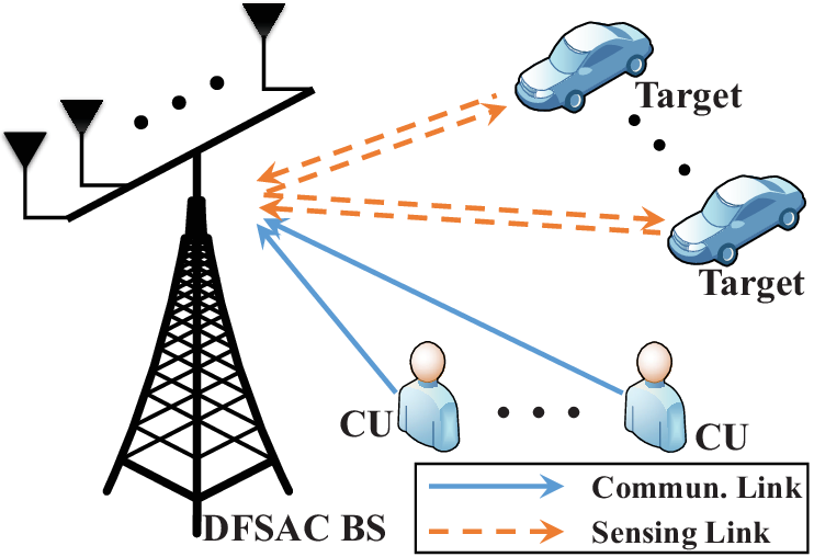
The above arguments imply that the DFSAC BS should work in the full duplex mode. For brevity, we consider that the resultant self-interference is completely eliminated by equipping the BS with two sets of spatially well-separated antennas, i.e., $N$ transmit antennas and $M$ ($M\geq N$) receive antennas. We consider that $M\geq K$ and the CUs communicate with the BS under an uplink NOMA protocol.

The sensing and communication signals are assumed to be perfectly synchronized at the BS by using properly designed synchronization sequences. Consequently, the BS observes the following superposed S&C signal:

The terms appearing in (1) are defined as follows:

• •

  ${\mathbf{S}}=\left[{\mathbf{s}}_{1}\ldots{\mathbf{s}}_{L}\right]\in{\mathbbmss{C}}^{N\times L}$ ($L\geq M$, $L\geq N$) denotes the sensing waveform with $L$ being the pulse length and ${\mathbf{s}}_{l}\in{\mathbbmss{C}}^{N\times 1}$ being the waveform at the $l$th time slot.

• •

  $\mathbf{G}=[\mathbf{g}_{1}\ldots\mathbf{g}_{M}]\in{\mathbbmss{C}}^{N\times M}$ is the target response matrix with $\mathbf{g}_{m}\in{\mathbbmss{C}}^{N\times 1}$ representing the target response from the transmit array to the $m$th receive antenna.

• •

  ${\mathbf{h}}_{k}=[h_{k,1},\ldots,h_{k,M}]^{\mathsf{T}}\in{\mathbbmss{C}}^{M\times 1}$ is the channel vector from CU $k\in{\mathcal{K}}\triangleq\{1,\ldots,K\}$ to BS’s receive antenna array, which is assumed to be known by the BS.

• •

  ${\mathbf{x}}_{k}=\left[x_{k,1},\ldots,x_{k,L}\right]^{\mathsf{H}}\in{\mathbbmss{C}}^{L\times 1}$ denotes the message sent by CU $k\in{\mathcal{K}}$ subject to ${\mathbbmss{E}}\{|x_{k,l}|^{2}\}=p_{\rm{c}}$ with $p_{\rm{c}}$ denoting the communication power.

• •

  ${\mathbf{N}}=\left[{\mathbf{n}}_{1}\ldots{\mathbf{n}}_{L}\right]^{\mathsf{H}}\in{\mathbbmss{C}}^{L\times M}$ is the Gaussian noise matrix containing $LM$ independent and identically distributed (i.i.d.) standard complex Gaussian elements (CGEs).

The target response matrix is modeled as [6, 7]

where $\beta_{q}\sim{\mathcal{CN}}(0,\sigma_{q}^{2})$ is the complex amplitude of the $q$th target with $\sigma_{q}^{2}$ representing the average strength, ${\mathbf{a}}(\theta_{q})\in{\mathbbmss{C}}^{N\times 1}$ and ${\mathbf{b}}(\theta_{q})\in{\mathbbmss{C}}^{M\times 1}$ are the associated transmit and receive array steering vectors, respectively, and $\theta_{q}$ is its direction of arrival. It is worth noting that the target response matrix $\mathbf{G}$ contains all the information about the targets, such as their location and number. Thus, target sensing can be equivalently treated as the estimation of the target response. Assuming that the receive antennas at the BS are widely separated, we have $\mathbf{g}_{m}\sim{\mathcal{CN}}({\mathbf{0}},\mathbf{R})$ for $m\in\{1,\ldots,M\}$ and ${\mathbbmss{E}}\{{\mathbf{g}}_{m}{\mathbf{g}}_{m^{\prime}}^{\mathsf{H}}\}={\mathbf{0}}$ for $m\neq m^{\prime}$. We also assume that the BS knows the correlation matrix ${\mathbf{R}}\in{\mathbbmss{C}}^{N\times N}$, which could be estimated based on multiple previous estimates. The communication channel is characterized by the Rayleigh fading model, which yields $\mathbf{h}_{k}\sim{\mathcal{CN}}({\mathbf{0}},\alpha_{k}\mathbf{I})$ for $k\in{\mathcal{K}}$ and ${\mathbbmss{E}}\{{\mathbf{h}}_{k}{\mathbf{h}}_{k^{\prime}}^{\mathsf{H}}\}={\mathbf{0}}$ for $k\neq k^{\prime}$, where $\alpha_{k}>0$ models the influence of large-scale path loss.

After receiving the superposed signal matrix ${\mathbf{Y}}$, the BS aims to decode the data information contained in the communication signal, $\left\{{\mathbf{x}}_{k}\right\}_{k=1}^{K}$, as well as extracting the environmental information contained in the target response, $\mathbf{G}$. To deal with the ICI and IFI, we propose a two-stage SIC-based framework, in which the inner-stage SIC deals with the ICI while the outer-stage SIC deals with the IFI, as detailed in Fig. 2.

Without loss of generality, we assume that the CUs are arranged in an ascending order, i.e., $\lVert{\mathbf{h}}_{K}\rVert\geq\cdots\geq\lVert{\mathbf{h}}_{1}\rVert$. As Fig. 2 shows, the CUs with better channel conditions are decoded earlier in the inner-stage SIC. As for the outer-stage SIC, we consider two SIC orders. Under the first SIC order, the BS first senses the target response $\mathbf{G}$ by treating the communication signal as interference, and then ${\mathbf{G}}^{\mathsf{H}}{\mathbf{S}}$ is subtracted from $\mathbf{Y}$ with the rest part used for detecting the communication signal. Under the second SIC order, the BS first detects the communication signal $\left\{{\mathbf{x}}_{k}\right\}_{k=1}^{K}$ by treating the sensing signal as interference, and then $\sum\nolimits_{k=1}^{K}{{\mathbf{h}}}_{k}{\mathbf{x}}_{k}^{\mathsf{H}}$ is subtracted from $\mathbf{Y}$ with the rest part used for sensing the target response. Clearly, the first SIC order yields a better communication performance while the second one yields a better sensing performance. Motivated by this, we refer to these two SIC orders as the C-SIC and S-SIC, respectively.

Having established the fundamental model of the two-stage SIC-based framework, we now move to the discussion on the S&C performance achieved by these two SIC orders.

Having investigated the S&C performance achieved by the C-SIC, we now move to the S-SIC.

In the following, we discuss the influence of SIC ordering. Let us first focus on the SR. By comparing (5) with (15), we obtain the following results.

Note that the gap ${\mathcal{E}}_{\rm s}$ is a monotone increasing function of the communication power budget $p_{\rm c}$, which is as expected.

We next consider the sum-CR. By comparing the results in Theorems 2 and 4, we find that the SIC ordering does not influence the diversity order of the sum-CR. As is widely known, the high-SNR OP is determined by the array gain and diversity order [9]. Since the SIC ordering does not influence the diversity order, we can infer that the SIC ordering could affect the array gain. Unfortunately, quantifying the gap with respect to the array gain is challenging, which is left as a potential direction for future work. In the sequel, we compare (9) with (11), which leads to the following results.

After analyzing the S&C performance and discussing the influence of SIC ordering, we next characterize the SR-CR region achieved by NOMA-ISAC.

Notice that $({\mathcal{R}}_{{\rm{s}}}^{\rm{s}},\overline{\mathcal{R}}_{{\rm{c}}}^{\rm{s}})$ and $({\mathcal{R}}_{{\rm{s}}}^{\rm{c}},\overline{\mathcal{R}}_{\rm{c}}^{\rm{c}})$ represent the maximum achievable rate tuples of S-SIC and C-SIC, respectively. Besides, ${\mathcal{R}}_{{\rm{s}}}^{\rm{s}}$ and $\overline{\mathcal{R}}_{{\rm{c}}}^{\rm{c}}$ represent the maximum SR and sum-CR achieved in NOMA-ISAC, respectively. By exploiting the celebrated time-sharing strategy, namely applying the S-SIC with probability $p$, while applying the C-SIC with probability $1-p$, we find that the rate tuple $({\mathcal{R}}_{{\rm{s}}}^{p},\overline{\mathcal{R}}_{{\rm{c}}}^{p})$ is attainable for $p\in[0,1]$, where ${\mathcal{R}}_{{\rm{s}}}^{p}=p{\mathcal{R}}_{{\rm{s}}}^{\rm{s}}+(1-p){\mathcal{R}}_{{\rm{s}}}^{\rm{c}}$ and $\overline{\mathcal{R}}_{{\rm{c}}}^{p}=p\overline{\mathcal{R}}_{{\rm{c}}}^{\rm{s}}+(1-p)\overline{\mathcal{R}}_{{\rm{c}}}^{\rm{c}}$. Let ${\mathcal{R}}^{\rm{s}}$ and ${\mathcal{R}}^{\rm{c}}$ denote the achievable SR and sum ECR, respectively. Then, the rate region achieved by ISAC reads

where $\mathcal{R}_{\rm{c}}^{p}={\mathbbmss{E}}\{\overline{\mathcal{R}}_{\rm{c}}^{p}\}$. By the Sandwich theorem, we get the following results.

Let ${\mathbf{z}}_{m}^{\mathsf{H}}$ and ${\mathbf{n}}_{m}^{\mathsf{H}}$ denote the $m$th row of $\mathbf{Z}$ and ${\mathbf{N}}^{\mathsf{H}}$, respectively. We have ${\mathbf{n}}_{m}\sim{\mathcal{CN}}({\mathbf{0}},{\mathbf{I}})$ and ${\mathbf{z}}_{m}=\sum_{k=1}^{K}h_{k,m}^{*}{\mathbf{x}}_{k}+{\mathbf{n}}_{m}$. It follows that ${\mathbbmss{E}}\{{\mathbf{z}}_{m}\}=0$ and ${\mathbbmss{E}}\{{\mathbf{z}}_{m}{\mathbf{z}}_{m}^{\mathsf{H}}\}={\mathbf{I}}+\sum_{k=1}^{K}{\mathbbmss{E}}\{\lvert h_{k,m}\rvert^{2}\}{\mathbbmss{E}}\{{\mathbf{x}}_{k}{\mathbf{x}}_{k}^{\mathsf{H}}\}=(1+\sum_{k=1}^{K}\alpha_{k}{p_{\rm{c}}}){\mathbf{I}}=\sigma_{\rm{c}}^{2}{\mathbf{I}}$. Moreover, for $m\neq m^{\prime}$, we have ${\mathbbmss{E}}\{{\mathbf{z}}_{m}{\mathbf{z}}_{m^{\prime}}^{\mathsf{H}}\}={\mathbbmss{E}}\{{\mathbf{n}}_{m}{\mathbf{n}}_{m^{\prime}}^{\mathsf{H}}\}+\sum_{k=1}^{K}{\mathbbmss{E}}\{h_{k,m}^{*}h_{k,m^{\prime}}\}{\mathbbmss{E}}\{{\mathbf{x}}_{k}{\mathbf{x}}_{k}^{\mathsf{H}}\}={\mathbf{0}}$. Thus, when $\mathbf{Z}$ is treated as Gaussian noise, it contains $LM$ i.i.d. CGEs each with zero mean and variance $\sigma_{\rm{c}}^{2}$. Using similar steps as those outlined in [7, Appendix C], we can obtain Lemma 1.

As $p_{\rm{c}}\rightarrow\infty$, we have ${\mathcal{R}}_{{\rm{c}}}^{\rm{c}}\approx{\mathbbmss{E}}\{\log_{2}\det(p_{\rm{c}}{{\mathbf{H}}}^{\mathsf{H}}{{\mathbf{H}}})\}$. Note that ${\mathbf{H}}=\overline{\mathbf{H}}\mathsf{diag}\{\sqrt{\alpha_{1}},\ldots,\sqrt{\alpha_{K}}\}$ with $\overline{\mathbf{H}}$ containing $KM$ i.i.d. standard CGEs. It follows that ${\mathbbmss{E}}\{\log_{2}\det(p_{\rm{c}}{{\mathbf{H}}}^{\mathsf{H}}{{\mathbf{H}}})\}={\mathbbmss{E}}\{\log_{2}\det(\overline{{\mathbf{H}}}^{\mathsf{H}}\overline{{\mathbf{H}}})\}+K\log_{2}{p_{\rm c}}+\sum_{k=1}^{K}\log_{2}{\alpha_{k}}$. With the aid of [9, Eq. (C.28)], the final results can be obtained.

Note that ${\mathbbmss{E}}\{{\mathbf{a}}_{l}\}={\mathbbmss{E}}\{{\mathbf{G}}^{\mathsf{H}}{\mathbf{s}}_{l}\}+{\mathbbmss{E}}\{{\mathbf{n}}_{l}\}=0$ and ${\mathbbmss{E}}\{{\mathbf{a}}_{l}{\mathbf{a}}_{l}^{\mathsf{H}}\}={\mathbbmss{E}}\{{\mathbf{G}}^{\mathsf{H}}{\mathbf{s}}_{l}{\mathbf{s}}_{l}^{\mathsf{H}}{\mathbf{G}}\}+{\mathbf{I}}$. Based on the statistics of $\mathbf{G}=[\mathbf{g}_{1}\ldots\mathbf{g}_{M}]$, we have ${\mathbf{g}}_{m}^{\mathsf{H}}{\mathbf{s}}_{l}\sim{\mathcal{CN}}(0,\lvert{\mathbf{s}}_{l}^{\mathsf{H}}{\mathbf{R}}{\mathbf{s}}_{l}\rvert)$. Since ${\mathbf{g}}_{m}$ is independent with ${\mathbf{g}}_{m^{\prime}}$ for $m^{\prime}\neq m$, we have ${\mathbbmss{E}}\{{\mathbf{G}}^{\mathsf{H}}{\mathbf{s}}_{l}{\mathbf{s}}_{l}^{\mathsf{H}}{\mathbf{G}}\}=\lvert{\mathbf{s}}_{l}^{\mathsf{H}}{\mathbf{R}}{\mathbf{s}}_{l}\rvert{\mathbf{I}}$. Thus, when ${\mathbf{a}}_{l}$ is treated as Gaussian noise, it contains $M$ i.i.d. CGEs each with zero mean and variance $\varrho_{l}^{2}=1+|{\mathbf{s}}_{l}^{\mathsf{H}}{\mathbf{R}}{\mathbf{s}}_{l}|$. The final results follow immediately.

References

- [1] F. Liu et al., “Integrated sensing and communications: Towards dual-functional wireless networks for 6G and beyond,” IEEE J. Sel. Areas Commun., vol. 40, no. 6, pp. 1728–1767, Jun. 2022.
- [2] Y. Dong et al., “Joint receiver design for integrated sensing and communications: Is SIC optimal?,” 2022, arXiv:2211.05535.
- [3] M. Liu, M. Yang, and A. Nallanathan, “On the performance of uplink and downlink integrated sensing and communication systems,” in Proc. IEEE Globecom Workshop, 2022, pp. 1236–1241.
- [4] A. R. Chiriyath, B. Paul, G. M. Jacyna, and D. W. Bliss, “Inner bounds on performance of radar and communications co-existence,” IEEE Trans. Signal Process., vol. 64, no. 2, pp. 464–474, Jan. 2016.
- [5] C. Zhang, W. Yi, Y. Liu, and L. Hanzo, “Semi-integrated-sensing-and-communication (Semi-ISaC): From OMA to NOMA,” IEEE Trans. Commun., Early Access, 2023.
- [6] C. Ouyang et al., “On the performance of uplink ISAC systems,” IEEE Commun. Lett., vol. 26, no. 8, pp. 1769–1773, Aug. 2022.
- [7] C. Ouyang et al., “Performance of downlink and uplink integrated sensing and communications (ISAC) systems,” IEEE Wireless Commun. Lett., vol. 11, no. 9, pp. 1850–1854, Sep. 2022.
- [8] B. Hassibi and B. M. Hochwald, “How much training is needed in multiple-antenna wireless links?” IEEE Trans. Inf. Theory, vol. 49, no. 4, pp. 951–963, Apr. 2003.
- [9] R. W. Heath, Jr. and A. Lozano, Foundation MIMO Communication, Cambridge, U.K.: Cambridge Univ. Press, 2018.