openCFS-Data: Data Pre-Post-Processing Tool for openCFS
Abstract
Many numerical simulation tools have been developed and are on the market, but there is still a strong need for appropriate tools capable to simulate multi-field problems, especially in aeroacoustics. Therefore, openCFS provides an open-source framework for implementing partial differential equations using the finite element method. Since 2000, the software has been developed continuously. The result of is openCFS (before 2020 known as CFS++ Coupled Field Simulations written in C++). In this paper, we present for the first time the CFS-Data, the open-source pre-post-processing part of openCFS with a focus on the aeroacoustic source computation (called filters).
Keywords Open Source FEM Software Multiphysics Simulation C++ Acoustics Aero-Acoustics openCFS
1 Introduction
Within this contribution, we concentrate on the openCFS [36] module openCFS-Data. An alternative data processing tool is the recently developed pyCFS-data [48].
When establishing an XML file for CFS-Data, it is fundamental that the pipeline, existing of different CFS-Data filters, is closed. The pipeline has to start with the step value definition and has to be followed by the input filter and end with the output filter. In between, multiple filters can be added, serial or parallel.
Defining Step Value Definition: It is possible to define input data for the time and frequency domain. However, not all filters are capable of processing data in the frequency domain.


Such a serial alignment results in the following structure.
whereas a parallel alignment is set up in the following.
Within the pipeline, different filters can be arranged. The following filter classes are available today:
- •
Interpolation Filters
- •
Conservative Interpolation Filters
- •
Aeroacoustic Source Terms
- •
Synthetic Sources
- •
Data Processing
In this contribution, we discuss the input format, output format and field interpolation possibilities (filters) of CFS-Data in more detail.
2 IO Formats and Definitions
The data processing tool of openCFS offers the option of importing Ensight-files and hdf5-files (hierarchical data format), whereas the export of mesh-based field data is by default based on hdf5, which is the native data format of openCFS. Additionally, reading of meshes (e.g. target mesh for interpolation) in cgns or cdb format is supported. Field data can thereby be defined on the nodes or the cell centroids of a computational grid in the time or the frequency domain.
2.1 Input definition
The first block of the XML-scheme defines the time domain of the input data to be read. The following XML-snippet illustrates a typical setting.
- •
delta: time step size in seconds for data import (”CFS time step”. Thereby, the time step size can be a whole multiple of the time step provided by the input file to read every 2nd, 3rd etc. time step. If for example the input data time step is 1s and the defined ”CFS time step” is 2s, every second time step is read.
- •
startStep: time offset in multiples of the ”CFS time step”.
- •
numSteps: number of time steps to be read.
- •
startTime: offset in seconds according to the input data time values.
- •
deleteOffset: delete the offset resulting from startTime. If set to yes and startStep to zero, the first time value of the output data will be the ”CFS time step” size.
The first time step which is read from the input file is the time step corresponding to the time *startStep* *delta* + *startTime* in seconds. Thereby, the offset resulting from *startTime* can be deleted for the output by enabling the *deleteOffset*-tag. If data is processed in frequency domain, the same tags are used (*startTime* defines the start frequency in this case).
Subsequently, the mesh-based input data is provided by
in case of using the hfd5 format (e.g. *openCFS* simulation file).
*Ensight* data is considered in the XML-scheme by
where in *fileName* the location of the *Ensight* master file (.case or .encas) needs to be provided and the therein defined quantities (e.g. velocity, pressure) need to be defined by *EnsightVarName*. In contrast, the quantities of *hdf5* files are identified automatically by *openCFS*.
2.2 Output definition
The processed field data (*resultQuantity1* and *resultQuantitiy2*) in the following XML-snippet) is exported in the native hdf5-format. Thereby, the filename is defined in the XML scheme and the default file extension CFS can be adapted if required. Furthermore, the default compression level of the hdf5-file of 1 can be modified. Furthermore, external files can be enabled, where the field data of each time/frequency step is written to a separate HDF file and the master file includes the mesh data, further file information, and the links to the external files of each time step. To explore hdf5 files and get an understanding of the structure, *HDFview* is recommended. The results of multiple filters (e.g., *filterID1*, *filterID2* in the following example XML) can be either written to all regions or to specified regions of the output mesh as indicated in the snippet.
It is important if the exported data will be the input of a subsequent *openCFS* simulation, *openCFS* variable names must be used for the declaration of field quantities. Thus, for the acoustic PDE, one of the following names must be chosen.
General acoustic and fluid mechanic quantities:
- •
acouPressure
- •
acouVelocity
- •
acouPotential
- •
acoutIntensity
- •
fluidMechVelocity
- •
meanFluidMechVelocity
- •
fluidMechPressure
- •
fluidMechDensity
- •
fluidMechVorticity
- •
fluidMechGradPressure
Aeroacoustic Source Terms:
- •
acouRhsLoad (general)
- •
acouRhsLoadP (PCWE)
- •
vortexRhsLoad (Vortex Sound Theorie)
- •
acouDivLighthillTensor (Lighthill’s acoustic analogy)
3 Interpolation filters
3.1 Node2Cell
The node to cell interpolation filter takes nodal loads and connects them to the cell center, of the cell defined by those nodes
| (1) |
Thereby, is the load located to the cell, the number of nodes of one element, and the nodal loads. The following example shows this methodology by considering one tetrahedral element:
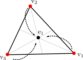
Note it is important that the target mesh is ** not ** the same mesh as the source mesh. Transform source mesh into new, empty mesh by using cfs -g. It is possible to interpolate from a volume onto (curved) surfaces. However, the input data can not be from curved surfaces!
3.2 Cell2Node
The cell to node interpolation filter takes element loads and divides it onto the nodes that build the cell.
| (2) |
The following example shows this methodology by considering one tetrahedral element:
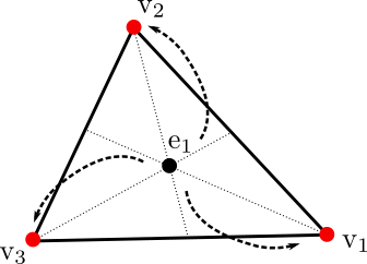
Note it is important that the target mesh is ** not ** the same mesh as the source mesh. Transform source mesh into new, empty mesh by using cfs -g. It is possible to interpolate from a volume onto (curved) surfaces. However, the input data can not be from curved surfaces!
3.3 Nearest Neighbour
The nearest neighbor interpolation of openCFS rests upon the inverse distance weighting (Shepard’s method).

Based on the defined number of neighbours from the source mesh, the nearest neighbours are searched and their distance to the considered node is computed. Based on this distances the weights are computed.
| (3) |
with as being 1.01 times of the maximal distance , and as the interpolation exponent. Shepard stated . Increasing means that values that are further away are taken into account more. Finally, each value of each node that is taken into account is weighted to compute the new value of the considered node
| (4) |
In CFSDat the Nearest Neighbor interpolation is defined in the xml-file as following:
*inputFilterIds* must refer to the id of an input filter which contains the defined ”sourceRegion” and ”quantity”. As target mesh, any compatible file input can be used (see chapter Data Input/Output).
- •
interpolationExponent: Exponent for calculation of interpolation weight function.
- •
globalFactor: Global Factor for scaling the result (usually 1).
- •
numNeighbours: Number of considered Nodes.
3.4 Radial Basis Function Interpolation
This interpolation filter interpolates field data from a source mesh to a target mesh based on radial basis functions (RBFs), where the local Wendland kernel together with a modified Shepard’s method was chosen. Thereby, node-based data can be interpolated either to the cell centroids or the nodes of the source mesh, whereas element-based data can currently only be interpolated to the cell-centroids. The theoretical background of the implemented interpolation scheme is published in [23].
Like for all interpolation filters, the input and output quantitiy, the source and target regions, and the target mesh have to be defined within the xml-scheme. By using the optional tag *noSlipWall*, the output quantity of the nodes on the specified wall region (boundary surface) are set to zero. This tag is intended to consider no-slip-walls for the interpolation of the flow velocity but can theoretically also be used for other quantities.
The field data is interpolated to the nodes of the target mesh by default. By setting *useElemAsTarget* *true*, the field data is interpolated to the cell centroids of the target mesh. The tag *interpolationExponent* handles the locality of the approximation on the target mesh and is considered within the weight function (for details see [@schoder2020c]). The larger it is, the more local the approach making it less accurate but capable of resolving stronger gradients. Furthermore, *globalFactor* allows a scaling of the output by the defined factor.
The number of neighbour points (*numNeighbours*) and influence points (*numNeighbours_weight*) are by default set to and , which is a compromise of accuracy and numerical efficiency for 2D and 3D interpolations. The interopolation result can be enhanced by tuning these parameters specifically for the involved source and target mesh. By setting the tag *useCGAL4RBF* to *true*, the nearest neighbor search will be carried out be by CGAL, which requires the *CGAL 3.3* build (cmake flag must be set in the cmake build properties(../Installation/linuxinstall/)).
3.5 Finite Element (FE) based Interpolation
This filter (beta version) is currently under development and not all functionality is fully tested. A preliminary documentation can be found online in the CFS repository.
4 Conservative source integration
The conservative interpolation computes the Right-hand Side force of a partial differential equation
| (5) |
using first order nodal FEM to solve the system of equations. If you would like to use the conservative filters for higher order FEM, please contact the authors. [40] covers the theory of the implemented conservative interpolation filters. For further development and future publications on the topic, we are happy to collaborate with you.
Pipeline setup
During the simulation setup, we will discuss how the variables inside the publication relate to the XML-scheme of the simulation setup. Having this knowledge, it should be able for you to start your simulation using conservative interpolators. CGNS or ENSIGHT input data is supported.
There are two variants implemented and their application limits are discussed in [40]. The cell centroid interpolator is defined by the type variable
based on figure 6, the interpolation is carried out.

The cut volume cell interpolator is defined by the type variable
based on figure 7, the interpolation is carried out.

5 Field derivatives
5.1 Gradient
The gradient operator calculates the gradient of a scalar source quantity .
The derivative is performed on radial basis functions [23]. The filter is defined as following in the CFSdat xml input:
In *RBF_Settings*, the following (optional and mandatory) attributes may be adjusted:
- •
epsilonScaling (mandatory): Controls the ”smoothness” of the basis function. The smoother the Gauss-like surface is, the better the results will be BUT only until a certain number, when the matrix becomes so ill-conditioned, which will either result in an exception or very bad results. Typical values 0.1
- •
betaScaling: Slope of the linear term that was added to the radial basic functions
- •
kScaling: constant term that was added to the radial basic functions
- •
logEps: Console output of [minimal distance, maximal distance, optimized epsilon]. If you run into convergence troubles of the matrix inversion one can activate this. It is only recommended for investigating the quality of the derivative, because it produces a lot of console output.
5.2 Divergence
The divergence operator calculates the divergence of a source vector . The filter is defined as following in the CFSdat xml input:
5.3 Curl
The curl operator calculates the curl of a source vector . The filter is defined as following in the CFSdat xml input:
6 Aeroacoustic source terms
6.1 Lamb Vector
The Lamb Vector filter computes the Lamb vector based on the velocity , vorticity and the density .
| (6) |
with vorticity as
| (7) |
However, it is possible to compute the Lamb vector only based on the velocity, or on the velocity and the vorticity. If only the velocity is defined, the vorticity is computed internally.
- •
The epsilonScaling Parameter scales the radial basis functions used for computing spatial derivatives [23]. It controls the “smoothness” of the basis function. The smoother the gauss-like surface is, the better the results will be, BUT only until a certain number, when the matrix becomes too ill-conditioned, which will result in very bad results. Typical values: 1e-1 - 1e-4.
- •
The kScaling parameter is an optional parameter and defines a constant term that is added to the radial basic function.
- •
The betaScaling parameter defines the slope of a linear term that is added to the radial basis function.
- •
The logEps Parameter enables a detailes console output (minimal distance, maximal distance, optimized parameters). Therefore, it should only be used if the spatial derivatives are investigated, because it totally spams the console
6.2 Lighthill Source Term
The Lighthill source term filter computes aeroacoustic source terms based on Lighthill’s analogy for incompressible flows. Therefore, first the Lighthill source term vector is computed
| (8) |
with as velocity, and as Lamb vector, and as the Lighthill stress tensor. Finally, as actual source term, the divergence of the source term vector is computed and established as outputQuantity.
| (9) |
It is possible to compute the Lighthill source term only based on the velocity, or on the velocity and the vorticity. If only the velocity is defined, the vorticity is computed internally and the parameters are the same as for the Lamb vector.
6.3 Lighthill Source Term Vector
The Lighthill source term vector computes a vector corresponding with the , where denotes the Lighthill stress tensor, for incompressible flows.
It is possible to compute the Lighthill source term vector only based on the velocity, or on the velocity and the vorticity. If only the velocity is defined, the vorticity is computed internally and the parameters are the same as for the Lamb vector.
6.4 Time Derivative (Simplified PCWE Source Term)
For low flow velocities, convective effects may be neglected for the PCWE, and the resulting source term simplifies to just the time derivative of the incompressible pressure . This is the reason the time derivative filter is placed in the section *Aeroacoustic Source Terms*. Of course, the filter can be applied to a different quantity, of which a time derivative is required, as well.
The time derivative of the desired quantity is computed by a smooth noise-robust differentiator, which suppresses high frequencies and is precise on low frequencies, according to this website. For an efficient and robust calculation the order of the differentiator is set to and the time derivative is calculated by
| (10) |
where the index of defines the time step relative to the time step of which the derivative is calculated and is the time step size. The computation only requires the definition of the input quantity (*inputQuantity*-tag) and the desired name of the output quantity (*outputQuantity*-tag) as indicated below.
7 Applications
In a number of different publications, the details on the module [21, 27, 20] are presented, and applied it to special aeroacoustic source models [6, 34, 23, 27, 47, 24, 26, 11], and special wave equation models [9, 41] are available. Since 2016, the software provided solutions for challenges in acoustical engineering and medicine. Car frame noise [1, 3, 29, 47, 16], fan noise [22, 43, 8, 7, 40, 44, 45, 19, 37] noise emissions of the turbocharger compressor [5, 10, 4], HVAC systems were computed. For post-processing, the fluid field was decomposed into a longitudinal and transversal processes [33, 32, 25, 31]. Furthermore, the human phonation process is studied in detail [39, 46, 49, 30, 2, 13, 15, 35, 14, 28, 42, 12]. The conservative source term interpolation is used in many aeroacoustic workflows including the FEM-assembly of aeroacoustic source terms of the aeroacoustic wave equation based on Pierce operator [18, 38, 26] and the compressible perturbed convective wave equation [41, 17].
8 Acknowledge
We would like to acknowledge the authors of openCFS.
References
- [1] (2020) A generic testbody for low-frequency aeroacoustic buffeting. Technical report SAE Technical Paper. Cited by: §7.
- [2] (2021) 3D-fv-fe aeroacoustic larynx model for investigation of functional based voice disorders. Frontiers in physiology 12, pp. 616985. Cited by: §7.
- [3] (2021) Simulationen von strömungsakustik in rotierenden bauteilen zur entwicklung von antriebskonzepten der autos der zukunft. e & i Elektrotechnik und Informationstechnik 138 (3), pp. 212–218. Cited by: §7.
- [4] (2020) The influences of spatial and temporal discretization in flow simulation on lighthill’s aeroacoustic source terms applied to a turbocharger. In AIAA AVIATION 2020 FORUM, pp. 2546. Cited by: §7.
- [5] (2022) Applicability of two hybrid sound prediction methods for assessing in-duct sound absorbers of turbocharger compressors. Acta Acustica 6, pp. 37. Cited by: §7.
- [6] (2010) Numerical Simulation of Flow-Induced Noise Using LES/SAS and Lighthill’s Acoustics Analogy. International Journal for Numerical Methods in Fluids 63 (9), pp. 1103–1122. Cited by: §7.
- [7] (2016) Modeling and Finite Element Formulation for Acoustic Problems Including Rotating Domains. AIAA Journal. Cited by: §7.
- [8] (2017) Computational Acoustics. CISM International Centre for Mechanical Sciences, Springer International Publishing. External Links: ISBN 9783319590387 Cited by: §7.
- [9] (2018) Nonconforming finite elements based on nitsche-type mortaring for inhomogeneous wave equation. Journal of theoretical and computational acoustics 26 (03), pp. 1850028. Cited by: §7.
- [10] (2020) Modelling and numerical simulation of the noise generated by automotive turbocharger compressor. Technical report SAE Technical Paper. Cited by: §7.
- [11] (2021) Physical models for flow: acoustic interaction. In Waves in Flows, pp. 265–353. Cited by: §7.
- [12] (2022) Machine-learning applied to classify flow-induced sound parameters from simulated human voice. arXiv preprint arXiv:2207.09265. Cited by: §7.
- [13] (2021) Impact of the sub-grid scale turbulence model in aeroacoustic simulation of human voice. Applied Sciences 11 (4), pp. 1970. Cited by: §7.
- [14] (2023) Anisotropic minimum dissipation subgrid-scale model in hybrid aeroacoustic simulations of human phonation. arXiv preprint arXiv:2301.00606. Cited by: §7.
- [15] (2021) Efficient numerical simulation of the human voice. e & i Elektrotechnik und Informationstechnik 138 (3), pp. 219–228. Cited by: §7.
- [16] (2022) Aeroacoustic formulations for confined flows based on incompressible flow data. Acta Acustica 6, pp. 45. Cited by: §7.
- [17] (2025) Perturbed convective wave equation for low-to-medium mach number subsonic flows. Journal of Sound and Vibration, pp. 119549. Cited by: §7.
- [18] (2024) Aeroacoustic source potential based on poisson’s equation. AIAA Journal 62 (7), pp. 2772–2782. Cited by: §7.
- [19] (2022) Dataset fan-01: revisiting the eaa benchmark for a low-pressure axial fan. arXiv preprint arXiv:2211.12014. Cited by: §7.
- [20] (2020) Conservative interpolation of aeroacoustic sources in a hybrid workflow applied to fan. arXiv preprint arXiv:2009.02341. Cited by: §7.
- [21] (2018) Aeroacoustic analogies based on compressible flow data. Ph.D. Thesis, Wien. Cited by: §7.
- [22] (2020) Computational aeroacoustics of the eaa benchmark case of an axial fan. Acta Acustica 4 (5), pp. 22. Cited by: §7.
- [23] (2020) Radial basis function interpolation for computational aeroacoustics. In AIAA AVIATION 2020 FORUM, pp. 2511. Cited by: §3.4, §5.1, 1st item, §7.
- [24] (2019) Conservative source term interpolation for hybrid aeroacoustic computations. In 25th AIAA/CEAS aeroacoustics conference, pp. 2538. Cited by: §7.
- [25] (2019) Helmholtz’s decomposition applied to aeroacoustics. In 25th AIAA/CEAS Aeroacoustics Conference, Cited by: §7.
- [26] (2022) Aeroacoustic wave equation based on pierce’s operator applied to the sound generated by a mixing layer. In 28th AIAA/CEAS Aeroacoustics 2022 Conference, pp. 2896. Cited by: §7.
- [27] (2019) Hybrid aeroacoustic computations: state of art and new achievements. Journal of Theoretical and Computational Acoustics 27 (04), pp. 1950020. Cited by: §7.
- [28] (2022) Error detection and filtering of incompressible flow simulations for aeroacoustic predictions of human voice. The Journal of the Acoustical Society of America 152 (3), pp. 1425–1436. Cited by: §7.
- [29] (2020) Numerical investigation of a deep cavity with an overhanging lip considering aeroacoustic feedback mechanism. arXiv preprint arXiv:2006.03279. Cited by: §7.
- [30] (2021) Aeroacoustic sound source characterization of the human voice production-perturbed convective wave equation. Applied Sciences 11 (6), pp. 2614. Cited by: §7.
- [31] (2022) Post-processing subsonic flows using physics-informed neural networks. In 2023 AIAA AVIATION Forum, Cited by: §7.
- [32] (2020) Helmholtz’s decomposition for compressible flows and its application to computational aeroacoustics. SN Partial Differ. Equ. Appl., pp. 1–20. Cited by: §7.
- [33] (2020) Postprocessing of direct aeroacoustic simulations using helmholtz decomposition. AIAA Journal, pp. 1–9. Cited by: §7.
- [34] (2020) Aeroacoustic source term computation based on radial basis functions. International Journal for Numerical Methods in Engineering 121 (9), pp. 2051–2067. Cited by: §7.
- [35] (2022) Learning expertise actively to model domain knowledge (lead) with application to human phonation. arXiv. Cited by: §7.
- [36] (2022) OpenCFS: open source finite element software for coupled field simulation–part acoustics. arXiv preprint arXiv:2207.04443. Cited by: §1.
- [37] (2022) Quantification of the acoustic emissions of an electric ducted fan unit. In 2022 Delft International Conference on Urban Air-Mobility: DICUAM 2022, Cited by: §7.
- [38] (2023) Acoustic modeling using the aeroacoustic wave equation based on pierce’s operator. AIAA Journal 61 (9), pp. 4008–4017. Cited by: §7.
- [39] (2020) Hybrid aeroacoustic approach for the efficient numerical simulation of human phonation. The Journal of the Acoustical Society of America 147 (2), pp. 1179–1194. Cited by: §7.
- [40] (2021) Application limits of conservative source interpolation methods using a low mach number hybrid aeroacoustic workflow. Journal of Theoretical and Computational Acoustics 29 (01), pp. 2050032. Cited by: §4, §4, §7.
- [41] (2022) CPCWE–perturbed convective wave equation based on compressible flows. arXiv preprint arXiv:2209.11410. Cited by: §7.
- [42] (2022) PCWE for fsai–derivation of scalar wave equations for fluid-structure-acoustics interaction of low mach number flows. arXiv preprint arXiv:2211.07490. Cited by: §7.
- [43] (2018) Source formulations and boundary treatments for lighthill’s analogy applied to incompressible flows. AIAA Journal 56 (7), pp. 2769–2781. Cited by: §7.
- [44] (2022) Machine-learning clustering methods applied to detection of noise sources in low-speed axial fan. In 2022 Turbomachinery Technical Conference & Exposition: ASME Turbo Expo 2022, Cited by: §7.
- [45] (2023) Machine-learning clustering methods applied to detection of noise sources in low-speed axial fan. Journal of Engineering for Gas Turbines and Power 145 (3), pp. 031020. Cited by: §7.
- [46] (2019) On the application of acoustic analogies in the numerical simulation of human phonation process. Flow, Turbulence and Combustion 102 (1), pp. 129–143. Cited by: §7.
- [47] (2019) Numerical investigation of the resonance behavior of flow-excited helmholtz resonators. PAMM 19 (1), pp. e201900033. Cited by: §7.
- [48] (2024) PyCFS-data: data processing framework in python for opencfs. arXiv preprint arXiv:2405.03437. Cited by: §1.
- [49] (2016) Flow and acoustic effects in the larynx for varying geometries. Acta Acustica united with Acustica 102 (2), pp. 257–267. Cited by: §7.