On the relationship between multivariate splines
and infinitely-wide neural networks

Francis Bach Affiliation: Inria, Ecole Normale Supérieure Affiliation: PSL Research University Email: francis.bach@inria.fr

August 11, 2026

Abstract

We consider multivariate splines and show that they have a random feature expansion as infinitely wide neural networks with one-hidden layer and a homogeneous activation function which is the power of the rectified linear unit. We show that the associated function space is a Sobolev space on a Euclidean ball, with an explicit bound on the norms of derivatives. This link provides a new random feature expansion for multivariate splines that allow efficient algorithms. This random feature expansion is numerically better behaved than usual random Fourier features, both in theory and practice. In particular, in dimension one, we compare the associated leverage scores to compare the two random expansions and show a better scaling for the neural network expansion.

1 Introduction

Multivariate non-parametric regression can be approached from a variety of methods: decision trees, local averaging methods such as Nadaraya-Watson estimation or $k$ -nearest-neighbor regression, neural networks, and methods based on positive definite kernels such as smoothing splines, kriging, and kernel ridge regression (see, e.g., [1, 2, 3]).

In this paper, we build on the following known relationship between kernel-based methods and infinitely-wide neural networks [4, 5]. We consider an activation function $\sigma:\mathbb{{R}}\to\mathbb{{R}}$ , and a one-hidden-layer neural network model on $\mathbb{{R}}^{d}$ of the form

f(x)=\sum_{j=1}^{m}\eta_{j}\sigma(w_{j}^{\top}x+b_{j}),

where $\eta_{j}\in\mathbb{{R}}$ , $(w_{j},b_{j})\in\mathbb{{R}}^{d+1}$ , for $j=1,\dots,m$ . When an $\ell_{2}$ -regularization is added to the objective function which is used to fit the model, this is equivalent to using a kernel-based method with positive-definite kernel

\hat{k}(x,y)=\frac{1}{m}\sum_{j=1}^{m}\sigma(w_{j}^{\top}x+b_{j})\sigma(w_{j}^{\top}y+b_{j}).

(1)

See, e.g., [6] for an introduction to kernel methods. If the $m$ input weights $(w_{j},b_{j})\in\mathbb{{R}}^{d+1}$ are sampled independently and identically distributed, when $m$ tends to infinity, by the law of large numbers, $\hat{k}(x,y)$ tends to the equivalent kernel

k(x,y)={\mathbb{E}}_{(w,b)}\big[\sigma(w^{\top}x+b)\sigma(w^{\top}y+b)\big].

(2)

This equivalence between infinitely wide neural networks and kernel methods has already been used in several ways:

•

Given a known kernel $k$ which can be expressed as an expectation as in Eq. (2), we can use the approximate kernel $\hat{k}$ as in Eq. (1), and its explicit random features to derive efficient algorithms [5, 7]: with $n$ observations, we can circumvent the computation of the $n\times n$ kernel matrix by computing the $m$ -dimensional feature vector for each of the $n$ observations, which is advantageous when $m<n$ .
•

Given a known neural network architecture, they allow the study of the regularization properties of using over-parameterized models, that is, with the number of hidden neurons going to infinity [8].

In this paper, we make the following contributions, that contribute to the two ways mentioned above of relating kernels and neural networks:

•

We consider multivariate splines [9, 10], with kernels proportional to $\|x-y\|_{2}^{2\alpha+1}$ , for $\alpha\in\mathbb{N}$ (where $\|\cdot\|_{2}$ denotes the standard Euclidean norm), and show that they have a random feature expansion as infinitely wide neural networks with one-hidden layer and a homogeneous activation function which is the $\alpha$ -th power of the “rectified linear unit” [11]. This extends the earlier work of [8], which proved this link for $\alpha=0$ (step activation function).
•

We show that the associated function space is a Sobolev space with order $s=\frac{d+1}{2}+\alpha$ , with an explicit dependence between the norms.
•

This link provides a new random feature expansion for multivariate splines that allow efficient algorithms. This random feature expansion numerically behaves better than usual random Fourier features, both in theory and practice. In particular, in dimension one, we compare the associated leverage scores [12] to compare the two random expansions. This also provides a more efficient alternative to random Fourier feature expansion for all Matérn kernels [23, page 84].

2 From one-hidden layer neural networks to positive-definite kernels

We consider the Euclidean ball ${\mathbb{B}}^{d}(R)$ of center $0$ and radius $R$ in $\mathbb{{R}}^{d}$ , for $R>0$ , and consider the estimation of real-valued functions on ${\mathbb{B}}^{d}(R)$ .

For $\alpha\in\mathbb{N}$ , we consider activation functions $\sigma$ of the form $\sigma(u)=(u_{+})^{\alpha}=\max\{u,0\}^{\alpha}$ , that is, $\sigma(u)=0$ for $u\leqslant 0$ , and $\sigma(u)=u^{\alpha}$ for $u>0$ , with the usual convention that $u^{0}=1$ if $u>0$ , with a particular focus on $\alpha\in\{0,1\}$ . For $\alpha=0$ , we recover the step-function $\sigma(u)=1_{u>0}$ , and for $\alpha=1$ the rectified linear unit $\sigma(u)=u_{+}$ .

We consider randomly distributed weights $(w,b)\in\mathbb{{R}}^{d+1}$ , and the positive definite kernel

k(x,y)={\mathbb{E}}_{(w,b)}\big[\sigma(w^{\top}x+b)\sigma(w^{\top}y+b)\big].

Since we use homogeneous activation functions, we can normalize weights $(w,b)$ so that they have compact supports. Several normalizations and distributions can be used to obtain closed-form formulas.

Full spherical symmetry in $\mathbb{{R}}^{d+1}$ .

The first normalization is to write

w^{\top}x+b={w\choose b/R}^{\top}{x\choose R},

and let ${w\choose b/R}$ be rotationally invariant, for example, be uniformly distributed on the unit $\ell_{2}$ -sphere in dimension $\mathbb{{R}}^{d+1}$ . This leads to closed-form formulas [13, 14] for the corresponding kernel $\tilde{k}^{(\alpha)}_{d}$ , with $\displaystyle\cos\varphi=\frac{x^{\top}y+R^{2}}{(\|x\|_{2}^{2}+R^{2})^{1/2}(\|y\|_{2}^{2}+R^{2})^{1/2}}\geqslant 0$ (so that $\varphi\in[0,\pi/2]$ ), leading to for small values of $\alpha$ :

$\displaystyle\tilde{k}^{(0)}_{d}(x,y)$	$\displaystyle=$	$\displaystyle\frac{1}{2\pi}(\pi-\varphi)$
$\displaystyle\tilde{k}^{(1)}_{d}(x,y)$	$\displaystyle=$	$\displaystyle\frac{1}{2\pi(d+1)}(\\|x\\|_{2}^{2}+R^{2})^{1/2}(\\|y\\|_{2}^{2}+R^{2})^{1/2}\times\big[\sin\varphi+(\pi-\varphi)\cos\varphi\big]$
$\displaystyle\tilde{k}^{(2)}_{d}(x,y)$	$\displaystyle=$	$\displaystyle\frac{1}{2\pi(d+1)(d+3)}(\\|x\\|_{2}^{2}+R^{2})(\\|y\\|_{2}^{2}+R^{2})\times\big[3\sin\varphi\cos\varphi+(\pi-\varphi)(1+2\cos^{2}\varphi)\big].$

More generally (see [13]), we have:

\tilde{k}^{(\alpha)}_{d}(x,y)=\frac{1}{2\pi(d+1)(d+3)\cdots(d+2\alpha-1)}(\|x\|_{2}^{2}+R^{2})^{\alpha/2}(\|y\|_{2}^{2}+R^{2})^{\alpha/2}\times J_{\alpha}(\varphi),

with $J_{\alpha}(\varphi)=(-1)^{\alpha}(\sin\varphi)^{2\alpha+1}\Big(\frac{1}{\sin\varphi}\frac{d}{d\varphi}\Big)^{\alpha}\Big(\frac{\pi-\varphi}{\sin\varphi}\Big)$ , which is of the form $P_{\alpha}(\cos\varphi,\sin\varphi)+Q_{\alpha}(\cos\varphi,\sin\varphi)(\pi-\varphi)$ for $P_{\alpha}$ and $Q_{\alpha}$ polynomials of degree less than $\alpha$ .

Regularization properties.

The associated space of functions can be described through spherical harmonics in ambient dimension $d+1$ , as, e.g., described in [15, 14], through the use of the Laplacian on the hyper-sphere. This requires, however, strong knowledge of spherical harmonics and is not easy to relate to classical notions of derivatives in $\mathbb{{R}}^{d}$ . Note that Hermite polynomials can be used as well [16]. Overall we obtain the Sobolev space with degree $s=\frac{d+1}{2}+\alpha$ over ${\mathbb{B}}^{d}(R)$ , but with a non-explicit expression in terms of derivatives.

In this paper, we consider another normalization with easier interpretations and links with existing kernels from the statistical literature. This is done using only a spherical symmetry on $w\in\mathbb{{R}}^{d}$ .

Partial spherical symmetry (in $\mathbb{{R}}^{d})$ .

We can instead choose to have ${w\choose b/R}$ uniformly distributed on the product $\mathbb{S}^{d-1}\times[-1,1]$ where $\mathbb{S}^{d-1}\subset\mathbb{{R}}^{d}$ is the unit $\ell_{2}$ -sphere, following [8] that introduced this normalization for $\alpha=0$ . This corresponds to $w$ uniform on the sphere $\mathbb{S}^{d-1}$ and $b$ uniform on $[-R,R]$ .

The main goal of this paper is to provide closed-form formulas for the kernel as well as to study the regularization properties. We will start in dimension one ( $d=1$ ) and extend to all dimensions in later sections.

We thus define the positive-definite kernel:

k_{d}^{(\alpha)}(x,y)={\mathbb{E}}_{(w,b)}\big[(w^{\top}x+b)_{+}^{\alpha}(w^{\top}y+b)_{+}^{\alpha}\big],

where $(w,b)$ is uniform on ${\mathbb{S}}^{d-1}\times[-R,R]$ .

3 Kernels on the interval $[-R,R]$ ( $d=1$ )

We first consider the kernel for $d=1$ , where $w\in\{-1,1\}$ , for which we have, by a change of variable $b\to-b$ :

	$\displaystyle k_{1}^{(\alpha)}(x,y)$	$\displaystyle=$	$\displaystyle\frac{1}{4R}\int_{-R}^{R}(x+b)_{+}^{\alpha}(y+b)^{\alpha}_{+}db+\frac{1}{4R}\int_{-R}^{R}(-x+b)_{+}^{\alpha}(-y+b)^{\alpha}_{+}db$
		$\displaystyle=$	$\displaystyle\frac{1}{4R}\int_{-R}^{R}(x-b)_{+}^{\alpha}(y-b)^{\alpha}_{+}db+\frac{1}{4R}\int_{-R}^{R}(b-x)_{+}^{\alpha}(b-y)^{\alpha}_{+}db.$

3.1 Closed-form formulas

We first consider the case $\alpha=0$ and then generalize from it. We have for $\alpha=0$ , by direct integration:

	$\displaystyle k_{1}^{(0)}(x,y)$	$\displaystyle=$	$\displaystyle\frac{1}{4R}\int_{-R}^{\min\{x,y\}}db+\frac{1}{4R}\int_{\max\{x,y\}}^{R}db=\frac{1}{2}-\frac{1}{4R}\big[\max\{x,y\}-\min\{x,y\}\big]$
		$\displaystyle=$	$\displaystyle\frac{1}{2}-\frac{1}{4R}\|x-y\|.$

A more tedious direct computation gives the expression for other small values of $\alpha$ , as:

	$\displaystyle k_{1}^{(1)}(x,y)$	$\displaystyle=$	$\displaystyle\frac{R^{2}}{6}+\frac{1}{2}xy+\frac{1}{24R}\|x-y\|^{3}$
	$\displaystyle k_{1}^{(2)}(x,y)$	$\displaystyle=$	$\displaystyle\frac{R^{4}}{10}+\frac{2R^{2}xy}{3}+\frac{R^{2}}{6}(x^{2}+y^{2})+\frac{1}{2}x^{2}y^{2}-\frac{1}{120R}\|x-y\|^{5}.$

This can be extended to all values in $\alpha$ in the following proposition, shown in Appendix B.1. Note that in one dimension, [17] already made the connection between cubic splines and infinitely-wide neural networks.

Proposition 1 (Closed-form formula for $d=1$ )

Let $\alpha\in\mathbb{N}$ , we have, for $(w,b)$ uniformly distributed on the product $\{-1,1\}\times[-R,R]$ ,

k_{1}^{(\alpha)}(x,y)={\mathbb{E}}_{(w,b)}\big[(w^{\top}x+b)_{+}^{\alpha}(w^{\top}y+b)_{+}^{\alpha}\big]=P^{(\alpha)}_{1}(x^{2},y^{2},xy)+\frac{1}{R}c^{(\alpha)}_{1}|x-y|^{2\alpha+1},

where $P^{(\alpha)}_{1}$ is a polynomial of degree $\alpha$ , such that $k_{1}^{(\alpha),({\rm pol})}(x,y)=P^{(\alpha)}_{1}(x^{2},y^{2},xy)$ is a positive-definite kernel, and $\displaystyle c^{(\alpha)}_{1}=\frac{(-1)^{\alpha+1}}{4}\frac{(\alpha!)^{2}}{(2\alpha+1)!}$ .

Moreover, as shown in Appendix B.1, we have a special form of polynomial kernel $k_{1}^{(\alpha),({\rm pol})}(x,y)=P^{(\alpha)}_{1}(x^{2},y^{2},xy)$ , as:

$\displaystyle k_{1}^{(\alpha),({\rm pol})}(x,y)$	$\displaystyle=$	$\displaystyle\frac{1}{4R}\int_{-R}^{R}(x-b)^{\alpha}(y-b)^{\alpha}db,\ \mbox{ which can be expressed as}$
$\displaystyle k_{1}^{(\alpha),({\rm pol})}(x,y)$	$\displaystyle=$	$\displaystyle\frac{1}{2R}\sum_{i,j=0}^{\alpha}1_{i+j\ {\rm even}}\cdot{\alpha\choose i}{\alpha\choose j}{x^{i}y^{j}}\frac{R^{2\alpha+1-i-j}}{2\alpha+1-i-j}$	(3)
	$\displaystyle=$	$\displaystyle\frac{1}{2}\sum_{s=0}^{\alpha}\frac{R^{2\alpha-2s}}{2\alpha+1-2s}\sum_{i,j=0}^{\alpha}1_{i+j=2s}\cdot{\alpha\choose i}{\alpha\choose j}{x^{i}y^{j}}.$	(3)

Note that the term for $s=0$ , is $\frac{R^{2\alpha}}{2(2\alpha+1)}$ , while for $\alpha>0$ , the term corresponding to $s=1$ is equal to $\frac{\alpha^{2}R^{2(\alpha-1)}}{2(2\alpha-1)}xy$ . In all cases, it can be computed in time at most $O(\alpha^{2})$ . Moreover, the corresponding feature space leads to all polynomials of degree less than $\alpha$ (see proof in Appendix B.3). This result will be directly extended to dimensions $d$ greater than one in Prop. 3.

3.2 Corresponding norm

All positive-definite kernels define a Hilbert space of real-valued functions on ${\mathbb{B}}^{d}(R)$ with a particular norm. For kernels that can be expressed as expectations, this norm $\Omega_{1}^{(\alpha)}$ is equal to [18, 14]:

	$\displaystyle\Omega_{1}^{(\alpha)}(f)^{2}$	$\displaystyle=$	$\displaystyle\inf_{\eta_{\pm}:[-R,R]\to\mathbb{{R}}}\frac{1}{4R}\int_{-R}^{R}\big[\eta_{+}(b)^{2}+\eta_{-}(b)^{2}\big]db$
			$\displaystyle\mbox{ such that }\forall x\in[-R,R],f(x)=\frac{1}{4R}\int_{-R}^{R}\big[\eta_{+}(b)(x-b)_{+}^{\alpha}+\eta_{-}(b)(b-x)_{+}^{\alpha}\big]db,$

where the infimum is taken over square-integrable functions $\eta_{+}$ and $\eta_{-}$ .

Special case $\alpha=0$ .

For $f$ continuously differentiable, we can use and average the two simple representations:

f(x)=f(-R)+\int_{-R}^{x}f^{\prime}(b)(x-b)_{+}^{0}db=f(R)-\int_{-R}^{R}f^{\prime}(b)(b-x)_{+}^{0}db,

to get $\displaystyle f(x)=\frac{1}{2}[f(R)+f(-R)]+2R\int_{-R}^{R}f^{\prime}(b)(x-b)_{+}^{0}\frac{db}{4R}-2R\int_{-R}^{R}f^{\prime}(b)(b-x)_{+}^{0}\frac{db}{4R}.$ The constant function equal to $1/2$ on $[-R,R]$ can be represented as:

\int_{-R}^{R}(x-b)_{+}^{0}\frac{db}{4R}+\int_{-R}^{R}(b-x)_{+}^{0}\frac{db}{4R}.

We can thus take: $\eta_{+}(b)=2Rf^{\prime}(b)+[f(R)+f(-R)]$ and $\eta_{+}(b)=-2Rf^{\prime}(b)+[f(R)+f(-R)]$ .

This leads to the squared norm $\Omega_{1}^{(0)}(f)^{2}$ less than (since the cross-terms cancel):

2R\int_{-R}^{R}f^{\prime}(x)^{2}dx+\big[f(-R)+f(R)\big]^{2}.

In particular, the norm is finite as soon as the quantity above is well-defined, that is, $f^{\prime}$ square integrable. To show that this is indeed the correct norm, we simply need to check that our representation is optimal, which is shown below for all $\alpha$ ’s (see Prop. 2). Thus

\Omega_{1}^{(0)}(f)^{2}=2R\int_{-R}^{R}f^{\prime}(x)^{2}dx+\big[f(-R)+f(R)\big]^{2}.

General case $\alpha\geqslant 0$ .

To obtain the norm, we can notice that continuous expansions with functions $(x-b)_{+}^{\alpha}$ are exactly obtained from Taylor expansions with integral remainders, which apply to functions defined on $[-R,R]$ with $\alpha+1$ continuous derivatives:

f(x)=\sum_{i=0}^{\alpha}\frac{f^{(i)}(-R)}{i!}(x+R)^{i}+\int_{-R}^{R}\frac{f^{(\alpha+1)}(b)}{\alpha!}(x-b)_{+}^{\alpha}db.

Ignoring the boundary conditions, we see that $\eta_{+}(b)$ should be related to $\frac{1}{\alpha!}f^{(\alpha+1)}(b)$ , and that the RKHS norm should include the integral $\displaystyle\int_{R}^{R}f^{(\alpha+1)}(x)^{2}dx$ . The following proposition makes this explicit (see proof in Appendix B.2).

Proposition 2 (RKHS norm for $d=1$ )

The RKHS norm on functions on $[-R,R]$ associated to the kernel $k_{1}^{(\alpha)}$ is equal to:

\Omega_{1}^{(\alpha)}(f)^{2}=\frac{2R}{\alpha!^{2}}\int_{-R}^{R}f^{(\alpha+1)}(x)^{2}dx+\Theta^{(\alpha)}\big[f^{(0)}(-R),f^{(0)}(R),\dots,f^{(\alpha)}(-R),f^{(\alpha)}(R)\big],

where $\Theta^{(\alpha)}$ is non-negative quadratic form.

For example, for $\alpha=1$ , we get:

\displaystyle\Omega_{1}^{(1)}(f)^{2}

\displaystyle=

\displaystyle 2R\int_{-R}^{R}f^{\prime\prime}(x)^{2}dx+\big[f^{\prime}(R)+f^{\prime}(-R)\big]^{2}+\frac{3}{2R^{2}}\big[f(-R)+f(R)-Rf^{\prime}(R)+Rf^{\prime}(-R)\big]^{2}.

Equivalence to classical Sobolev norms.

Using classical results on Sobolev spaces [19], the norm in Proposition 2 can be shown to be equivalent to the classical squared Sobolev norm $\displaystyle R\int_{-R}^{R}f^{(\alpha+1)}(x)^{2}dx+\frac{1}{R^{2\alpha+1}}\int_{-R}^{R}f(x)^{2}dx$ . We will generalize this to all dimensions and provide an explicit equivalence in the following sections.

4 Kernels on the ball ${\mathbb{B}}^{d}(R)$ ( $d\geqslant 1$ )

We now extend results from Section 3 to all dimensions $d\geqslant 1$ . We will get explicit closed-form formulas but with a slightly less explicit formulation for the RKHS norm.

4.1 Closed-form formulas

We start with the closed-form formula that directly extends Prop. 1.

Proposition 3 (Closed-form formula for $d\geqslant 1$ )

Let $\alpha\in\mathbb{N}$ , we have, for ${w\choose b/R}$ uniformly distributed on the product $\mathbb{S}^{d-1}\times[-1,1]$ ,

k_{d}^{(\alpha)}(x,y)={\mathbb{E}}_{(w,b)}\big[(w^{\top}x+b)_{+}^{\alpha}(w^{\top}y+b)_{+}^{\alpha}\big]=P_{d}^{(\alpha)}(\|x\|_{2}^{2},\|y\|_{2}^{2},x^{\top}y)+\frac{1}{R}c_{d}^{(\alpha)}\|x-y\|_{2}^{2\alpha+1},

where $P_{d}^{(\alpha)}$ is a polynomial of degree $\alpha$ , such that $k_{d}^{(\alpha),({\rm pol})}(x,y)=P_{d}^{(\alpha)}(\|x\|_{2}^{2},\|y\|_{2}^{2},x^{\top}y)$ is a positive-definite kernel, and $\displaystyle c^{(\alpha)}_{d}=\frac{(-1)^{\alpha+1}}{4\sqrt{\pi}}\frac{\alpha!^{3}\Gamma(\frac{d}{2})}{(2\alpha+1)!\,\Gamma(\frac{d}{2}+\frac{1}{2}+\alpha)}$ .

Proof We have $\displaystyle k_{d}^{(\alpha)}(x,y)={\mathbb{E}}_{w}\big[k_{1}^{(\alpha)}(w^{\top}x,w^{\top}y)\big]$ , and we simply use, for $w$ uniform on the sphere: $\displaystyle{\mathbb{E}}[|w^{\top}z|^{2\alpha+1}]=\|z\|_{2}^{2\alpha+1}\frac{\Gamma(1+\alpha)\Gamma(\frac{d}{2})}{\Gamma(\frac{1}{2})\Gamma(\frac{d}{2}+\frac{1}{2}+\alpha)}$ (see Appendix A), which leads to the expression for $c_{d}^{(\alpha)}$ . To treat the polynomial kernel part, we use Eq. (3), and the fact that for $w$ uniform, and $i+j$ even, ${\mathbb{E}}\big[(w^{\top}x)^{i}(w^{\top}y)^{j}\big]$ is a polynomial of degree less than $i+j$ in $x^{\top}x$ , $y^{\top}y$ and $y^{\top}x$ .
Like for $d=1$ , we have an integral representation for the kernel $P_{d}^{(\alpha)}(\|x\|_{2}^{2},\|y\|_{2}^{2},x^{\top}y)=k_{d}^{(\alpha),({\rm pol})}(x,y)$ , as

k_{d}^{(\alpha),({\rm pol})}(x,y)=\frac{1}{4R}\int_{-R}^{R}{\mathbb{E}}_{w}\big[(w^{\top}x+b)^{\alpha}(w^{\top}y+b)^{\alpha}\big]db.

Note that we have defined a new positive-definite polynomial kernel, which is an alternative to the standard kernel $(x,y)\mapsto(R+x^{\top}y)^{\alpha}$ , that can be computed in time $O(d)$ (with a constant that depends on $\alpha$ ). As shown in Appendix B.4, the corresponding space spans all polynomials of degree less than $\alpha$ (or equal).

We have, for $\alpha\in\{0,1,2\}$ :

$\displaystyle k_{d}^{(0)}(x,y)$	$\displaystyle=$	$\displaystyle\frac{1}{2}-\frac{1}{4R}\frac{\Gamma(1)\Gamma(\frac{d}{2})}{\Gamma(1/2)\Gamma(\frac{d+1}{2})}\\|x-y\\|_{2}$
$\displaystyle k_{d}^{(1)}(x,y)$	$\displaystyle=$	$\displaystyle\frac{R^{2}}{6}+\frac{1}{2d}x^{\top}y+\frac{1}{24R}\frac{\Gamma(2)\Gamma(\frac{d}{2})}{\Gamma(\frac{1}{2})\Gamma(\frac{d}{2}+\frac{3}{2})}\\|x-y\\|_{2}^{3}$
$\displaystyle k_{d}^{(2)}(x,y)$	$\displaystyle=$	$\displaystyle\frac{R^{4}}{10}+\frac{1}{3d}x^{\top}y+\frac{R^{2}}{6d}(\\|x\\|_{2}^{2}+\\|y\\|_{2}^{2})+\frac{1}{2d(d+2)}(2(x^{\top}y)^{2}+\\|x\\|_{2}^{2}\\|y\\|_{2}^{2})$
		$\displaystyle\hskip 241.84842pt-\frac{1}{120R}\frac{\Gamma(2)\Gamma(\frac{d}{3})}{\Gamma(\frac{1}{2})\Gamma(\frac{d}{2}+\frac{5}{2})}\\|x-y\\|_{2}^{5}.$

A simple bound.

We will need to provide a bound on the associated features. We have, for $\|x\|_{2}\leqslant R$ :

	$\displaystyle k_{d}^{(\alpha}(x,x)$	$\displaystyle=$	$\displaystyle\frac{1}{4R}\int_{-R}^{R}{\mathbb{E}}_{w}\big[(w^{\top}x+b)^{2}\big]\alpha db$		(4)
		$\displaystyle\leqslant$	$\displaystyle\frac{1}{4R}\int_{-R}^{R}{\mathbb{E}}_{w}(2R)^{2\alpha}db=\frac{1}{2}(2R)^{2\alpha}.$		(4)

4.2 Corresponding norms

In dimension $d=1$ , we could give an explicit formula for the corresponding RKHS norm, which relied on Taylor’s formula with integral remainders. This will be less explicit in higher dimensions, and we will need to use the theory of multivariate splines [9, 10].

5 Link with multivariate splines

In this section, we first review splines and then draw explicit links. For more details on multivariate splines, see [20, 21, 18].

5.1 Review of multivariate splines

We consider the function:

E_{d}^{(\alpha)}(z)=c_{d}^{(\alpha)}\|z\|_{2}^{\alpha},

which has Fourier transform (defined as a distribution, see [22]):

c_{d}^{(\alpha)}(-1)^{\alpha+1}{2^{d+1+2\alpha}\pi^{d/2-1}\Gamma(\alpha+3/2)\Gamma(d/2+1/2+\alpha)}\frac{1}{\|\omega\|_{2}^{d+1+2\alpha}}=b_{d}^{(\alpha)}\frac{1}{\|\omega\|_{2}^{d+1+2\alpha}}.

The kernel $E_{d}^{(\alpha)}(x-y)$ is known to be “conditionally positive of order $\alpha$ ” [20, 21], that is for each $x_{1},\dots,x_{n}\in\mathbb{{R}}^{d}$ , and $\lambda_{1},\dots,\lambda_{n}$ such that $\sum_{i=1}^{n}\lambda_{i}P(x_{i})=0$ for all polynomials $P$ of degree less than $\alpha$ ,

\sum_{i,j=1}^{n}\lambda_{i}\lambda_{j}E_{d}^{(\alpha)}(x_{i}-x_{j})\geqslant 0.

We also know that for any function $L:\mathbb{{R}}^{n}\to\mathbb{{R}}\cup\{+\infty\}$ , the minimization of

L(f(x_{1}),\dots,f(x_{n}))+\frac{1}{2b_{d}^{(\alpha)}}\frac{1}{(2\pi)^{d}}\int_{\mathbb{{R}}^{d}}|\hat{f}(\omega)|^{2}\|\omega\|_{2}^{d+1+2\alpha}d\omega

is attained at $\displaystyle f(x)=P(x)+\sum_{i=1}^{n}\lambda_{i}E_{d}^{(\alpha)}(x-x_{i})$ , with $P$ and $\lambda$ obtained through the minimization of

L(f(x_{1}),\dots,f(x_{n}))+\frac{1}{2}\sum_{i,j=1}^{n}\lambda_{i}\lambda_{j}E_{d}^{(\alpha)}(x_{i}-x_{j})

with respect to the polynomial $P$ of degree less than $\alpha$ , and $\lambda\in\mathbb{{R}}^{n}$ such that $\sum_{i=1}^{n}\lambda_{i}Q(x_{i})=0$ for all polynomials $Q$ of degree less than $\alpha$ [9].

When $d$ is odd, then we have an explicit representation in terms of partial derivatives:

\frac{1}{(2\pi)^{d}}\int_{\mathbb{{R}}^{d}}|\hat{f}(\omega)|^{2}\|\omega\|_{2}^{d+1+2\alpha}d\omega=\int_{\mathbb{{R}}^{d}}\|D^{\frac{d+1}{2}+\alpha}f(x)\|^{2}dx,

where $D^{\frac{d+1}{2}+\alpha}f$ is the tensor of all partial derivatives of order $\frac{d+1}{2}+\alpha$ .

The expansion above can be extended to the representation of functions on ${\mathbb{B}}^{d}(R)$ such that the norm above is finite as $f(x)=\displaystyle P(x)+\int_{{\mathbb{B}}^{d}(R)}\!\!E_{d}^{(\alpha)}(x-y)d\lambda(y)$ where $\lambda$ is Radon measure.

Algorithms.

Given a map $\varphi:\mathbb{{R}}^{d}\to\mathbb{{R}}^{m}$ that can represent all polynomials of degree less than $\alpha$ , that is, with $m={d+\alpha\choose\alpha}$ , then we can write the vector $y\in\mathbb{{R}}^{n}$ defined as $y_{i}=f(x_{i})$ , as $y=\Phi\nu+K\lambda$ , with $\Phi\in\mathbb{{R}}^{n\times m}$ the matrix with all $\varphi(x_{i})$ , $i=1,\dots,n$ , and $K\in\mathbb{{R}}^{n\times n}$ the kernel matrix associated with $E_{d}^{(\alpha)}$ . We add the constraint $\Phi^{\top}\lambda=0$ . Being conditionally positive means that for $\rho$ large enough, $K+\rho\Phi\Phi^{\top}$ is positive semi-definite. In this paper, we provide an explicit $\rho\Phi\Phi^{\top}$ that makes this happen when the data are constrained in ${\mathbb{B}}^{d}(R)$ . Note that when $\Phi^{\top}\lambda=0$ , the polynomial part of our kernel becomes irrelevant.

The algorithm above requires solving an optimization problem of dimension $n$ , while we will see below how this can be reduced using random features.

5.2 Equivalence with Sobolev space

As shown in Prop. 3, our kernel is equal to

k_{d}^{(\alpha)}(x,y)=k_{d}^{(\alpha),({\rm pol})}(x,y)+c_{d}^{(\alpha)}\|x-y\|_{2}^{2\alpha+1}.

We will show that the RKHS norm is equivalent to $\Omega_{d}^{(\alpha)({\rm eq})}(f)^{2}$ defined as the minimal value of

\frac{1}{R}\frac{1}{b_{d}^{(\alpha)}(2\pi)^{d}}\int_{\mathbb{{R}}^{d}}\|\omega\|_{2}^{d+1+2\alpha}|\hat{g}(\omega)|^{2}d\omega+\frac{\underline{c}^{2}}{R^{2\alpha}}\int_{{\mathbb{B}}^{d}(R)}|g(x)|^{2}dx,

(5)

over all functions $g:\mathbb{{R}}^{d}\to\mathbb{{R}}$ that is equal to $f$ on ${\mathbb{B}}^{d}(R)$ , for a well-chosen constant $\underline{c}$ .

Norm comparisons.

We consider two positive constants $\underline{c}$ and $\overline{c}$ such that:

•

For any polynomials $P$ of degree less than $\alpha$ , we have $\displaystyle\Omega_{d}^{(\alpha)}(P)\leqslant\frac{\underline{c}}{R^{\alpha}}\|P\|_{L_{2}({\mathbb{B}}^{d}(R))}$ for a positive constant $\underline{c}$ . Such a constant exists because two kernels defining a norm on the finite-dimensional space must have equivalent norms. We currently do not have an explicit upper bound on the constant $\underline{c}$ .
•

For any $f$ in the RKHS defined by $k_{d}^{(\alpha)}$ , $\displaystyle\|f\|_{L_{2}({\mathbb{B}}^{d}(R))}\leqslant R^{\alpha}\overline{c}\Omega_{d}^{(\alpha)}(f)$ . This has to exist because, for any $x\in{\mathbb{B}}^{d}(R)$ , we have, like for all RKHSs, $f(x)^{2}\leqslant k_{d}^{(\alpha)}(x,x)\cdot\Omega_{d}^{(\alpha)}(f)^{2}$ . We thus have, by integration, $\overline{c}^{2}R^{2\alpha}\leqslant{\rm vol}({\mathbb{B}}^{d}(R))\sup_{x\in{\mathbb{B}}^{d}(R)}k_{d}^{(\alpha)}(x,x)\leqslant{\rm vol}({\mathbb{B}}^{d}(R))\frac{1}{2}(2R)^{2\alpha}$ by Eq. (4), and thus $\overline{c}^{2}\leqslant{\rm vol}({\mathbb{B}}^{d}(R))2^{2\alpha-1}$ .

Note that we must have $\underline{c}\overline{c}\geqslant 1$ . We now prove the equivalence.

Proposition 4 (RKHS norm for $d\geqslant 1$ )

For $f\in L_{2}({\mathbb{B}}^{d}(R))$ , we have:

\frac{1}{\underline{c}\overline{c}\sqrt{2}}\Omega_{d}^{(\alpha)({\rm eq})}(f)\leqslant\Omega_{d}^{(\alpha)}(f)\leqslant 2\sqrt{2}\,\underline{c}\overline{c}\,\Omega_{d}^{(\alpha)({\rm eq})}(f).

Proof For the upper-bound, we consider a function $g$ attaining the minimization problem defining $\Omega_{d}^{(\alpha)({\rm eq})}(f)^{2}$ in Eq. (5).

From Section 5.1, we can express $f$ as $\displaystyle f(x)=\int_{{\mathbb{B}}^{d}(R)}k_{d}^{(\alpha)}(x,y)d\lambda(y)+P(x)$ , where $\lambda$ is a Radon measure on ${\mathbb{B}}^{d}(R)$ , such that $\displaystyle\int_{{\mathbb{B}}^{d}(R)}\!\!Q(y)d\lambda(y)=0$ for all polynomials $Q$ of degree less than $\alpha$ . Moreover, since we have a minimum norm representation, we get,

	$\displaystyle\frac{1}{b_{d}^{(\alpha)}}\frac{1}{(2\pi)^{d}}\int_{\mathbb{{R}}^{d}}\\|\omega\\|_{2}^{d+1+2\alpha}\|\hat{g}(\omega)\|^{2}d\omega$	$\displaystyle\geqslant$	$\displaystyle\int_{{\mathbb{B}}^{d}(R)}\int_{{\mathbb{B}}^{d}(R)}E_{d}^{(\alpha)}(x-y)d\lambda(y)d\lambda(x)$
		$\displaystyle=$	$\displaystyle\int_{{\mathbb{B}}^{d}(R)}\int_{{\mathbb{B}}^{d}(R)}k_{d}^{(\alpha)}(x,y)d\lambda(y)d\lambda(x).$

The last quantity is equal to $\Omega_{d}^{(\alpha)}(f-P)^{2}$ because of the reproducing property of kernels.

The polynomial $P$ can be expressed in the RKHS because of the part $k_{d}^{(\alpha),({\rm pol})}(x,y)$ . Therefore $f$ is in the RKHS. We thus only need to show that the RKHS norm of $P$ is less than its $L_{2}$ -norm on ${\mathbb{B}}^{d}(R)$ , since then the RKHS norm of $f$ is less than a constant times $\Omega_{d}^{(\alpha)({\rm eq})}(f)$ .

The $L_{2}$ -norm of $P$ on ${\mathbb{B}}^{d}(R)$ is less than the $L_{2}$ -norm of $g$ (which is the one of $f$ ) plus the $L_{2}$ -norm of the function $\displaystyle x\mapsto\int_{{\mathbb{B}}^{d}(R)}k_{d}^{(\alpha)}(x,y)d\lambda(y)$ , which is less than ${\overline{c}}{R^{\alpha}}\Omega_{d}^{(\alpha)}(f-P)$ by definition of $\overline{c}$ .

Thus, since $\Omega_{d}^{(\alpha)}(P)\leqslant\frac{\underline{c}}{R^{\alpha}}\|P\|_{L_{2}({\mathbb{B}}^{d}(R))}$ by definition of $\underline{c}$ , we get:

$\displaystyle\Omega_{d}^{(\alpha)}(f)$	$\displaystyle\leqslant$	$\displaystyle\Omega_{d}^{(\alpha)}(P)+\Omega_{d}^{(\alpha)}(f-P)\leqslant\frac{\underline{c}}{R^{\alpha}}\\|P\\|_{L_{2}({\mathbb{B}}^{d}(R))}+\Omega_{d}^{(\alpha)}(f-P)$
	$\displaystyle\leqslant$	$\displaystyle\frac{\underline{c}}{R^{\alpha}}\Big(\\|f\\|_{L_{2}({\mathbb{B}}^{d}(R))}+\overline{c}R^{\alpha}\Omega_{d}^{(\alpha)}(f-P)\Big)+\Omega_{d}^{(\alpha)}(f-P)$
	$\displaystyle\leqslant$	$\displaystyle\frac{\underline{c}}{R^{\alpha}}\\|f\\|_{L_{2}({\mathbb{B}}^{d}(R))}+\underline{c}\overline{c}\Omega_{d}^{(\alpha)}(f-P)+\Omega_{d}^{(\alpha)}(f-P)$
	$\displaystyle\leqslant$	$\displaystyle 2\underline{c}\overline{c}\bigg(\frac{1}{b_{d}^{(\alpha)}}\frac{1}{(2\pi)^{d}R}\int_{\mathbb{{R}}^{d}}\\|\omega\\|_{2}^{d+1+2\alpha}\|\hat{f}(\omega)\|^{2}d\omega\bigg)^{1/2}+\frac{\underline{c}}{R^{\alpha}}\\|f\\|_{L_{2}({\mathbb{B}}^{d}(R))}.$

Thus $\Omega_{d}^{(\alpha)}(f)^{2}\leqslant 8\underline{c}^{2}\overline{c}^{2}\Omega_{d}^{(\alpha)({\rm eq})}(f)^{2}$ .

For the lower-bound, given $\displaystyle f=\int_{{\mathbb{B}}^{d}(R)}k_{d}^{(\alpha)}(x,y)d\lambda(y)$ in the RKHS, the extension $g$ that minimizes the squared norm $\displaystyle\frac{1}{b_{d}^{(\alpha)}}\frac{1}{(2\pi)^{d}}\int_{\mathbb{{R}}^{d}}\|\omega\|_{2}^{d+1+2\alpha}|\hat{g}(\omega)|^{2}d\omega$ , is the one that can be written $\displaystyle g=\int_{{\mathbb{B}}^{d}(R)}k_{d}^{(\alpha)}(x,y)d\mu(y)$ , with $\mu$ orthogonal to polynomials, and $\displaystyle\int_{{\mathbb{B}}^{d}(R))}\int_{{\mathbb{B}}^{d}(R))}k_{d}^{(\alpha)}(x,y)d\mu(x)d\mu(y)$ minimized. By introducing the measure $\bar{\lambda}$ obtained by projecting on the orthogonal to all polynomials of degree less than $\alpha$ , we have:

	$\displaystyle\int_{{\mathbb{B}}^{d}(R))}\int_{{\mathbb{B}}^{d}(R))}k_{d}^{(\alpha)}(x,y)d\mu(x)d\mu(y)$	$\displaystyle\leqslant$	$\displaystyle\int_{{\mathbb{B}}^{d}(R))}\int_{{\mathbb{B}}^{d}(R))}k_{d}^{(\alpha)}(x,y)d\bar{\lambda}(x)d\bar{\lambda}(y)$
		$\displaystyle\leqslant$	$\displaystyle\int_{{\mathbb{B}}^{d}(R))}\int_{{\mathbb{B}}^{d}(R))}k_{d}^{(\alpha)}(x,y)d\lambda(x)d\lambda(y),$

which is equal to $\Omega_{d}^{({\alpha})}(f)^{2}.$ Thus, we get:

	$\displaystyle\Omega_{d}^{(\alpha)({\rm eq})}(f)^{2}$	$\displaystyle\leqslant$	$\displaystyle\frac{1}{b_{d}^{(\alpha)}}\frac{1}{(2\pi)^{d}R}\int_{\mathbb{{R}}^{d}}\\|\omega\\|_{2}^{d+1+2\alpha}\|\hat{g}(\omega)\|^{2}d\omega+\frac{\underline{c}^{2}}{R^{2\alpha}}\\|g\\|_{L_{2}({\mathbb{B}}^{d}(R))}^{2}$
		$\displaystyle\leqslant$	$\displaystyle\Omega_{d}^{({\alpha})}(f)^{2}+\overline{c}^{2}\underline{c}^{2}\Omega_{d}^{({\alpha})}(f)^{2}\leqslant 2\overline{c}^{2}\underline{c}^{2}\Omega_{d}^{({\alpha})}(f)^{2},$

which leads to the desired norm equivalence.

5.3 Two competing random feature expansions for $\alpha=0$

We can first consider the random feature expansion obtained from neural networks in Prop. 3, but also a classical one based on the Fourier transform [5]. We indeed have, for $w$ uniform on the sphere ${\mathbb{S}}^{d}$ :

	$\displaystyle k_{d}^{(\alpha)}(x,y)$	$\displaystyle=$	$\displaystyle{\mathbb{E}}_{w}\big[k_{1}^{(\alpha)}(w^{\top}x,w^{\top}y)\big]$
		$\displaystyle=$	$\displaystyle k_{d}^{(\alpha),({\rm pol})}(x,y)+\frac{1}{R}{\mathbb{E}}_{w}\big[c_{1}^{(\alpha)}\|w^{\top}(x-y)\|^{2\alpha+1}\big]=\frac{1}{2}-\frac{1}{4R}{\mathbb{E}}_{w}\big[\|w^{\top}(x-y)\|\big],$

for $\alpha=0$ . Since $|w^{\top}(x-y)|\leqslant 2R$ almost surely (because $x,y\in[-R,R]$ ), for $\alpha=0$ , we can use the one-dimensional Fourier transform of the function:

\varphi:u\mapsto(\frac{1}{2}-\frac{1}{4R}|u|\big)1_{|u|\leqslant 2R},

which is equal to

\hat{\varphi}(\omega)=\frac{\sin^{2}(R\omega)}{R\omega^{2}}.

We thus have, for $\|x-y\|_{2}\leqslant 2R$ ,

$\displaystyle k_{d}^{(0)}(x,y)$	$\displaystyle=$	$\displaystyle{\mathbb{E}}_{w}\Big[\frac{1}{2\pi R}\int_{-\infty}^{+\infty}\frac{\sin^{2}(R\tau)}{R\tau^{2}}e^{i\tau w^{\top}(x-y)}d\tau\Big]$
	$\displaystyle=$	$\displaystyle\frac{2}{{\rm vol}({\mathbb{S}}^{d-1})}\frac{1}{2\pi}\int_{{\mathbb{S}}^{d-1}}\int_{0}^{+\infty}\frac{\sin^{2}(R\tau)}{R\tau^{d+1}}e^{i\tau w^{\top}(x-y)}\tau^{d-1}d\tau dw$
	$\displaystyle=$	$\displaystyle\frac{2}{{\rm vol}({\mathbb{S}}^{d-1})}\frac{1}{2\pi R}\int_{\mathbb{{R}}^{d}}\frac{\sin^{2}(R\\|\omega\\|_{2})}{\\|\omega\\|_{2}^{d+1}}e^{i\omega^{\top}(x-y)}d\omega\mbox{ using the change of variable }\omega=\tau w,$
	$\displaystyle=$	$\displaystyle\frac{\Gamma(d/2)}{\pi^{d/2}}\frac{1}{2\pi R}\int_{\mathbb{{R}}^{d}}\frac{\sin^{2}(R\\|\omega\\|_{2})}{\\|\omega\\|_{2}^{d+1}}e^{i\omega^{\top}(x-y)}d\omega$
	$\displaystyle=$	$\displaystyle\frac{1}{(2\pi)^{d}}\int_{\mathbb{{R}}^{d}}\frac{\Gamma(d/2)(2\pi)^{d-1}}{\pi^{d/2}R}\frac{\sin^{2}(R\\|\omega\\|_{2})}{\\|\omega\\|_{2}^{d+1}}e^{i\omega^{\top}(x-y)}d\omega.$

In other words, the Fourier transform of the function $x\mapsto(\frac{1}{2}-\frac{1}{R}c_{d}^{(0)}\|x\|_{2}\big)1_{\|x\|_{2}\leqslant 2R}$ is equal to $\omega\mapsto\frac{\Gamma(d/2)(2\pi)^{d-1}}{\pi^{d/2}R}\frac{\sin^{2}(R\|\omega\|_{2})}{\|\omega\|_{2}^{d+1}}$ . This leads naturally to the random feature $\cos(\omega^{\top}x+b)$ with $b$ uniform in $[-\pi,\pi]$ and $\omega$ sampled from the distribution with density $\displaystyle\frac{2}{(2\pi)^{d}}\frac{\Gamma(d/2)(2\pi)^{d-1}}{\pi^{d/2}R}\frac{\sin^{2}(R\|\omega\|_{2})}{\|\omega\|_{2}^{d+1}}$ , which corresponds to $\omega=\tau w$ , with $w$ uniform on the sphere and $\tau$ sampled from $\frac{\sin^{2}(R\tau)}{\pi R\tau^{2}}$ , which can be done by sampling from a Cauchy distribution and using rejection sampling. We can also consider $b$ taking values $0$ and $\pi/2$ uniformly, that is, with random features $\cos(\omega^{\top}x)$ and $\sin(\omega^{\top}x)$ .

Empirical comparison for $d=1$ .

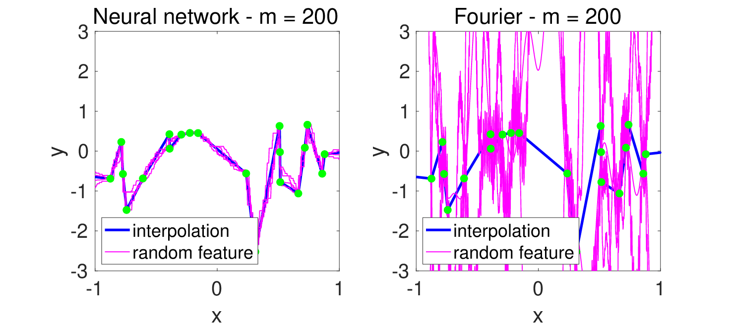
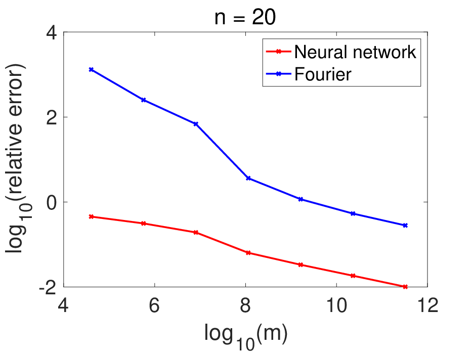
We compare the two random feature expansions, first visually in Figure 1, then numerically in Figure 2, showing that the random feature expansion based on neural networks has better approximation properties.¹¹ 1 Matlab code to reproduce all figures is available at https://www.di.ens.fr/~fbach/neural_splines_online.zip.

Refer to caption — Figure 1: Minimum norm interpolation of the green points by the full RKHS (in blue) and the random feature expansion, for $m=200$ . Left: neural network expansion, right: Fourier expansion. Four different draws of the random features are plotted.

Comparison of leverage scores for $d=1$ .

We want to compare the two random feature expansions, which are of the form

k(x,y)={\mathbb{E}}_{v}[\varphi(x,v)\varphi(y,v)],

for a feature $\varphi(x,v)\in\mathbb{{R}}$ for $v\in\mathcal{V}$ . As described in [12, Section 4], to assess the capacity of random feature expansions to approximate the initial function space, a key quantity is the “leverage score”

v\mapsto\langle\varphi(\cdot,v),(\Sigma+\lambda I)^{-1}\varphi(\cdot,v)\rangle_{L_{2}({\mathbb{B}}^{d}(R))},

where $\Sigma={\mathbb{E}}_{v}\Big[\varphi(\cdot,v)\otimes_{L_{2}({\mathbb{B}}^{d}(R))}\varphi(\cdot,v)\Big]$ is an integral operator on ${L_{2}({\mathbb{B}}^{d}(R))}$ . The maximal leverage score over $v\in\mathcal{V}$ has a direct influence on the number of needed random features to get a $\lambda$ -approximation in $L_{2}$ -norm of the RKHS ball of the original RKHS: from [12, Prop. 1], up to logarithmic terms, the maximal leverage score is proportional to the number $m$ of necessary random features.

In Appendix C, we compute these leverage scores explicitly for $d=1$ , and we see that for the neural network features, the maximal leverage score diverges as $1/\sqrt{\lambda}$ when $\lambda$ tends to zero, while for random Fourier features, they diverge faster as $1/\lambda$ , explaining the empirical superiority seen above.

5.4 A new random feature expansions for all $\alpha$

For all $\alpha$ , we provided a new kernel $k_{d}^{(\alpha)}$ that makes the classical multivariate spline positive-definite, together with a random feature expansion, that can be used for efficient estimation. See [7] for an analysis.

Other kernels lead to RKHS norms that are equivalent to the same Sobolev norm, such as the Matérn kernels [23, page 84]. These have a natural random Fourier feature expansion (with empirically the same behavior as shown for $\alpha=0$ above), while ours are based on neural networks, with a better behavior when used within random feature expansions.

6 Conclusion

In this paper, we provided new random feature expansions for kernels associated with splines, leading to better properties for Sobolev space on the Euclidean balls than existing expansions based on the Fourier transform. As done by [14] with feature expansions based on spherical harmonics, this link could be used to provide explicit approximation bounds for neural networks for a large number of neurons (where input weights are also estimated).

Acknowledgements

We thank Nicolas Le Roux and Alessandro Rudi for the interesting discussions related to this work. We acknowledge support from the French government under the management of the Agence Nationale de la Recherche as part of the “Investissements d’avenir” program, reference ANR-19-P3IA-0001 (PRAIRIE 3IA Institute), as well as from the European Research Council (grant SEQUOIA 724063).

Appendix A A few lemmas about uniform distributions on the sphere

If $w$ is uniform on the unit sphere, then:

$\displaystyle{\mathbb{E}}[\|w^{\top}z\|^{2\alpha+1}]$	$\displaystyle=$	$\displaystyle\\|z\\|_{2}^{2\alpha+1}\frac{\Gamma(1+\alpha)\Gamma(\frac{d}{2})}{\Gamma(\frac{1}{2})\Gamma(\frac{d}{2}+\frac{1}{2}+\alpha)}$
$\displaystyle{\mathbb{E}}[(w^{\top}z)^{2\alpha}]$	$\displaystyle=$	$\displaystyle\\|z\\|_{2}^{2\alpha}\frac{\Gamma(\frac{1}{2}+\alpha)\Gamma(\frac{d}{2})}{\Gamma(\frac{1}{2})\Gamma(\frac{d}{2}+\alpha)}$
$\displaystyle{\mathbb{E}}[(w^{\top}z)^{2}]$	$\displaystyle=$	$\displaystyle\\|z\\|_{2}^{2}/d$
$\displaystyle{\mathbb{E}}[z^{\top}ww^{\top}t]$	$\displaystyle=$	$\displaystyle\frac{1}{d}z^{\top}t$
$\displaystyle{\mathbb{E}}[(z^{\top}ww^{\top}t)^{2}]$	$\displaystyle=$	$\displaystyle\frac{1}{d(d+2)}\big[2(z^{\top}t)^{2}+z^{\top}z\cdot t^{\top}t\big].$

This is obtained from $w_{1}^{2}$ having a Beta distribution with parameters $(\frac{1}{2},\frac{d-1}{2})$ , and using invariance by rotation.

Appendix B Proof for expressions of RKHS norms, $d=1$

B.1 Proof of Proposition 1

We have $\displaystyle\int_{-R}^{R}(x-b)_{+}^{\alpha}(y-b)^{\alpha}_{+}db=\int_{R}^{\min\{x,y\}}(x-b)^{\alpha}(y-b)^{\alpha}db,$ which we can reformulate with $s=\frac{x+y}{2}$ and $\delta=\frac{x-y}{2}$ , leading to $x=s+\delta$ and $y=s-\delta$ , with $\min\{x,y\}=s-|\delta|$ . We get:

$\displaystyle\int_{-R}^{R}(x-b)_{+}^{\alpha}(y-b)^{\alpha}_{+}db$	$\displaystyle=$	$\displaystyle\int_{-R}^{s-\|\delta\|}(s+\delta-b)^{\alpha}(s-\delta-b)^{\alpha}db=\int_{-R}^{s-\|\delta\|}((s-b)^{2}-\delta^{2})^{\alpha}db$
	$\displaystyle=$	$\displaystyle\int_{-R}^{s-\|\delta\|}\sum_{i=0}^{\alpha}{\alpha\choose i}(s-b)^{2i}(-1)^{i-\alpha}\delta^{2\alpha-2i}db$
	$\displaystyle=$	$\displaystyle\sum_{i=0}^{\alpha}{\alpha\choose i}\frac{1}{2i+1}\Big[(R+s)^{2i+1}-\|\delta\|^{2i+1}\Big](-1)^{i-\alpha}\delta^{2\alpha-2i}$
	$\displaystyle=$	$\displaystyle\sum_{i=0}^{\alpha}{\alpha\choose i}\frac{(-1)^{i-\alpha}}{2i+1}(R+s)^{2i+1}\delta^{2\alpha-2i}-\sum_{i=0}^{\alpha}{\alpha\choose i}\frac{(-1)^{i-\alpha}}{2i+1}\times\|\delta\|^{2\alpha+1}$
	$\displaystyle=$	$\displaystyle A_{\alpha}(x,y)-B_{\alpha}\|x-y\|^{2\alpha+1},$

with

$\displaystyle A_{\alpha}$	$\displaystyle=$	$\displaystyle\sum_{i=0}^{\alpha}{\alpha\choose i}\frac{(-1)^{i-\alpha}}{2i+1}(R+s)^{2i+1}\delta^{2\alpha-2i}=\int_{-y}^{R}(x+b)^{\alpha}(y+b)^{\alpha}db$
$\displaystyle B_{\alpha}$	$\displaystyle=$	$\displaystyle\frac{1}{2^{2\alpha+1}}\sum_{i=0}^{\alpha}{\alpha\choose i}\frac{(-1)^{i-\alpha}}{2i+1}=\frac{1}{2^{2\alpha+1}}\int_{0}^{1}\sum_{i=0}^{\alpha}{\alpha\choose i}(-1)^{i-\alpha}x^{2i}dx$
	$\displaystyle=$	$\displaystyle\frac{(-1)^{\alpha}}{2^{2\alpha+1}}\int_{0}^{1}(1-x^{2})^{\alpha}dx=\frac{(-1)^{\alpha}}{2^{2\alpha+2}}2^{2\alpha+1}\int_{0}^{1}u^{\alpha}(1-u)^{\alpha}du=\frac{(-1)^{\alpha}}{2}\frac{\Gamma(\alpha+1)^{2}}{\Gamma(2\alpha+2)},$

using the change of variable $\frac{1+x}{2}=u$ , $\frac{1-x}{2}=1-u$ . This leads to, using symmetries:

$\displaystyle k_{d}^{(\alpha)}(x,y)$	$\displaystyle=$	$\displaystyle\frac{1}{4R}\int_{-y}^{R}(x+b)^{\alpha}(y+b)^{\alpha}db+\frac{1}{4R}\int_{y}^{R}(-x+b)^{\alpha}(-y+b)^{\alpha}db$
		$\displaystyle\hskip 227.62204pt-\frac{(-1)^{\alpha}}{4R}\frac{\Gamma(\alpha+1)^{2}}{\Gamma(2\alpha+2)}\|x-y\|^{2\alpha+1}$
	$\displaystyle=$	$\displaystyle\frac{1}{4R}\int_{-y}^{R}(x+b)^{\alpha}(y+b)^{\alpha}db+\frac{1}{4R}\int_{-R}^{-y}(-x-b)^{\alpha}(-y-b)^{\alpha}db$
		$\displaystyle\hskip 227.62204pt-\frac{(-1)^{\alpha}}{4R}\frac{\Gamma(\alpha+1)^{2}}{\Gamma(2\alpha+2)}\|x-y\|^{2\alpha+1}$
	$\displaystyle=$	$\displaystyle\frac{1}{4R}\int_{-R}^{R}(x+b)^{\alpha}(y+b)^{\alpha}db-\frac{(-1)^{\alpha}}{4R}\frac{\Gamma(\alpha+1)^{2}}{\Gamma(2\alpha+2)}\|x-y\|^{2\alpha+1}.$

We can then expand using the binomial formula.

B.2 Proof of Proposition 2

If we have the representation, for $f$ with $\alpha+1$ continuous derivatives:

\forall x\in[-R,R],f(x)=\frac{1}{4R}\int_{-R}^{R}\big[\eta_{+}(b)(x-b)_{+}^{\alpha}+\eta_{-}(b)(b-x)_{+}^{\alpha}\big]db,

then by taking the $(\alpha+1)$ -derivative, we must have:

f^{(\alpha+1)}(x)=\frac{\alpha!}{4R}\eta_{+}(x)+\frac{\alpha!}{4R}(-1)^{\alpha+1}\eta_{-}(x).

We thus have:

	$\displaystyle\eta_{+}(x)$	$\displaystyle=$	$\displaystyle\frac{2R}{\alpha!}f^{(\alpha+1)}(x)+c(x)$
	$\displaystyle\eta_{-}(x)$	$\displaystyle=$	$\displaystyle(-1)^{\alpha+1}\frac{2R}{\alpha!}f^{(\alpha+1)}(x)+(-1)^{\alpha}c(x)$

for a certain function $c:[-R,R]\to\mathbb{{R}}$ . We have from Taylor formula with integral remainder:

$\displaystyle f(x)$	$\displaystyle\!\!=\!\!$	$\displaystyle\sum_{i=0}^{\alpha}\frac{f^{(i)}(-R)}{i!}(x+R)^{i}+\int_{-R}^{R}\frac{f^{(\alpha+1)}(b)}{\alpha!}(x-b)_{+}^{\alpha}db$
$\displaystyle f(x)$	$\displaystyle\!\!=\!\!$	$\displaystyle\sum_{i=0}^{\alpha}\frac{(-1)^{i}f^{(i)}(R)}{i!}(R-x)^{i}-(-1)^{\alpha}\int_{-R}^{R}\frac{f^{(\alpha+1)}(b)}{\alpha!}(b-x)_{+}^{\alpha}db,\mbox{ and by averaging them},$
$\displaystyle f(x)$	$\displaystyle\!\!=\!\!$	$\displaystyle\frac{1}{2}\sum_{i=0}^{\alpha}\Big[\frac{f^{(i)}(-R)}{i!}(x+R)^{i}+\frac{(-1)^{i}f^{(i)}(R)}{i!}(R-x)^{i}\Big]$
		$\displaystyle\hskip 142.26378pt+\frac{1}{2}\int_{-R}^{R}\frac{f^{(\alpha+1)}(b)}{\alpha!}\big[(x-b)_{+}^{\alpha}-(-1)^{\alpha}(b-x)_{+}^{\alpha}\big]db.$

Given our expression for $\eta_{+}$ and $\eta_{-}$ , this implies that for all $x\in[-R,R]$

	$\displaystyle\frac{1}{2}\sum_{i=0}^{\alpha}\Big[\frac{f^{(i)}(-R)}{i!}(x+R)^{i}+\frac{(-1)^{i}f^{(i)}(R)}{i!}(R-x)^{i}\Big]$	$\displaystyle=$	$\displaystyle\frac{1}{4R}\int_{-R}^{R}\big[c(b)(x-b)_{+}^{\alpha}+(-1)^{\alpha}c(b)(b-x)_{+}^{\alpha}]db$
		$\displaystyle=$	$\displaystyle\frac{1}{4R}\int_{-R}^{R}c(b)(x-b)^{\alpha}db,$

leading to constraints on $\displaystyle\int_{-R}^{R}c(b)b^{i}$ for $i\in\{0,\dots,\alpha\}$ . The optimal $c$ is obtained by minimizing:

\frac{1}{4R}\int_{-R}^{R}\big[\eta_{+}(b)^{2}+\eta_{-}(b)^{2}\big]db=\frac{2R}{\alpha!^{2}}\int_{-R}^{R}f^{(\alpha+1)}(b)^{2}db+\frac{1}{2R}\int_{-R}^{R}c(b)^{2}db.

Thus $c$ has to be a polynomial of degree less than $\alpha$ , with coefficients which are linear combinations of $f^{(i)}(\pm R)$ for $i\in\{0,\dots,\alpha\}$ . This leads to the desired result.

B.3 Polynomial kernel in one dimension

Given a polynomial $P$ on $\mathbb{{R}}$ of degree less than $\alpha$ (or equal), if we can write it as:

P(x)=\frac{1}{2R}\int_{-R}^{R}\eta(b)(x-b)^{\alpha}db,

(6)

then its squared RKHS norm (for $k_{1}^{(\alpha),({\rm pol})})$ is equal to the infimum of $\displaystyle\frac{1}{4R}\int_{-R}^{R}\eta(b)^{2}db$ . Given the representation in Eq. (6), we have:

P^{(k)}(0)=\frac{1}{2R}\frac{\alpha!}{(\alpha-k)!}\int_{-R}^{R}\eta(b)(-b)^{\alpha-k}db=\frac{(-1)^{\alpha-k}}{2R}\frac{\alpha!}{(\alpha-k)!}\int_{-R}^{R}\eta(b)b^{\alpha-k}db,

which is equal to $\displaystyle\frac{(-1)^{\alpha-k}}{2R}\frac{\alpha!}{(\alpha-k)!}\langle\eta,Q_{\alpha-k}\rangle_{L_{2}({\mathbb{B}}^{d}(R))}$ , where $Q_{j}(b)=b^{j}$ . Thus, given that we want to minimize $\langle\eta,\eta\rangle_{L_{2}({\mathbb{B}}^{d}(R))}$ , the solution has to be a polynomial $\eta=\sum_{j=0}^{\alpha}s_{j}Q_{j}$ , with $s\in\mathbb{{R}}^{\alpha+1}$ minimizing

\sum_{i,j=0}^{\alpha}s_{i}s_{j}\langle Q_{i},Q_{j}\rangle_{L_{2}({\mathbb{B}}^{d}(R))}

such that $\displaystyle(-1)^{j}2R\frac{j!}{\alpha!}P^{(\alpha-j)}(0)=\sum_{i=0}^{\alpha}s_{i}\langle Q_{i},Q_{j}\rangle_{L_{2}({\mathbb{B}}^{d}(R))}$ for all $j\in\{0,\dots,\alpha\}$ . If $P=\sum_{j=0}^{\alpha}t_{j}Q_{j}$ , we obtain $\displaystyle(-1)^{j}2R{\alpha\choose j}^{-1}t_{\alpha-j}=\sum_{i=0}^{\alpha}s_{i}\langle Q_{i},Q_{j}\rangle_{L_{2}({\mathbb{B}}^{d}(R))}$ . Since the Gram matrix of the monomials is invertible, the optimal $s$ is a linear function of the coefficients $t$ . Thus the norm of $P$ is a positive-definite quadratic form in the coefficients. Hence the norm is equivalent to the $L_{2}$ -norm on the space of polynomials of degree less than $\alpha$ (or equal).

B.4 Polynomial kernel in dimension $d\geqslant 1$

We can apply the same reasoning as in the section above and need to show that we can represent all polynomials of degree less than $\alpha$ as

P(x)=\frac{1}{2R}\int_{-R}^{R}\int_{{\mathbb{S}}^{d}}\eta(w,b)(w^{\top}x+b)^{\alpha}dwdb,

for $\eta(w,b)$ square integrable. By taking all partial derivatives at $x=0$ , this imposes that all

\int_{-R}^{R}\int_{{\mathbb{S}}^{d}}\eta(w,b)w_{1}^{u_{1}}\cdots w_{d}^{u_{d}}b^{v}dwdb

are fixed, for $u_{1}+\dots+u_{d}+v=\alpha$ , and since the family of polynomials $(w,b)\mapsto w_{1}^{u_{1}}\cdots w_{d}^{u_{d}}b^{v}$ is linearly independent in $L_{2}({\mathbb{S}}^{d}\times[-1,1])$ , the same reasoning above leads to an RKHS norm which is equivalent the $L_{2}$ -norm on the space of polynomials of degree less than $\alpha$ (or equal).

Appendix C Computing leverage scores

In this section, we explicitly compute leverage scores for $d=1$ and $\alpha=0$ for the two expansions.

C.1 General solution

We consider $d=1$ , $R=1$ , and the classical integral operator for the uniform distribution on $[-1,1]$ :

\Sigma f(x)=\frac{1}{2}\int_{-1}^{1}k_{1}^{(0)}(x,y)f(y)dy=\frac{1}{4}\int_{-1}^{1}f(y)dy-\frac{1}{8}\int_{-1}^{1}|x-y|f(y)dy.

Given a function $g\in L_{2}([-1,1])$ , we aim to compute the leverage score:

\frac{1}{2}\int_{-1}^{1}g(x)\big[(\Sigma+\lambda I)^{-1}g\big](x)dx.

We thus compute $f=(\Sigma+\lambda I)^{-1}g$ , which is such that:

g(x)=\frac{1}{4}\int_{-1}^{1}f(y)dy-\frac{1}{8}\int_{-1}^{1}|x-y|f(x)dy+\lambda f(x).

By taking two derivatives and using the fact that the second-order derivative of $x\mapsto|x-y|$ is $2\delta_{y}$ , we get:

g^{\prime\prime}(x)=\lambda f^{\prime\prime}(x)-\frac{1}{4}f(x).

Once we know a solution $f_{0}$ for the ordinary differential equation above, then all solutions are obtained as

f(x)=f_{0}(x)+A\cosh\frac{x}{2\sqrt{\lambda}}+B\sinh\frac{x}{2\sqrt{\lambda}},

(7)

for some $A,B\in\mathbb{{R}}$ .

Obtaining a solution in “closed-form”.

We can solve the ODE in $f$ using standard techniques [24], by writing $f(x)=e^{\frac{x}{2\sqrt{\lambda}}}a(x)$ , so that

	$\displaystyle g^{\prime\prime}(x)$	$\displaystyle=$	$\displaystyle\lambda e^{\frac{x}{2\sqrt{\lambda}}}a^{\prime\prime}(x)+{\sqrt{\lambda}}e^{\frac{x}{2\sqrt{\lambda}}}a^{\prime}(x)$
	$\displaystyle e^{-\frac{x}{2\sqrt{\lambda}}}g^{\prime\prime}(x)$	$\displaystyle=$	$\displaystyle\lambda a^{\prime\prime}(x)+{\sqrt{\lambda}}a^{\prime}(x).$

We then write $a^{\prime}(x)=e^{-\frac{x}{\sqrt{\lambda}}}c(x)$ , so that

e^{-\frac{x}{2\sqrt{\lambda}}}g^{\prime\prime}(x)=\lambda e^{-\frac{x}{\sqrt{\lambda}}}c^{\prime}(x),

and thus

c^{\prime}(x)=\frac{1}{\lambda}e^{\frac{x}{2\sqrt{\lambda}}}g^{\prime\prime}(x),

leading to a particular solution by integration:

c(x)=\frac{1}{2\lambda}\int_{-1}^{1}e^{\frac{y}{2\sqrt{\lambda}}}g^{\prime\prime}(y)\mathop{\rm sign}(x-y)dy.

Moreover, we get a particular solution:

$\displaystyle a(x)$	$\displaystyle=$	$\displaystyle\frac{1}{2}\int_{-1}^{1}e^{-\frac{y}{\sqrt{\lambda}}}c(y)\mathop{\rm sign}(x-y)dy$
	$\displaystyle=$	$\displaystyle\frac{1}{4\lambda}\int_{-1}^{1}e^{-\frac{y}{\sqrt{\lambda}}}\int_{-1}^{1}e^{\frac{t}{2\sqrt{\lambda}}}g^{\prime\prime}(t)\mathop{\rm sign}(y-t)dt\mathop{\rm sign}(x-y)dy$
$\displaystyle f(x)$	$\displaystyle=$	$\displaystyle\frac{1}{4\lambda}\int_{-1}^{1}\int_{-1}^{1}e^{\frac{x}{2\sqrt{\lambda}}}e^{-\frac{y}{\sqrt{\lambda}}}e^{\frac{t}{2\sqrt{\lambda}}}g^{\prime\prime}(t)\mathop{\rm sign}(y-t)\mathop{\rm sign}(x-y)dydt,$

with all solutions obtained by adding $A\cosh\frac{x}{2\sqrt{\lambda}}+B\sinh\frac{x}{2\sqrt{\lambda}}$ .

Finding constants $A$ and $B$ .

We have for the unique solution $f$ of $g=(\Sigma+\lambda I)f$ :

$\displaystyle g(1)$	$\displaystyle=$	$\displaystyle\frac{1}{4}\int_{-1}^{1}f(y)dy-\frac{1}{8}\int_{-1}^{1}(1-y)f(y)dy+\lambda f(1)$
$\displaystyle g(-1)$	$\displaystyle=$	$\displaystyle\frac{1}{4}\int_{-1}^{1}f(y)dy-\frac{1}{8}\int_{-1}^{1}(1+y)f(y)dy+\lambda f(-1),\mbox{ leading to}$
$\displaystyle g(1)+g(-1)$	$\displaystyle=$	$\displaystyle\frac{1}{4}\int_{-1}^{1}f(y)dy+\lambda[f(1)+f(-1)]$	(8)
$\displaystyle g(1)-g(-1)$	$\displaystyle=$	$\displaystyle\frac{1}{4}\int_{-1}^{1}yf(y)dy+\lambda[f(1)-f(-1)].$	(9)

For $f(x)=\cosh\frac{x}{2\sqrt{\lambda}}$ , we have: $\displaystyle\int_{-1}^{1}f(x)dx=4\sqrt{\lambda}\sinh\frac{1}{2\sqrt{\lambda}}.$

For $f(x)=\sinh\frac{x}{2\sqrt{\lambda}}$ , we have: $\displaystyle\int_{-1}^{1}xf(x)dx=4\sqrt{\lambda}\cosh\frac{1}{2\sqrt{\lambda}}-8\lambda\sinh\frac{1}{2\sqrt{\lambda}}.$

Thus, for our solution in Eq. (7):

	$\displaystyle g(1)+g(-1)$	$\displaystyle=$	$\displaystyle\frac{1}{4}\int_{-1}^{1}f_{0}(y)dy+\lambda[f_{0}(1)+f_{0}(-1)]+A\Big[\sqrt{\lambda}\sinh\frac{1}{2\sqrt{\lambda}}+2\lambda\cosh\frac{1}{2\sqrt{\lambda}}\Big]$
	$\displaystyle g(1)-g(-1)$	$\displaystyle=$	$\displaystyle\frac{1}{4}\int_{-1}^{1}yf_{0}(y)dy+\lambda[f_{0}(1)-f_{0}(-1)]+B\sqrt{\lambda}\cosh\frac{1}{2\sqrt{\lambda}}.$

Therefore, to obtain $A$ and $B$ , we simply need to compute $f_{0}(1)$ , $f_{0}(-1)$ as well as $\displaystyle\int_{-1}^{1}f_{0}(y)dy$ and $\displaystyle\int_{-1}^{1}yf_{0}(y)dy$ .

C.2 Neural networks

We consider $g(x)=1_{x>b}=(x-b)_{+}^{0}$ , we then consider $f_{0}(x)=1_{x>b}\frac{1}{\lambda}\cosh\frac{x-b}{2\sqrt{\lambda}}$ . We have:

$\displaystyle g(x)-\lambda f_{0}(x)$	$\displaystyle=$	$\displaystyle 1_{x>b}\big[1-\cosh\frac{x-b}{2\sqrt{\lambda}}\big]$
$\displaystyle g^{\prime}(x)-\lambda f_{0}^{\prime}(x)$	$\displaystyle=$	$\displaystyle-\frac{1}{2\sqrt{\lambda}}1_{x>b}\sinh\frac{x-b}{2\sqrt{\lambda}}$
$\displaystyle g^{\prime\prime}(x)-\lambda f_{0}^{\prime\prime}(x)$	$\displaystyle=$	$\displaystyle-\frac{1}{4\lambda}1_{x>b}\cosh\frac{x-b}{2\sqrt{\lambda}}=-\frac{1}{4}f_{0}(x),$

and thus $f_{0}$ is a particular solution. We have:

$\displaystyle f_{0}(1)+f_{0}(-1)$	$\displaystyle=$	$\displaystyle f_{0}(1)-f_{0}(-1)=f_{0}(1)=\frac{1}{\lambda}\cosh\frac{1-b}{2\sqrt{\lambda}}$
$\displaystyle\int_{-1}^{1}f_{0}(x)dx$	$\displaystyle=$	$\displaystyle\int_{b}^{1}\frac{1}{\lambda}\cosh\frac{x-b}{2\sqrt{\lambda}}dx=\frac{2}{\sqrt{\lambda}}\sinh\frac{1-b}{2\sqrt{\lambda}}$
$\displaystyle\int_{-1}^{1}xf_{0}(x)dx$	$\displaystyle=$	$\displaystyle\int_{b}^{1}\frac{1}{\lambda}x\cosh\frac{x-b}{2\sqrt{\lambda}}dx=\int_{b}^{1}\frac{1}{\lambda}b\cosh\frac{x-b}{2\sqrt{\lambda}}dx+\int_{b}^{1}\frac{1}{\lambda}(x-b)\cosh\frac{x-b}{2\sqrt{\lambda}}dx$
	$\displaystyle=$	$\displaystyle\frac{2b}{\sqrt{\lambda}}\sinh\frac{1-b}{2\sqrt{\lambda}}+\frac{2}{\sqrt{\lambda}}\Big[(1-b)\sinh\frac{1-b}{2\sqrt{\lambda}}-2\sqrt{\lambda}\cosh\frac{1-b}{2\sqrt{\lambda}}\Big]$
	$\displaystyle=$	$\displaystyle\frac{2}{\sqrt{\lambda}}\Big[\sinh\frac{1-b}{2\sqrt{\lambda}}-2\sqrt{\lambda}\cosh\frac{1-b}{2\sqrt{\lambda}}\Big].$

Thus

	$\displaystyle\frac{1}{2}$	$\displaystyle=$	$\displaystyle\frac{1}{2\sqrt{\lambda}}\sinh\frac{1-b}{2\sqrt{\lambda}}+\cosh\frac{1-b}{2\sqrt{\lambda}}+2\lambda A\Big[\frac{1}{2\sqrt{\lambda}}\sinh\frac{1}{2\sqrt{\lambda}}+\cosh\frac{1}{2\sqrt{\lambda}}\Big]$
	$\displaystyle\frac{1}{2}$	$\displaystyle=$	$\displaystyle\frac{1}{2\sqrt{\lambda}}\sinh\frac{1-b}{2\sqrt{\lambda}}+B\sqrt{\lambda}\cosh\frac{1}{2\sqrt{\lambda}},$

which allows to solve for $A$ and $B$ . Moreover

$\displaystyle\int_{-1}^{1}f(x)g(x)dx$	$\displaystyle=$	$\displaystyle\int_{-1}^{1}g(x)\big[f_{0}(x)+A\cosh\frac{x}{2\sqrt{\lambda}}+B\sinh\frac{x}{2\sqrt{\lambda}}\big]dx$
	$\displaystyle=$	$\displaystyle\frac{2}{\sqrt{\lambda}}\sinh\frac{1-b}{2\sqrt{\lambda}}+2A\sqrt{\lambda}\big[\sinh\frac{1}{2\sqrt{\lambda}}-\sinh\frac{b}{2\sqrt{\lambda}}\big]+2B\sqrt{\lambda}\big[\cosh\frac{1}{2\sqrt{\lambda}}-\cosh\frac{b}{2\sqrt{\lambda}}\big]$
	$\displaystyle=$	$\displaystyle\frac{2}{\sqrt{\lambda}}\sinh\frac{1-b}{2\sqrt{\lambda}}+\frac{1}{\sqrt{\lambda}}\frac{\big[\frac{1}{2}-\frac{1}{2\sqrt{\lambda}}\sinh\frac{1-b}{2\sqrt{\lambda}}-\cosh\frac{1-b}{2\sqrt{\lambda}}\big]}{\frac{1}{2\sqrt{\lambda}}\sinh\frac{1}{2\sqrt{\lambda}}+\cosh\frac{1}{2\sqrt{\lambda}}}\big[\sinh\frac{1}{2\sqrt{\lambda}}-\sinh\frac{b}{2\sqrt{\lambda}}\big]$
		$\displaystyle+\frac{1-\frac{1}{\sqrt{\lambda}}\sinh\frac{1-b}{2\sqrt{\lambda}}}{\cosh\frac{1}{2\sqrt{\lambda}}}\big[\cosh\frac{1}{2\sqrt{\lambda}}-\cosh\frac{b}{2\sqrt{\lambda}}\big],$

which is our desired quantity (multiplied by 2). This quantity is maximized at $b=0$ , for which we have the value:

			$\displaystyle\frac{2}{\sqrt{\lambda}}\sinh\frac{1}{2\sqrt{\lambda}}+\frac{1}{\sqrt{\lambda}}\frac{\big[\frac{1}{2}-\frac{1}{2\sqrt{\lambda}}\sinh\frac{1}{2\sqrt{\lambda}}-\cosh\frac{1}{2\sqrt{\lambda}}\big]}{\frac{1}{2\sqrt{\lambda}}\sinh\frac{1}{2\sqrt{\lambda}}+\cosh\frac{1}{2\sqrt{\lambda}}}\big[\sinh\frac{1}{2\sqrt{\lambda}}\big]+\frac{1-\frac{1}{\sqrt{\lambda}}\sinh\frac{1}{2\sqrt{\lambda}}}{\cosh\frac{1}{2\sqrt{\lambda}}}\big[\cosh\frac{1}{2\sqrt{\lambda}}-1\big]$
		$\displaystyle=$	$\displaystyle\frac{1}{\sqrt{\lambda}}\frac{\big[\frac{1}{2}+\frac{1}{2\sqrt{\lambda}}\sinh\frac{1}{2\sqrt{\lambda}}-\cosh\frac{1}{2\sqrt{\lambda}}\big]}{\frac{1}{2\sqrt{\lambda}}\sinh\frac{1}{2\sqrt{\lambda}}+\cosh\frac{1}{2\sqrt{\lambda}}}\big[\sinh\frac{1}{2\sqrt{\lambda}}\big]+\big[{1-\frac{1}{\sqrt{\lambda}}\sinh\frac{1}{2\sqrt{\lambda}}}\big]\cdot\big[1-\frac{1}{\cosh\frac{1}{2\sqrt{\lambda}}}\big]$
		$\displaystyle=$	$\displaystyle\Big[1+\frac{1/2}{\frac{1}{2\sqrt{\lambda}}\sinh\frac{1}{2\sqrt{\lambda}}+\cosh\frac{1}{2\sqrt{\lambda}}}\Big]\frac{1}{\sqrt{\lambda}}\sinh\frac{1}{2\sqrt{\lambda}}+\big[{1-\frac{1}{\sqrt{\lambda}}\sinh\frac{1}{2\sqrt{\lambda}}}\big]\cdot\big[1-\frac{1}{\cosh\frac{1}{2\sqrt{\lambda}}}\big]$
		$\displaystyle=$	$\displaystyle\frac{\frac{1}{2\sqrt{\lambda}}\sinh\frac{1}{2\sqrt{\lambda}}}{\frac{1}{2\sqrt{\lambda}}\sinh\frac{1}{2\sqrt{\lambda}}+\cosh\frac{1}{2\sqrt{\lambda}}}+\big[1-\frac{1}{\cosh\frac{1}{2\sqrt{\lambda}}}\big]+\frac{1}{\sqrt{\lambda}}\frac{\sinh\frac{1}{2\sqrt{\lambda}}}{\cosh\frac{1}{2\sqrt{\lambda}}}.$

The maximal leverage score has thus order $\frac{1}{2\sqrt{\lambda}}$ .

C.3 Fourier feature

We consider $g(x)=e^{i\omega x}$ so that we can obtain both $\cos\omega x$ and $\sin\omega x$ . Then we can take $f_{0}(x)=\frac{\omega^{2}}{\lambda\omega^{2}+\frac{1}{4}}e^{i\omega x}$ as a special solution, since

\lambda f_{0}^{\prime\prime}(x)-\frac{1}{4}f_{0}(x)=\omega^{2}\frac{-\lambda\omega^{2}-\frac{1}{4}}{\lambda\omega^{2}+\frac{1}{4}}e^{i\omega x}=g^{\prime\prime}(x).

We get, from Eq. (8) and Eq. (9):

	$\displaystyle 2\cos\omega$	$\displaystyle=$	$\displaystyle\frac{\omega^{2}}{4\lambda\omega^{2}+1}\frac{1}{i\omega}2i\sin\omega+\frac{\lambda\omega^{2}}{\lambda\omega^{2}+\frac{1}{4}}2\cos\omega+A\Big[\sqrt{\lambda}\sinh\frac{1}{2\sqrt{\lambda}}+2\lambda\cosh\frac{1}{2\sqrt{\lambda}}\Big]$
	$\displaystyle 2i\sin\omega$	$\displaystyle=$	$\displaystyle\frac{\omega^{2}}{4\lambda\omega^{2}+1}\Big[\frac{1}{\omega^{2}}e^{i\omega x}(1-i\omega x)\Big]_{-1}^{1}+\frac{\lambda\omega^{2}}{\lambda\omega^{2}+\frac{1}{4}}2i\sin\omega+B\sqrt{\lambda}\cosh\frac{1}{2\sqrt{\lambda}}.$

This leads to explicit formulas for the constants $A$ and $B$ :

$\displaystyle\frac{2\cos\omega-2\omega\sin\omega}{4\lambda\omega^{2}+1}$	$\displaystyle=$	$\displaystyle A\Big[\sqrt{\lambda}\sinh\frac{1}{2\sqrt{\lambda}}+2\lambda\cosh\frac{1}{2\sqrt{\lambda}}\Big]$
$\displaystyle\frac{2i\sin\omega}{4\lambda\omega^{2}+1}$	$\displaystyle=$	$\displaystyle\frac{1}{4\lambda\omega^{2}+1}\Big[2i\sin\omega-2i\omega\cos\omega\Big]+B\sqrt{\lambda}\cosh\frac{1}{2\sqrt{\lambda}},\mbox{ leading to}$
$\displaystyle\frac{2i\omega\cos\omega}{4\lambda\omega^{2}+1}$	$\displaystyle=$	$\displaystyle B\sqrt{\lambda}\cosh\frac{1}{2\sqrt{\lambda}}.$

We then get

	$\displaystyle A$	$\displaystyle=$	$\displaystyle\frac{2\cos\omega-2\omega\sin\omega}{4\lambda\omega^{2}+1}\frac{1}{\sqrt{\lambda}\sinh\frac{1}{2\sqrt{\lambda}}+2\lambda\cosh\frac{1}{2\sqrt{\lambda}}}$
	$\displaystyle\frac{B}{i}$	$\displaystyle=$	$\displaystyle\frac{2\omega\cos\omega}{4\lambda\omega^{2}+1}\frac{1}{\sqrt{\lambda}\cosh\frac{1}{2\sqrt{\lambda}}}.$

Thus, the solution for $g(x)=\cos\omega x$ is $\displaystyle f(x)=\frac{\omega^{2}}{\lambda\omega^{2}+\frac{1}{4}}\cos\omega x+A\cosh\frac{x}{2\sqrt{\lambda}}$ , while the solution for $g(x)=\sin\omega x$ is $\displaystyle f(x)=\frac{\omega^{2}}{\lambda\omega^{2}+\frac{1}{4}}\sin\omega x+\frac{B}{i}\sinh\frac{x}{2\sqrt{\lambda}}$ .

Thus, we can compute for $g(x)=\cos\omega x$

$\displaystyle\int_{-1}^{1}f(x)g(x)dx$	$\displaystyle=$	$\displaystyle\int_{-1}^{1}\cos\omega x\Big[\frac{\omega^{2}}{\lambda\omega^{2}+\frac{1}{4}}\cos\omega x+A\cosh\frac{x}{2\sqrt{\lambda}}\Big]dx$
	$\displaystyle=$	$\displaystyle\frac{\omega^{2}}{\lambda\omega^{2}+\frac{1}{4}}\Big(1+\frac{1}{2}\frac{\sin\omega}{\omega}\Big)+A\int_{-1}^{1}\cos\omega x\cosh\frac{x}{2\sqrt{\lambda}}dx$
	$\displaystyle=$	$\displaystyle\frac{\omega^{2}}{\lambda\omega^{2}+\frac{1}{4}}\Big(1+\frac{1}{2}\frac{\sin\omega}{\omega}\Big)+\frac{2A}{\omega^{2}+\frac{1}{4\lambda}}\Big[\frac{1}{2\sqrt{\lambda}}\cos\omega\sinh\frac{1}{2\sqrt{\lambda}}+\omega\sin\omega\cosh\frac{1}{2\sqrt{\lambda}}\Big].$

For $g(x)=\sin\omega x$ , we get:

$\displaystyle\int_{-1}^{1}f(x)g(x)dx$	$\displaystyle=$	$\displaystyle\int_{-1}^{1}\sin\omega x\Big[\frac{\omega^{2}}{\lambda\omega^{2}+\frac{1}{4}}\sin\omega x+\frac{B}{i}\sinh\frac{x}{2\sqrt{\lambda}}\Big]dx$
	$\displaystyle=$	$\displaystyle\frac{\omega^{2}}{\lambda\omega^{2}+\frac{1}{4}}\Big(1-\frac{1}{2}\frac{\sin\omega}{\omega}\Big)+\frac{B}{i}\int_{-1}^{1}\sin\omega x\sinh\frac{x}{2\sqrt{\lambda}}dx$
	$\displaystyle=$	$\displaystyle\frac{\omega^{2}}{\lambda\omega^{2}+\frac{1}{4}}\Big(1-\frac{1}{2}\frac{\sin\omega}{\omega}\Big)+\frac{2B/i}{\omega^{2}+\frac{1}{4\lambda}}\Big[\frac{1}{2\sqrt{\lambda}}\sin\omega\cosh\frac{1}{2\sqrt{\lambda}}-\omega\cos\omega\sinh\frac{1}{2\sqrt{\lambda}}\Big].$

We thus obtain the two leverage scores (divided by 2). We notice that the two leverage scores tend to $1/(2\lambda)$ for $\omega$ tending to infinity, which is the largest value for all $\omega$ .

C.4 Empirical comparisons

As detailed in [25, Appendix A], we can estimate the leverage scores from a grid in $[-1,1]$ with $n$ points by computing $\sum_{i,j=1}^{n}\varphi(x_{i},v)\varphi(x_{j},v)\big[(K+n\lambda I)^{-1}\big]_{ij}$ , and compare with the theoretical expression found above, which match. See Figure 3.

References

[1] Trevor Hastie, Robert Tibshirani, and Jerome H. Friedman. The Elements of Statistical Learning: Data Mining, Inference, and Prediction. Springer, 2009.
[2] Larry Wasserman. All of Nonparametric Statistics. Springer Science & Business Media, 2006.
[3] László Györfi, Michael Kohler, Adam Krzyzak, and Harro Walk. A Distribution-free Theory of Nonparametric Regression. Springer, 2002.
[4] Radford M. Neal. Bayesian Learning for Neural Networks. PhD thesis, University of Toronto, 1995.
[5] Ali Rahimi and Benjamin Recht. Random features for large-scale kernel machines. In Advances in Neural Information Processing Systems, pages 1177–1184, 2008.
[6] Bernhard Schölkopf and Alexander J. Smola. Learning with Kernels: Support Vector Machines, Regularization, Optimization, and Beyond. MIT Press, 2002.
[7] Alessandro Rudi and Lorenzo Rosasco. Generalization properties of learning with random features. In Advances in Neural Information Processing Systems, pages 3215–3225, 2017.
[8] Nicolas Le Roux and Yoshua Bengio. Continuous neural networks. In Artificial Intelligence and Statistics, pages 404–411, 2007.
[9] Jean Duchon. Splines minimizing rotation-invariant semi-norms in Sobolev spaces. In Constructive Theory of Functions of Several Variables, pages 85–100. Springer, 1977.
[10] Martin D. Buhmann. Radial Basis Functions: Theory and Implementations, volume 12. Cambridge University Press, 2003.
[11] Vinod Nair and Geoffrey E. Hinton. Rectified linear units improve restricted Boltzmann machines. In International Conference on Machine Learning, 2010.
[12] Francis Bach. On the equivalence between kernel quadrature rules and random feature expansions. Journal of Machine Learning Research, 18(1):714–751, 2017.
[13] Youngmin Cho and Lawrence K. Saul. Kernel methods for deep learning. In Advances in Neural Information Processing Systems, 2009.
[14] Francis Bach. Breaking the curse of dimensionality with convex neural networks. Journal of Machine Learning Research, 18(1):629–681, 2017.
[15] Meyer Scetbon and Zaid Harchaoui. A spectral analysis of dot-product kernels. In International Conference on Artificial Intelligence and Statistics, pages 3394–3402, 2021.
[16] Amit Daniely, Roy Frostig, and Yoram Singer. Toward deeper understanding of neural networks: The power of initialization and a dual view on expressivity. Advances in Neural Information Processing Systems, 29, 2016.
[17] Agustinus Kristiadi, Matthias Hein, and Philipp Hennig. An infinite-feature extension for Bayesian ReLU nets that fixes their asymptotic overconfidence. Advances in Neural Information Processing Systems, 34, 2021.
[18] Alain Berlinet and Christine Thomas-Agnan. Reproducing Kernel Hilbert Spaces in Probability and Statistics. Springer Science & Business Media, 2011.
[19] Robert A. Adams and John J. F. Fournier. Sobolev Spaces. Academic Press, 2003.
[20] Holger Wendland. Scattered Data Approximation. Cambridge University Press, 2004.
[21] Grace Wahba. Spline Models for Observational Data. SIAM, 1990.
[22] Friedrich Gerard Friedlander, Mark Suresh Joshi, M. Joshi, and Mohan C. Joshi. Introduction to the Theory of Distributions. Cambridge University Press, 1998.
[23] Christopher K. I. Williams and Carl Edward Rasmussen. Gaussian Processes for Machine Learning. MIT Press, 2006.
[24] Carl M. Bender, Steven Orszag, and Steven A. Orszag. Advanced Mathematical Methods for Scientists and Engineers I: Asymptotic Methods and Perturbation Theory, volume 1. Springer Science & Business Media, 1999.
[25] Edouard Pauwels, Francis Bach, and Jean-Philippe Vert. Relating leverage scores and density using regularized Christoffel functions. Advances in Neural Information Processing Systems, 31, 2018.

On the relationship between multivariate splines and infinitely-wide neural networks