![[Uncaptioned image]](2302.03417v1/Logo.jpg)
Institut für Chemie
Masterstudiengang Chemie
Masterarbeit
Ab Initio Magnetic Properties of Rare-Earth Lean Nd-based Hard Magnets
vorgelegt von: Stephan Erdmann
Matrikelnummer: 4546697
Betreuender Gutachter: Herr Prof. Dr. Thorsten Klüner
Zweitgutachter: Herr Dr.-Ing. Halil İbrahim Sözen
Oldenburg, 20.12.2022
Bibliography
List of Abbreviations
Erklärung
Acknowledgements/Danksagung
After writing this work i want to thank Prof. Dr. Thorsten Klüner who enabled me to write this thesis in his working group and for supervising this work. I also want to thank Dr. Ing. Halil İbrahim Sözen for taking the position as the second supervisor. I also want to thank him for helping me with the program package VASP, his tutelage with the different calculations and his general support in this work. Furthermore, I want to thank my friends and especially my family for the support I got in the last years of my studies. Special thanks also go to the working group Theoretische Chemie of the Carl-von-Ossietzky university in Oldenburg who were all ready to help if it was needed. Lastly, I want to thank the team of the HPC-Cluster CARL of the university on which the calculations in this work were done.
Mein besonderer Dank gilt Herrn Prof. Dr. Thorsten Klüner dafür, dass ich diese Abschlussarbeit in seinem Arbeitskreis anfertigen konnte. Weiterhin möchte ich besonders Dr. Ing. Halil İbrahim Sözen für seine Hilfe im Umgang mit dem Programmpaket VASP, seiner Unterstützung bei den Berechnungen, der generellen Betreuung durch ihn sowie der Kontrolle als Zweitprüfer in dieser Arbeit. Ebenfalls danke ich meinen Freunden und besonders meiner Familie welche mich während des Studiums stets unterstützt und mir geholfen haben.
Auch möchte ich generell der Arbeitsgruppe der Theoretischen Chemie in Oldenburg für die Bereitschaft zur Hilfe bei Fragen und für die gute Aufnahme im Arbeitskreis danken. Zuletzt möchte ich mich beim Team des HPC-Clusters CARL der Universität Oldenburg bedanken, auf dem die Berechnungen in dieser Arbeit durchgeführt wurden.
Chapter 1 Introduction to Permanent Magnets and Magnetism
Magnetic materials have played a critical role in the development of electric motors and renewable energy technologies in the last years and are an essential part of many other applications like generators or actuators. Since the need and demand for these technologies are steadily increasing, more and more effort is put into the development of these materials [1]. A big share of this interest is focused on the improvement of rare-earth-based hard magnetic materials that are mostly composed of rare-earth (RE) and transition metal (TM) elements. Due to resource criticality, a big focus is devoted to the reduction of the rare-earth elements in these compounds and on the development of new rare-earth lean or rare-earth free hard magnets [2, 3].
In the first chapter some fundamental and basic magnetic properties such as magnetic moment , magnetization , the maximum energy product , the Curie temperature and the magnetocrystalline anisotropy energy (MAE) are explained to provide a robust understanding for the readers, who are unfamiliar with the topic. In the second part, the historical development of magnetic materials is reported to demonstrate the historical impact of magnets on world development. In the third part, the situation of the current global market and the main usage fields of hard magnetic materials in the last decade are described. At the end of this chapter, the motivation for this thesis is explained.
1.1 Basic Properties of Magnets and Fundamentals
Since the discovery of the first magnetic material, which were naturally magnetized pieces of iron called lodestone, its properties to attract ferrous materials has drawn the attention of many scientists and researchers to it. These properties had a great impact on the development of the world. For instance, the invention of the compass, one of the earliest magnetic devices, made the navigation on sea much easier and also enabled much larger explorations. These explorations included the discovery of America by Christopher Columbus in 1492 or the voyage around the world by Ferdinand Magellan from 1519 to 1522 [4].
The origin of magnetism can be attributed to the magnetic moments of the different atoms in a compound. The classical Bohr definition explains their origin in the motion of an electrical charge, in other words of electrons, and the resulting magnetic field that is generated with their orbital motion. This orbital motion generates an orbital magnetic moment and a spin magnetic moment associated with it, both of which are measured in Bohr magneton [4, 5, 6]. The intrinsic spin angular momentum of electrons is according to the quantum mechanical definition . The total magnetic moment is therefore made out of the orbital (L) and the spin (S) magnetic moment that has two ways to be put together in the forms of LS and JJ couplings with J = L+S. When the electron shell of an element is filled completely the electrons pair themselves with those electrons that have an opposing intrinsic magnetic moment. This leads to an overall total magnetic moment of zero.
Until the 19 century, the shape of magnets was strongly restricted due to the shape-dependent demagnetization caused by the internal magnetic field that occurred in these materials ( = - NM, with N as the shape-dependent demagnetization factor and M as the magnetization). This limited the shape of magnets to be bar and needle-like. A small improvement was the development of magnets in the shape of a horseshoe that avoided the self-demagnetization problem but still restricted the shape to a U-form. Nevertheless, these magnets at least led in combination with copper coils and iron to the first magnetic motors and generators in the 19 century [4, 6].
When the first ferrimagnetic hexagonal ferrites were discovered in 1951, a better understanding of the coercivity led to further progress and enabled the manufacturing of magnets with a coercivity higher than their spontaneous magnetization and a break of the shape restrictions. At that time, it was possible to design magnets in every way possible, which caused a significant increase in usability. Ideally, a high coercivity and a high magnetization are desired for hard magnetic materials. This can best be explained with the hysteresis loop (Fig. 1.1), a plot of the magnetization against the magnetic field strength [4, 5, 6].

In the hysteresis loop, the magnetization starts at zero at point 1 and increases with the magnetic field strength until the maximum at point 2 is reached. This maximum is the magnetization saturation and describes the maximum possible magnetization for a compound. In this process, the magnetic domains in the material, small regions with the same direction of the magnetic moments, are at first oriented in different directions to minimize the magnetostatic energy. When the material reaches , all the domain walls move in the direction of the external field and align parallel to this direction. Once the magnetic field is reduced to zero, it consequently leads to a slight decrease in magnetization. At this point 3, the remaining magnetization is called remanence magnetization with most of the magnetic domains still lined up in the same direction and only a few having changed back to their former state. The remanence magnetization for hard magnetic materials is needed to be as large as possible as it describes how much a magnet stays magnetized without an external field applied. In the next step of the hysteresis, the magnetic field is further decreased until the magnetization reaches a value of zero. This point 4 defines the coercivity field strength and relates to the field strength needed to completely demagnetize the material. At this point, an equal amount of magnetic domains are aligned in two opposing directions and therefore cancel each other out. A further reduction of the magnetic field strength followed by an increase back to zero results in a mirrored version of the first two quadrants of this loop. With the hysteresis loop the maximum energy product , a quantitative measurement for the performance of a magnet, can be derived by the area of a square in the second quadrant of the loop. With these properties, the shape of the hysteresis loop for hard and soft magnetic materials can be defined as it is shown in Fig. 1.1. For soft magnetic materials, a small is resulting from a narrow hysteresis loop due to a low coercivity. This means that soft magnetic materials are very easy to demagnetize. Hard magnetic materials on the other hand have a wide hysteresis loop, therefore a high coercivity and a high which results in a high resistance to demagnetization.
Since the magnetic domains can react in a variety of ways to the appliance of the external field , different types of magnetism are possible. This response can be used to classify materials into one of five different classes of magnetism, namely diamagnetism, paramagnetism, ferromagnetism, ferrimagnetism and antiferromagnetism as visible in Fig. 1.2. Note that ferrimagnetism and antiferromagnetism are considered as subclasses of ferromagnetism [5, 6].


The first two types, dia- and paramagnetism, are the most common classes of magnetism and only noticeable when an external field is applied. Diamagnetism is a very weak form of magnetism and is found in most materials. Without an external field, no magnetic moments can be attributed to the material. When an external field is applied the magnetic moments are induced by the field and aligned in the opposite direction of the field. This causes a weakening of the magnetic field due to the opposite direction of the induced magnetic moments. Diamagnetism is generally attributed to materials in which all electrons are paired and hence have a total magnetic moment of zero.
With paramagnetism, the local magnetic moments in a material are all finite, due to unpaired electrons, and independently leading in different directions which results in an overall magnetic moment of zero. When an external field is applied, like before with diamagnetism, the magnetic moments are realigned into the same direction as the external field [5, 6].
Ferromagnetism has two additional subclasses, which are ferrimagnetism and antiferromagnetism. In a ferromagnetic material, the local magnetic moments are all linked and oriented parallel to each other. With an external field, the direction of these linked local magnetic moments changes to the same direction as the field. When the field is removed the magnetic moments stay in the induced direction which leads to the macroscopic effect of magnetism. The best-known material for this type of magnetism is, as the name already suggests, iron.
In the subclass of antiferromagnetism instead of one sublattice with linked magnetic moments, there are two sublattices alternating with each other. The magnetic moments of these lattices are identical in their order to each other but are aligned in opposing directions. This means that the magnetic moments cancel each other out and a total magnetic moment of zero is the result [5, 6].
The subclass of ferrimagnetism shows a similar case to antiferromagnetism as the magnetic moments are linked to each other in two alternating magnetic sublattices directed in opposing directions. Nevertheless, the difference from antiferromagnetism is the magnetic moments of the sublattices are not equal to each other and do not cancel each other out completely. This means that ferrimagnetic materials still have a net magnetic moment similar to ferromagnets but are considerably weaker. This subclass is often seen in materials consisting of different atoms such as ferrites where each atom species provides one of the sublattices [5, 6].

a)

b)
With the knowledge of the different types of magnetism and magnetization, which is a result of the realignment of the magnetic domains, it is now possible to explain the influence of temperature on the strength of magnetization in ferromagnetic materials. At low temperatures, the magnetic domains in a ferromagnet are strictly ordered and aligned in the same direction as explained before. As magnetic ordering is a thermodynamic process an increase in the temperature causes the magnetic order to get slowly disrupted until the order is completely lost (see Fig. 1.3 a)) This results in a transition from a ferromagnetic material at low temperatures to a paramagnetic material above a certain temperature called the Curie temperature . Above the total magnetization is zero, which means that is an important intrinsic magnetic property that has to be taken into account for the possible field of application. A magnet with a low can not be utilized in various industrial fields, which need high operation temperatures. In Fig. 1.3 b) the finite temperature magnetization of the metals Fe, Co and Ni are shown with their respective ’s of 1044, 1388 and 628 K [6].

As mentioned above, a better understanding of coercivity was a big milestone in the evolution of magnets as it enabled the manufacturing of magnets with a higher coercivity than their magnetization and a break of the shape restrictions. A key part of this coercivity is the magnetocrystalline anisotropy energy (MAE). In a ferromagnet, the magnetization direction of the magnetic domains usually aligns through one or more easy axes that represent the energetically most favored directions. This implies that the magnetization direction plays an important role as the energy needed to realign the domains is not the same for each direction (see Fig. 1.4). With only one easy magnetization direction in a compound, the anisotropy is called uniaxial [4, 6]. For the ThMn12-type compounds, considered in this work, only one easy axis and therefore uniaxial anisotropy is reported [9].
Since the origin of the magnetism lies within the motion of the electrons and therefore in the circulating electron currents, the energy for a certain magnetization distribution in the direction r is the same as for the opposing direction along the same axis (). This implies that the energy is different for deviations from the easy axis with an energy peak at an angle of as illustrated in Fig. 1.5.

In the case of uniaxial anisotropy the energy difference resulting for each angle differing from the easy magnetization axis can be expressed with the following equation [10]
| (1.1) |
with as the angle between the direction of the magnetization M and the easy axis and as the anisotropy constant. Normally the anisotropy energy is described by more than one constant (, ) but with uniaxial anisotropy alone is sufficient as all higher constants are at least 2 orders smaller than . Both and are measured in J/m3, ranging from low values below 1 kJ/m3 up to more than 10 MJ/m3. Most commonly both values are expressed in MJ/m3 [4].
Another property influenced by the anisotropy energy, and therefore by the anisotropy constant, is the anisotropy field . As seen in the hysteresis loop, given in Fig. 1.1, the anisotropy field has an upper limit represented by the coercivity field () as this point marks the complete demagnetization of the material. The connection of the anisotropy constant to the anisotropy field can be expressed as [10]
| (1.2) |
with the magnetic constant J/(A2m).
The suitability of a magnetic material to serve as a hard magnet can be determined with the anisotropy constant and the magnetization by considering the magnetic hardness factor as
| (1.3) |
The magnetic hardness factor defines whether a magnet is accepted as a soft (), a semi-hard () or a hard magnet (). The most prominent magnet Nd2Fe14B is attributed with a hardness factor of 1.54 (see Tab. 1.1).
| Magnet | Tc (K) | MS (T) | (MJ/m3) | |
| Nd2Fe14B | 588 | 1.61 | 4.9 | 1.54 |
| Sm2Co17 | 1190 | 1.21 | 4.2 | 1.89 |
| SmCo5 | 1020 | 1.05 | 17.0 | 4.40 |
| Alnico 5 | 1210 | 1.40 | 0.32 | 0.45 |
Magnets composing of RE and TM elements, such as Nd2Fe14B, have in most cases a high hardness factor due to a high anisotropy and a high magnetization. The high anisotropy can be attributed to the RE-elements with their 4f-electrons. The high magnetization of these magnets on the other hand mostly belongs to the TM elements, foremost to elements like Fe or Co. The hardness factors of a few common magnetic materials are listed in Tab. 1.1 in addition to some intrinsic magnetic properties such as Curie temperature , saturation magnetization and magnetocrystalline anisotropy constant .
1.2 Historical Development of Magnets
The first discovered magnetic materials were naturally magnetized iron pieces called lodestone. It is assumed that these iron pieces were magnetized by huge electrical currents in lightning strikes and were already known by the people in ancient Greece and China since the 4 to 6 century. First devices using these iron pieces were compasses and a tool named a "South pointer". The South pointer was used in China for geomancy and utilized a lodestone carved into a spoon that turned on a small base to align its handle with the earth’s magnetic field. It was used to design the grid-like street plans of old Chinese towns. The invention of the first navigational compasses around 1088 by Shen Kua and a century later in Europe (first European reference around 1157-1217 by Alexander Neckham [5]) made greater explorations at sea possible and led to the discovery of America in 1492 by Christopher Columbus or the voyage around the world by Ferdinand Magellan from 1519 to 1522 [4].
In the middle ages many superstitions were attributed to magnets like the possibility of a perpetuum mobile and magnetic levitation, of which the latter was actually achieved at the end of the 20 century.
In 1269 the french crusader Petrus Peregrinus de Maricourt was the first in Europe to give a detailed description of a floating compass and also the first one to discover the magnetic lines and poles of a magnet. Based on this work William Gilbert extended in his monograph De Magnete in 1600 the idea of Peregrinus and came to the conclusion that the alignment of free-rotating magnets into a particular direction is due to the earth itself being one big magnet [5].
After this the next noteworthy development with magnetic materials appeared in 1743, when Daniel Bernoulli invented the first horseshoe magnet that did not suffer from demagnetization due to its own internal field. Magnets in this U-shape are even today one of the most commonly applied symbols for magnetism [4, 5]. The next milestone in the history of magnets was the connection of electricity and magnetism found by Hans-Christian Oerstedt in 1820. On basis of his discovery Faraday found the phenomenon of magnetic induction in 1821 and also the connection of light and magnetism with the magneto-optic Faraday effect in 1845. The results of both, Oerstedt and Faraday, motivated James Clerk Maxwell in the middle of the 19 century to the formulation of the Maxwell equations which laid the theoretical foundation for the further development of hard magnets in the future [4, 5].
However, until the early 20 century almost no further improvement on permanent magnets was made due to the aforementioned problem of the demagnetization and the resulting shape restrictions. It is therefore no surprise that the scientific focus of that time was mainly on electromagnetism as it seemed far more effective and enabled inventions like the first electrical motors.
Nevertheless, the development of hard magnets was at a breaking point and each developed type of magnet was further improved with a better performing one in a short period of time. This evolution in the beginning of the 20 century up to the start of the 21 century is shown in Fig. 1.6.

The first developed magnets in the 20 century were steel magnets [13] coming up around 1917 with a very low maximum energy product of only 8 kJ/m³ (1 MGOe). These magnets were improved using W and Cr together with Fe-C alloys to suppress the domain wall movement by treatment under appropriate heat. Later the addition of Co led to an increase of the energy product and the focus of attention was then shifted generally to Co alloys and the resulting Alnico compounds [14] around 1940.
These compounds, as the name suggests, consist of aluminum (Al) nickel (Ni) and cobalt (Co) and offered much better magnetic properties than the magnetic steels with a high Curie temperature , a high remanent force, a good resistance against corrosion in addition with a great reduction of the material volume needed to achieve the same strength of the magnetic properties, as can be seen in Fig. 1.6. A downside of these compounds is a low coercivity [15] and therefore an easy demagnetization of these magnets.
Another group of magnets developed around the 1930s and becoming popular in the 1950s were the ferrite magnets [16], also called ceramic magnets, consisting mainly of ferric oxide -Fe2O3. The reason they gained popularity was the invention of hard hexagonal ferrites together with their extremely low production costs, due to easy production steps, cheap raw materials and a good corrosion resistance. Even today, they are still used as the second highly preferred magnet in the market [17] because of their low costs although they have a comparably low energy product of 25 kJ/m3, which is less than the more expensive alnico magnets have. The main drawback of the ferrite magnets are their brittleness, which makes it harder to process them into certain shapes, and a low mechanical strength.
In the mid of the 1960s a breakthrough took place in the historical development of permanent magnets by using RE-TM consisting magnets. The first magnet of this group was the YCo5 compound [18], and it showed that the combination of RE and TM provides superior magnetic properties such as high and high magnetization, attributed to the TM elements, and high anisotropy due to the RE elements. The soon after discovered SmCo5 compound has an energy product of 200 kJ/m3 (22.5 MGOe), which is a significant increase compared to the alnico 5 compound with 60 kJ/m3 (10 MGOe). This improvement led to an further decrease by about a factor of 2 of the needed material volume to achieve a specific magnetic strength compared to the alnico magnets. These Sm-Co compounds were further refined with the Sm2Co17 phase (it is also called 2:17 phase) that enhanced the to a value of 294 kJ/m³. This group of magnets is still used today as high performance magnets in motors or other complex applications due to their high and high . However, the usage of these magnets is rather limited due to the high costs of the Sm and Co elements, which is also the greatest disadvantage of these magnets.
After the Sm-based magnets, the strongest type of RE-TM-magnets with the Nd2Fe14B compounds were invented. These compounds were independently reported in 1984 for the first time by Sagawa et al. [19] and Croat et al. [20] with the of 286 kJ/m³ (36 MGOe). As a result of the high costs for the elements Sm and Co the Nd2Fe14B compounds were preferred for many applications that do not require a high . Main advantage of these materials is a high energy product that was improved to a value of more than 500 kJ/m3. The greatest disadvantage of the Nd2Fe14B magnets is their low of only 585 K, which makes it impossible to use these magnets in applications with high working temperatures. This drawback can be treated by the addition of expensive and as critically labeled elements like Co or Dy.
The last depicted magnet type in Fig. 1.6 are the Sm-Fe-N magnets which are still in focus of research today. They exhibit promising properties such as a high , a high magnetization and a high resistance to demagnetization.
1.3 World Market and Usage of Magnets
In the last decade, the demand for hard magnets has steadily increased as magnets play an essential role in an emerging number of industrial applications [1]. In Fig. 1.7 the percentual application of magnets in different technological fields is shown. The largest application field of permanent magnets is appeared as motors with 45 %, which also yields the importance of the motor technology as well. The mentioned trend of an increase can also be seen in Fig. 1.8 by the world production of sintered Nd-Fe-B magnets from 1984 to 2016 for selected countries. Since the start of the 21 century the production of these hard magnets has increased significantly from roughly 20000 tons in the year 2000 to around 120000 tons in 2016, thus increasing to 6 times the amount than before. Further, it has to be noted that Fig. 1.8 only shows the production of sintered Nd-Fe-B magnets and does not include other types of magnets like hard ferrites or Sm-based ones.


The percentage of sales of Nd-Fe-B magnets has to be included to get a broader and complete picture of the increasing demand for hard magnets. In Fig. 1.9, the percentage sales of the different types of magnets are shown. With a majority of 62 % the Nd-Fe-B magnet takes the biggest share followed surprisingly by the hard ferrite magnets. However, magnetic steels and Alnico magnets do not have sufficiently enough magnetic properties to reach the requirements for most industrial applications, and the strong Sm-based magnets are too expensive for a broad utilisation. This results in only small shares of these magnets on the general sales.

| Country |
|
|
|
|
|
| ||||||||||||
| China | 105.000 | 105.000 | 120.000 | 132.000 | 140.000 | 44.000.000 | ||||||||||||
| United States | 0 | 0 | 18.000 | 26.000 | 39.000 | 1.400.000 | ||||||||||||
| India | 1.700 | 1.500 | 2.900 | 3.000 | 2.900 | 6.900.000 | ||||||||||||
| Australia | 14.000 | 20.000 | 21.000 | 21.000 | 21.000 | 4.000.000 | ||||||||||||
| Russia | 3.000 | 3.000 | 2.700 | 2.700 | 2.700 | 21.000.000 | ||||||||||||
| Malaysia | 300 | 300 | 0 | 0 | 0 | n.a. | ||||||||||||
| Brazil | 1.100 | 2.000 | 1.100 | 1.000 | 600 | 21.000.000 | ||||||||||||
| Thailand | 800 | 1.600 | 1.000 | 1.800 | 3.600 | n.a. | ||||||||||||
| Vietnam | 300 | 100 | 920 | 920 | 700 | 22.000.000 | ||||||||||||
| Myanmar | 0 | 0 | 19.000 | 25.000 | 31.000 | n.a |
As demonstrated before the RE-TM magnets, in particular Nd-Fe-B magnets make up the majority of hard magnets used in industrial processes, the importance of a steady supply of the needed resources for these magnets has a fundamental importance. This marks a crucial problem associated with RE elements as most of them like Nd, Dy, Sm or Tb are labeled as critical elements for future applications [24, 25]. Another downside with the RE elements lies within the available global reserves as a majority of them are located in China, as visible in Tab. 1.2. In addition to the high amount of reserves, China also produced around 60% of the world RE elements (measured in RE-oxides) in 2020. With this monopoly in the world market, China has a significant impact on the market prices of RE elements. This was experienced in 2009, when the prices changed by a factor of up to ten due to export quotas, export tariffs and other restrictions implemented by the Chinese government. This monopoly was also used as leverage against the United States in 2019, when tensions between both countries arose due to trade restrictions by the US. As a response to China’s position in the global market, some countries such as the US have started to raise their production of RE elements in the last years, as given in Tab. 1.2.
Chapter 2 Case Description and Motivation of the Work
As mentioned in Sec. 1.3 there is an increasing demand for affordable and resource-efficient hard magnets in rising application fields such as renewable energies and electrical transportation [1]. Most of the currently applied hard magnets consist of RE elements together with 3d TM elements, with Nd2Fe14B as the strongest magnet at the moment [20, 19].
However, as mentioned before, most of the RE elements used in hard magnetic materials such as Nd, Dy, Sm and Tb are often considered to be critical elements for future applications [24, 25]. In addition, given the increasing demand in combination with high prices for RE-elements and the supply monopoly in the global market (Tab. 1.2), there are considerable efforts to design new and alternative RE-lean and RE-free hard magnetic materials [2, 3].
In order to overcome this challenge, several approaches have been proposed in the literature. First, instead of using critical Dy, coercivity enhancement has been achieved by grain size reduction [26, 27]. Second, the grain boundary diffusion process has been performed, which eliminates Dy and Tb-like critical materials and enhances coercivity substantially [28, 29]. Third, the critical RE component has been partially substituted by a more abundant element that offers a low-cost alternative product for low to moderate-temperature applications. As a potential candidate Ce has been investigated intensively [30, 31].
To this extent, this work is focused on the last strategy, developing RE-lean permanent magnets based on the ThMn12 prototype structure (will be referred as the 1:12 phase). Note that the composition ratio of RE:Fe=1:12 has a lower RE content than Nd2Fe14B magnets and promising magnetic properties [32, 33, 34]. In a work by Sözen et al., ab initio-based thermodynamic phase stabilities of such RE-lean magnets have been reported [35]. Abundant and inexpensive Ce and Y have been chosen for a potential substitution of the critical Nd and their impact on the stability of the 1:12 phase has been discussed for Nd-Fe-Ti compounds.
In that study, state-of-the-art approaches for vibrational, electronic and magnetic entropy contributions of the Helmholtz free energy, (), have been calculated for all hard magnetic and relevant competing phases. Competition energy formalisms have been developed for each ternary and quaternary system to understand the relative finite temperature phase stabilities. It has been revealed that Ce is a promising candidate to compensate Nd with a composition of (Nd,Ce)Fe11Ti, which have appeared as stable quaternarys at all considered temperatures from 0 to 1500 K (Fig. 2.1). For further details about competition energy formalisms it is advised to read Ref. [35] as competition energies are not a focus of this thesis.


Nevertheless, the effect of such substitutions on the intrinsic magnetic properties was not addressed before. In order to fill this gap and produce sustainable and reliable hard magnetic materials with reduced Nd content, detailed ab initio-based investigations on the intrinsic magnetic properties of (Nd,X)-Fe-Ti-N alloys (X= Y and Ce) have been performed in this thesis. In order to have a systematic understanding, the intrinsic magnetic properties have been calculated starting from RFe12 (R: Y, Ce and Nd) binaries. Since, the 1:12 phase is thermodynamically not stable for the considered RE-elements [36, 37, 38], Ti is considered as a stabilizer in different concentrations for ternary RFe12-yTiy () compounds. Then as quaternary (Nd,X)Fe12-yTiy compounds, half of the Nd atoms have been replaced with alternative elements, which are Y and Ce, respectively. In total this makes 15 different ThMn12-type Nd-X-Fe-Ti compounds and in addition, their nitrogenated cases have been examined as well.
Chapter 3 Theoretical Background
In order to investigate the intrinsic magnetic properties of the considered compounds in this study, ab initio calculations have been performed. The main goal is to achieve precise and accurate magnetic properties providing an atomistic understanding. In each calculated elastic and magnetic material, properties have been computed and compared with available experimental data.
In this chapter the theoretical fundamentals of the used methods are introduced. First of all, density functional theory (DFT) is explained as it is the core method in this thesis. Furthermore, fundamental points of quantum mechanics are explained, and a focus is put on the treatment of magnetism and f-electrons in DFT. Due to the limitations of DFT regarding localized electrons, a DFT+U approach is also considered in this study, and its technical aspects are summarised.
3.1 Density Functional Theory
Density functional theory (DFT) is one of the most used quantum mechanical methods to describe the electronic structure of many-body systems in chemistry and physics. It is based on the Hohenberg-Kohn theorems [39] postulated in 1964 by Hohenberg and Kohn. As Hartree-Fock (HF) and post-Hartee-Fock (post-HF) methods, DFT describes the interactions of electrons based on quantum mechanical approaches using universal principles such as the Schrödinger equation. These kinds of calculations are called first-principle or ab initio methods as they do not require additional experimental data with the selected input.[40, 41]
Contrary to the Hartree-Fock and post-Hartree-Fock methods, which use a Slater determinant, a determinant of single-electron wave functions to describe the many-electron wave function, DFT relies on the electron density of the investigated system to express the ground state properties of it. The many-body wave functions with 3N variables are reduced to the electron density that only depends on 3 variables and is therefore much easier to handle. This approach by Hohenberg and Kohn was improved by Kohn and Sham with the Kohn-Sham equations [42] only one year later. They partially reintroduced the description via a wave function and mapped the many-body problem onto a system of non-interacting quasiparticles, thus simplifying the multi-electron problem into a problem of non-interacting electrons in an effective potential [7]. In this potential, the external potential and the Coulomb interactions between the electrons are included. This approach is the basis of current DFT methods [43]. Since then, the popularity of DFT increased steadily as can be seen in Fig. 3.1. This can mostly be attributed to the development of better and more precise functionals. A major acknowledgment of DFT was the awarded Nobel Prize in chemistry in 1998 by Walter Kohn and John Pople.

3.2 Schrödinger’s Equation
As mentioned above, ab initio methods are independent of experimental data and they only rely on the Schrödinger equation. This equation is the starting point of quantum mechanical understanding of a given material system [7]. The Schrödinger equation forms the basis of many ab initio approaches and its time independent, non-relativistic state is defined as follows
| (3.1) |
with as the Hamiltonian for a molecular system consisting of M nuclei and N electrons in the absence of magnetic or electric fields. This many-body Hamiltonian is a differential operator that represents the total energy with the following expression
| (3.2) |
In this equation, is the kinetic energy of the electrons, and is the kinetic energy of the nuclei. , and describe the electrostatic energy of attraction and repulsion for the nuclei-nuclei, electron-nuclei and electron-electron interactions. When using atomic units the Hamiltonian has the following form
| (3.3) |
with and marking the electrons and and denoting the nuclei. represents the mass of nucleus A, and Z as the charge of the respective nucleus [41].
3.3 Born-Oppenheimer Approximation
Due to the complexity of the Schrödinger equation, an exact solution for most systems of interest is impossible. To reduce the complexity and make solutions possible, some approximations and methods were developed. The first and most prominent approximation is the Born-Oppenheimer approximation [45], which separates the electronic and ionic degrees of freedom from each other. This assumption is based on the much higher velocity of the electrons due to their lower weight in comparison to the nucleus (as an example, in the case of H the nucleus weighs 1800 times more than its electron). This leads to an approximation in which the cores are seen as stationary. With this, the kinetic energy of the nuclei is now zero and the potential energy of the nucleus-nucleus repulsion is a constant. This reduces the complex Hamiltonian to the electronic Hamiltonian :
| (3.4) |
Solving the Schrödinger equation with leads consequently to the electronic wave function and the electronic energy . Since only depends on the electronic coordinates and the coordinates of the nuclei are only entered parametrically and do not appear explicitly, the total energy is a sum of the electronic energy and the constant nuclear repulsion term [41].
With the total energy of the ground state of an electronic system calculated via Eq. 3.4, the ground state energy and the ground state wave function can be determined with the variational principle for a system with electrons and a given nuclear potential . A full minimization of will then lead to the true ground state
| (3.5) |
3.4 The Hohenberg-Kohn Theorem
Even though the Born-Oppenheimer approximation simplifies the Hamiltonian to a great amount, it is still too complicated to be solved. Especially the term with a 3N dimensionality turns out to be a challenging part. To solve these problems Hohenberg and Kohn postulated the Hohenberg-Kohn theorems [39] in 1964 and reduced the many-body wave function to the electron density , which represents the fundamental base for DFT[40, 41].
In their first theorem, they proved that since the electron density determines the number of electrons in a system, it also defines with the ground state wave function and every other electronic property. In a relatively simple way, they showed this by employing only the minimum-energy principle for the ground state.
They considered the electron density for the nondegenerate ground state of N-electron systems and defined N by quadrature. With the electron density, the external potential and all other properties were also defined. When two external potentials and are differing by more than a constant and each one gives the same density for its ground state then one could have two different Hamiltonians and with the same ground state density but with different wave functions and . Trying to solve the problem with as a trial function and also the opposite way with and one could get the following expressions
| (3.6) |
and
| (3.7) |
where and are the ground state energies for and .
Adding both equations the contradiction is obtained, which indicates that there cannot be two different that give the same electron density for their ground states. With this they proved that the electron density determines and and all following ground state properties like the kinetic energy , the potential energy and the total energy [40, 41].
In their second theorem, Hohenberg and Kohn introduced the variational principle in the following form
| (3.8) |
with as any trial density that satisfies the needed boundary conditions such as and . This means that the minimum energy for the system can only be attained if the correct ground state density is used. Every other trial density results in higher energies than the ground state energy which makes it possible to determine the ground state density by the variation of until a minimum is reached [40, 41]. This way we arrive at the following equation
| (3.9) |
Additionally, the kinetic energy and the Coulomb interaction energy can be summarized in the Hohenberg-Kohn functional
| (3.10) |
Furthermore, the Coulomb interaction energy in this assumption includes the classical repulsion term and a non-classical exchange term .
| (3.11) |
3.5 The Kohn-Sham Equations
However, Eq. 3.9 is not providing an exact solution. Therefore, Kohn and Sham reformulated the current approach in 1965 [42] and introduced a new scheme by mapping the fully interacting electronic system onto a fictitious system of non-interacting quasi particles moving in an effective potential. The Kohn-Sham (KS) equations can be reformulated as
| (3.12) |
with as the orbital energy of the corresponding KS orbital and the KS Hamiltonian defined as
| (3.13) |
with as an effective local potential. Therefore, the problem of finding a solution to the many-body Schrödinger equation is now replaced by solving single particle equations. Since the KS Hamiltonian is a functional of just one electron at point , the electron density can be defined according to the HK theorem.
| (3.14) |
Besides, the kinetic energy term and the classical Coulomb interaction energy of the electrons can be defined as
| (3.15) |
| (3.16) |
Then, the Hohenberg-Kohn ground state energy can be written according to the Kohn-Sham approach
| (3.17) |
are the one electron energies and are a result of the KS equations. However, they have limited physical meaning. The last term in Eq. 3.17 is the exchange-correlation term, which contains all many-body interactions of exchange and a substantial part of the electron interactions (besides the Hartree term)[7]. The exchange-correlation can therefore be defined as
| (3.18) |
This means that is the sum of the difference between the exact kinetic energy of the interacting system and the kinetic energy of the non-interacting system , achieved by the Kohn-Sham approach, and the non-classical exchange part of the Coulomb interaction energy between the electrons . Since includes the unknown terms of and the exchange-correlation energy can not be calculated exactly[40, 41].
3.6 Exchange-Correlation Energy
As explained with the Kohn-Sham equations, the exchange-correlation functional can not be calculated exactly and has to be approximated. For this approximation different methods with significantly differing quality depending on the actual system and their level of complexity have been developed. The accuracy of these functionals is often correlating with the computational cost and thus a functional that treats the exchange part correctly is also computationally very demanding. Thus, one has to find a reasonable balance between the accuracy needed and the computational demand for the calculation. In 2001 Perdew et al. [46] introduced the Jacob’s ladder, as seen in Fig. 3.2, which is a useful way to categorize various exchange-correlation functionals.

Each functional on this ladder is categorized according to its level of accuracy on one of the steps. The "earth" of the ladder is representing the HF theory and the "heaven" of the ladder is the exact exchange-correlation functional. Therefore, the higher a functional is located on the ladder the more precise and computationally demanding it is. The first two steps on the ladder are the local density approximation (LDA) [48] and the generalized gradient approximation (GGA) [49]. Both of these functionals have been used in this work and are the most used functionals today.
3.7 Local Density Approximation
The first step on the Jacob’s ladder is the local density approximation (LDA). Although it is considered as a functional with a low accuracy, it is virtually the basis for all other exchange-correlation functionals. The core of this approximation is the model of a uniform electron gas with the electrons moving on a positive background charge distribution to achieve an electrically neutral system. The number of electrons N as well as the volume of the electron gas V are considered to approach infinity. The electron density N/V on the other hand is assumed as finite with a constant value everywhere.
| (3.19) |
with as the exchange-correlation energy per particle of a uniform electron gas of density . This energy per particle is weighted with the probability that there is in fact an electron at this point in space.
This model physically resembles an idealized metal with a perfect crystal of valence electrons and smeared out positive cores. For simple metals like sodium or systems with only a small variation of the density this assumptions is relatively good. However, for most situations in atoms and molecules, it is far from reality as the density often varies in these cases rapidly. LDA is the only functional in DFT for which the form of the exchange functional is known to a very high accuracy [41, 40].
3.8 Local Spin Density Approximation
The local density approximation can furthermore be reformulated within an unrestricted version. In this version, not the electron density is employed but the two spin densities and (with ). For the functional, this provides additional flexibility as it now holds two variables instead of one thus enabling more accuracy in case of an unequal number of electrons for and . This functional is known as the local-spin density approximation (LSDA) [41, 40].
| (3.20) |
With LSDA there are expressions known for the exchange and correlation energies for spin-compensated situations ( as well as spin-polarized cases (.
Since LDA and LSDA are only the first steps on the Jacobs ladder, there are several drawbacks to be expected from these functionals. LDA and LSDA tend to under-predict the ground state energies as well as the ionization of systems and to over-predict the binding energies. It has also to be noted that high spin structures are often favored [41].
3.9 Generalized Gradient Approximation
Since the low accuracy of LDA and LSDA is insufficient for most applications in chemistry, these functionals are rarely used in computational chemistry. To account for the inhomogenity of the electron density, the gradient of it is considered instead of only the charge density at a point .
| (3.21) |
In the case of a generalized gradient approximation (GGA) functional [41, 40], it takes a slowly varying electron density into account paired together with a few restrictions to restore the hole constraints lost in comparison to LDA. Generally, GGA delivers more accurate results than LDA, but in some cases, LDA still works better. Commonly used GGA functionals are the functional by Perdew and Wang (PW91) [50, 51] and the functional by Perdew, Burke and Ernzerhof (PBE) [49].
The choice of the considered functional has a huge impact on the results, therefore both the LDA (LSDA) and the GGA functional have been used in this study to achieve the most accurate results and compare the performance of functionals. As it was shown in works by Sözen et al. [7, 52, 53, 35] the lattice parameters and magnetic properties like the total magnetic moment can properly be calculated employing the PBE functional. However, in this work it has been seen that the GGA approach fails for magnetic anisotropy calculations, therefore, it has been additionally considered the LSDA functional in these cases to compare both results.
3.10 Ultra-soft Pseudopotentials and the Projector- Augmented Wave Method
Apart from the calculation of the exchange-correlation energy the treatment of the nuclei-electron interactions plays an important role in DFT as well. The most effective and best known methods are the projector-augmented wave method (PAW) of Blöchl [54, 55] and the ultrasoft pseudopotentials (USPP) method of Vanderbilt [56].
In these approaches, the effects of the motion of the core electrons is replaced by an effective potential. In the USPP method a certain core radius gets replaced by a soft nodeless pseudo wave function. This leads to a reduction of the basis set size. It is important to note that the pseudo wave function needs to have the same norm as the original wave function in the determined core radius and has to be identical to it outside of this radius. The drawback of this approach is that elements with strongly localized electrons require a large basis set for these pseudopotentials and therefore they are expensive to calculate. Another disadvantage is that the pseudopotentials are hard to generate as many parameters have to be chosen accordingly.

In the PAW method, these short-comings were removed by Blöchl with the introduction of a linear transformation from the pseudo wave function to the many-electron wave function. He achieved the PAW total energy by applying this transformation to the KS functional. Furthermore, Blöchl splitted the grid of augmentation charges into a radial support grid and a regular grid. This makes it possible to use the PAW method directly with the many-electron wave function and the according many-electron potentials [7].
3.11 Magnetism in Density Functional Theory
Since the theorems postulated by Hohenberg and Kohn [42] are only developed for spinless cases they are insufficient for the hard magnetic materials discussed in this work. The formalism was extended by Barth and Hedin [58] for spin polarized cases, and the generalization was done by a replacement of the scalar density with a Hermitian 2 2 matrix. This density matrix can be defined as [59]
| (3.22) |
with . Decomposing this matrix further, a scalar and a vectorial part corresponding to charge and magnetization densities with the Pauli matrices can be written as
| (3.23) |
Accordingly, the Schrödinger equation can be re-written as follows
| (3.24) |
with I as a 2 2 unit matrix and the exchange-correlation matrix as well as a 2 2 matrix [59].
Another way to write the potential matrices are the following expressions
| (3.25) |
and
| (3.26) |
with as a magnetic field and . It is assumed that the magnetic structure is collinear. The potential matrices in this case are considered as diagonal which means that the magnetic and exchange fields are pointing in the z direction. This leads to a decoupling of the re-written Schrödinger equation into the form of the two equations
| (3.27) |
| (3.28) |
In these equations, marks the classical Coulomb potential and the exchange-correlation potential in accordance to the spin up or spin down part of the diagonal density matrix. Both equations need to be solved independently [59].
With these two equations, all kind of magnetic structures (ferromagnetic, antiferromagnetic or ferrimagnetic) can be calculated in the collinear case. The spin density and the spin moment can be obtained with the following two equations, respectively
| (3.29) |
and
| (3.30) |
The quality of the calculated magnetic moment depends on the exchange-correlation functional used. In most cases, GGA yields better results than LSDA [7].
3.12 Treatment of f-electrons
Due to large self-interaction errors, strongly correlated f-electrons cannot be represented sufficiently in DFT. The functionals of LDA and GGA are not able to fully cancel the electronic self-interaction in the Hartree term, which leads to the phenomenon that the electron sees itself. This creates false repulsion and supports electrons to artificially delocalize. This is especially a problematic case for partially filled f states for the RE elements Pr-Eu and Tb-Yb. The exceptional cases, which are Ce and Gd, are handled reasonably well. As in the case of -Ce, the f-electrons are delocalized and Gd has an half filled f-shell. However, in case of -Ce, this exception is not valid anymore as the f-electrons are strongly localized. In order to handle these elements, different methods beyond DFT can be used. Two of these methods are DFT+U [60, 61] and the dynamical mean-field theory (DMFT) [62] of which only the first one is used in this thesis.
With DFT+U, an energy contribution called the Hubbard U repulsion energy is added. This energy term originates in the Hubbard model, where the Hamiltonian describes moving particles on a lattice. It adds two contributions to the the Hamiltonian in form of a hopping term, that describes the probability of a particle to hop from one site to another, and a penalty energy that represents the on-site repulsion. The on-site repulsion is commonly named as U. With the addition of U, the artificial delocalization due to the self interaction errors are tried to be removed.
The according energy functional can be expressed as
| (3.31) |
with as a correction term to avoid double counting of correlation effects and as a repulsion term in the form of that is added to the occupancies of .
The DFT+U approach is mostly implemented in form of the method by Liechtenstein [63] or by Dudarev [61]. As only the latter one is used in this thesis, only the Dudarev approach will be described and can be formulated as
| (3.32) |
The effective U parameter is determined as the on-site Coulomb interaction parameter and is crucial for the method. To define , density of states calculations (DOS) can be performed. In case of NdFe11Ti the experimental findings for the f peak results in a value of 4.65 eV below the Fermi energy for .
Chapter 4 Computational Details
4.1 Vienna ab initio Simulation Package Calculations
In this thesis, all first-principles calculations were performed in the framework of spin-polarized density functional theory (DFT) using the Vienna ab initio Simulation Package (VASP) [64, 65]. The projector-augmented wave method (PAW) was used as implemented in VASP. Exchange-correlation effects were treated within the generalized gradient approximation (GGA) of Perdew-Burke-Ernzerhof (PBE) [49]. In addition to this, the performance of the local spin density approximation (LSDA) [48] was examined for magnetocrystalline anisotropy (MAE) calculations in case of the clean ternary and quarternary compounds. For LSDA-MAE calculations, the optimized geometry obtained through the relaxation with the GGA-PBE functional was used as input. For clearance, calculations in this work, except for calculations that are referred to as DFT (DFT+U) are treated using the GGA (GGA+U) functional, and the treatment with LSDA is always mentioned explicitly.
The 4f-electrons of both Ce and Nd elements were treated carefully, which is not straightforward in DFT. In the case of Ce, the single f-electron was treated explicitly as valence state. The treatment of correlated f-electrons in DFT requires the Hubbard U correction. However, Ce-Fe compounds exhibit different behavior due to the hybridization of Ce-4f with Fe-3d-electrons. Therefore, similar to works done by Sözen et al. [52, 53], no Hubbard U correction scheme was applied for Ce-4f-electrons. In the case of Nd, the f-electrons were examined as in-core state for the DFT scheme. This treatment yielded good mechanical and elastic properties, however dramatically failed for the magnetic properties due to the missing f-electrons. Hence, additional DFT+U treatment via the Dudarev method [61] was considered for the Nd case with Hubbard U=6 eV. It has to be noted that in this work the orbital contribution of the Nd-4f electrons to the magnetic moment are not treated and only the spin magnetic moments are considered for the calculation of the different properties. Therefore, the total magnetic moment refers only to the total spin magnetic moment.
The Brillouin zone was sampled with a k-point mesh described by a -centered grid, considering 10108 meshes for supercells containing 26 atoms (28 for N contained cases). The cutoff energy for the plane wave basis used was 500 eV, and the width of the smearing parameter was 0.1 eV. The convergence criteria within the self-consistent field (SCF) scheme was set to be 10-5 eV for all considered alloys. The values of all these input parameters provided an energy convergence with an error equal to or smaller than 1 meV/atom.
For magnetocrystalline anisotropy calculations, first a collinear self-consistent calculation with the mentioned input details was performed. The obtained geometry and magnetic configuration were used as input in non-collinear calculations that take the spin-orbit coupling into account. In each non-collinear run the magnetic moment was aligned along one of the crystallographic directions [001],[100],[010] and [110] to obtain the different energies for each direction.
4.2 Korringa-Kohn-Rostoker Calculations
In order to calculate the Curie temperature , the exchange interaction energies for converged ferromagnetic (FM) and local-moment-disorder (LMD) states of the 1:12 phases by the Liechtenstein method were computed [63]. The magnetic couplings were calculated using density functional theory following the Korringa-Kohn-Rostoker (KKR) [66, 67] Green’s function method based AkaiKKR [68] code -also known as MACHIKANEYAMA- with the implemented atomic sphere approximation (ASA) incorporating coherent potential approximation (CPA) [69, 70]. Continuous concentration changes for both RE and TM sublattices were considered on the basis of KKR-CPA. All KKR calculations were based on the local density approximation (LDA) [39, 42], taking the exchange-correlation function as parametrized by Moruzzi, Janak and Williams (MJW) [71]. In this work, the scattering was considered up to d-scattering () in the systems and all f-electrons were put in the valence state on basis of the open-core approximation [72, 73].
Chapter 5 Results and Analysis
5.1 Determination of the Hubbard U Parameter by Density of States Calculations
Due to the strong localization of the 4f-electrons in Nd atoms, the DFT+U approach is implemented in this work for all Nd containing compounds. To determine the proper value for the Hubbard U correction, the density of states (DOS) investigations were performed for the NdFe11Ti compound from U=1 to 8 eV, which is given in Fig. 5.1.


As shown, the applied Hubbard U parameter only changes the Nd-4f states and has no considerable impact on the Fe-3d states. It is also noticeable that small U parameters, such as U=1-4 are not capable to reproduce localized 4f states, except for U= 3 eV. The localization of 4f-electrons only becomes visible once U5 eV. Once U=5 eV, the localized 4f-electrons peak is located 4 eV lower than the Fermi energy. In addition to this, increasing the U parameter from 5 to 7 eV also does not change the location of the 4f peak significantly.
The spectroscopic properties of NdFe11Ti are reported by Lang et al. [74], and it is noted that the 4f peak locates around 4.65 eV below the Fermi energy. In addition, the calculated magnetic moments of Nd atoms can be compared with the experimentally reported ones. In the case of U=6 eV, Nd atoms carry -3.31 magnetic moment. Experimentally, it is reported to be 3.47 [75]. In theoretical calculations, an increasing U parameter does not modify the magnetic moments significantly, and already a promising agreement is obtained for U=6 eV for both spectroscopic and magnetic properties. Therefore, we considered 6 eV as the Hubbard correction in case of this study. In addition, Herper et al. [75] have shown that the most accurate description of magnetic properties is achieved with a Hubbard U value of U between 5 and 6 eV for NdFe11Ti. In this case, considered U=5 eV, is also applied for binary NdFe12 and quaternary compounds such as (Nd,Y)Fe11Ti as well. Since all the considered compounds belong to the ThMn12 structure, special DOS calculations for each compound have not been performed.
5.2 Calculation of Lattice Constants and Cell Volume


Besides the prototype and most well-known compound of Nd2Fe14B [76, 77], another class of typical compounds that fulfills the technological requirements for hard-magnetic applications is of the form RFe12-yTMy. The schematic representation of the RFe12 compound is given in Fig. 5.2(a) which is thermodynamically not stable. However, alloyed transition metal elements, for instance, a small amount of Ti with y0.7, can stabilize these compounds [33, 78]. Structural parameters of CeFe11Ti are obtained from neutron powder diffraction by Isnard et al. [79]. Ce atoms occupy the 2a site and Fe atoms are distributed over the three sublattices 8i, 8j, and 8f, which is similar for NdFe11Ti and YFe11Ti as well.
For a theoretical study of the Ti solubility in the RFe12 phase (R=Y, Ce and Nd), it is expected that there will be no antisites at the R(2a) sites and that the addition of Ti will correspond to the composition RFe12-yTiy. Starting by substituting a single Ti atom in a 26-atom supercell (2 f.u.), which corresponds to 3.8 at.% Ti, its substitution in different sites, namely, 8i, 8j, and 8f is evaluated. Sözen et al. [52] found that the lowest energy is found for Ti at the 8i site for all the considered RFe12 phases (see Fig. 5.2(b)) and it is followed by 8j and 8f. The solution enthalpy for the 8j and 8f sites are by 19 and 29 meV/atom higher for YFe12-yTiy, respectively. This is also very similar for Ce and Nd-based 1:12 compounds, where Ti substitution for 8j site is 20 and 18 meV/atom and for 8f site is 29 and 27 meV/atom higher, respectively. In the case of the second Ti atom substitution, corresponding to 7.7 at.%, all possible sites and configurations by keeping the first Ti atom at the 8i site are checked. Again, for the second Ti atom energetical preference appeares to be the 8i site, see Fig. 5.2(c). The calculated theoretical Ti preferences agree with the experimental works [79, 9, 80, 81, 82] which revealed that Ti atoms are exclusively located at 8i sites. This strong 8i site preference of Ti atoms is mainly due to the larger Wigner-Seitz radius of the 8i site compared to 8j and 8f sites [83]. The 8j and 8f sites have similar energies, due to their similar local coordination [84].
| Alloy |
|
|
|
|
|
|
| ||||||||||||||||||||||||
|
8.452 | 8.452 | 4.683 | 167.26 | 167.47* [85] | 173.55 | 133.14 | 146.19 | |||||||||||||||||||||||
|
8.471 | 8.457 | 4.702 | 168.43 | 174.78 | 130.61 | 145.60 | ||||||||||||||||||||||||
|
8.501 | 8.452 | 4.731 | 169.94 | 173.5a [86] | 175.98 | 178.75a [86] | 128.88 | 144.73 | ||||||||||||||||||||||
|
8.504 | 8.504 | 4.653 | 168.25 | 168.06* [85] | 174.65 | 128.48 | 142.73 | |||||||||||||||||||||||
|
8.512 | 8.522 | 4.669 | 169.33 | 175.73 | 126.68 | 143.71 | ||||||||||||||||||||||||
|
8.527 | 8.530 | 4.690 | 170.57 | 174.35a [87] | 176.78 | 179.1a [87] | 126.16 | 144.30 | ||||||||||||||||||||||
|
8.549 | 8.549 | 4.670 | 170.65 | 180.37* [88] | 177.60 | 183.36* [88] | 127.96 | 145.55 | ||||||||||||||||||||||
|
|
|
|
|
|
|
| ||||||||||||||||||||||||
|
|
|
|
|
|
|
183.35a [86] |
|
| ||||||||||||||||||||||
|
8.501 | 8.501 | 4.676 | 168.97 | 175.64 | 130.88 | 145.67 | ||||||||||||||||||||||||
|
|
|
|
|
|
|
| ||||||||||||||||||||||||
|
|
|
|
|
|
|
| ||||||||||||||||||||||||
|
8.525 | 8.525 | 4.662 | 169.44 | 176.25 | 129.11 | 142.92 | ||||||||||||||||||||||||
|
|
|
|
|
|
|
| ||||||||||||||||||||||||
|
|
|
|
|
|
|
| ||||||||||||||||||||||||
- •
Theoretical references are represented by *.
- •
a X-ray diffraction (XRD) analysis at 300 K.
Knowing the structure of Ti contained ternary 1:12 phases, one can calculate physical properties such as lattice constants and bulk moduli as given in Tab. 5.1.
It has been captured an increasing lattice constant and cell volume trend as Nd2Fe24-yTiy > Ce2Fe24-yTiy > Y2Fe24-yTiy for 02 in agreement with experimental data [90, 79, 91, 81]. As expected, Ce doped quaternary compounds, NdCeFe24-yTiy, have a larger volume than Y doped cases, NdYFe24-yTiy. The influence of each substitution can be seen in Fig. 5.3, where the resulting trends are shown for GGA calculated values.
Note that Y and Ce substitution has been considered only for the RE(2a) site. The effect of nitrogen has been investigated with 2 N atoms in a 2 f.u. 28 atom supercell, see Fig. 5.2(c). N atoms are doped into the midpoint between RE atoms along the c axis. The interstitial N expands the volume by 3.7 % for Y2Fe24-yTiy and Ce2Fe24-yTiy and 4.1 % for the rest of the compounds, which agrees with experimental data [81, 92, 87, 90]. As mentioned above, DFT+U treatment is performed for Nd-contained compounds to include the influence of the 4-f-electrons (calculated values are reported in parenthesis in Tab. 5.1), and a similar volume trend compared to the in-core treatment in DFT is observed as well. In addition, it has been captured that increasing Ti concentration in all considered compounds causes a reduction in bulk modulus. The softening effect of Ti addition is also the case for most of the nitrogenated compounds, except Ce2Fe24-yTiyN2.

5.3 Total Magnetic Moment and Magnetization
As a first intrinsic magnetic property, the magnetization of the considered compounds has been calculated. It has to be distinguished between the total magnetic moment and saturation magnetization . The former one is calculated via the summation of each atom’s magnetic moment and is expressed in units of the Bohr magneton per formula unit, while the latter one is in units of Tesla (T) which is estimated from the density of the compound , the Avogadro constant NA and the molecular weight via
| (5.1) |
Theoretical total magnetic moments and saturation magnetization with a comparison of available experimental data are given in Tab. 5.2. Knowing that the considered PBE functional tends to overestimate the magnetic moments [93], the calculated values are within the expected range. It is important to note that having accurately relaxed structures (check Tab. 5.1) does not guarantee correct reproduction of magnetic properties. For instance, in the case of YFe11Ti an experimental magnetic moment is reported as 18.4 f.u. [37], whereas the calculated value in this work is 21.96 f.u meaning 19 % overestimation. Similar deviation is found for CeFe11Ti with 21% overestimation. Experimentally, the Ce-based 1:12 phase has a lower than the Y-based 1:12 phase. This is due to the magnetic moments carried by RE elements. In both cases, Fe and Ti atoms have rather similar magnetic moments, but Ce has -0.76 where Y carries -0.31 magnetic moment.
In the case of Nd2Fe22-yTiy compounds, DFT calculations with f-electrons in core treatment yield rather good values. As an example, for NdFe11Ti it is calculated to be 21.84 , and an experimental value is measured as 21.27 [86]. However, in this treatment 4f-electrons are assumed as frozen in core. Treating the Nd 4f-electrons as fully localized with DFT+U calculations yields 18.92 total magnetic moment and 1.28 T saturation magnetization, which is experimentally measured as 1.38 T. With the DFT+U approximation a reduced magnetization is seen because the contribution from the Nd ion is about -3.31 (mainly from f-electrons) and it is -0.28 for simple DFT due to the missing f orbital. Nevertheless, for both treatments, acceptable values compared to experimental data are achieved.
Y and Ce substitution to the Nd-based 1:12 phase decreases the total magnetic moments for DFT treatment because both Y (-0.31 ) and Ce (-0.76 ) have lower magnetic moments than the Nd (-0.28 ) ion. However, the situation is reversed in the case of DFT+U treatment, since the inclusion of localized f-electrons yields more negative magnetic moments for the Nd ion by -3.31 . The calculated magnetic moments of Nd atoms are not influenced considerably, once the f-electrons are localized with Hubbard U 5 eV. Therefore, having larger U values is not changing the calculated magnetic moments of the RE site. For instance, in case of NdFe11Ti a value of U=5 eV results in a total magnetic moment of 18.93 f.u., while a value of U=8 eV leads to 18.92 f.u. In addition, for each considered compound increasing Ti concentration reduces the total magnetization due to the antiferromagnetic alignment of Ti atoms against Fe atoms with an average of -1.1 .
| Alloy |
|
|
|
|
|
|
|
|
| ||||||||||||||||||||||||||||||||
| Y2Fe24 | -0.30 | 26.23 | 24.30a [37] | 1.83 | 1.66a [37] | 28.21 | 1.89 | ||||||||||||||||||||||||||||||||||
| Y2Fe23Ti | -0.31 | 23.95 | 1.66 | 25.83 | 1.72 | ||||||||||||||||||||||||||||||||||||
| Y2Fe22Ti2 | -0.31 | 21.96 |
|
1.50 |
|
23.38 | 21.75c [86] | 1.55 | 1.42c [86] | ||||||||||||||||||||||||||||||||
| Ce2Fe24 | -0.79 | 25.75 | 26.55∗ [97] | 1.78 | 1.89∗ [97] | 27.73 | 29.66∗ [77] | 1.85 | 1.98∗ [77] | ||||||||||||||||||||||||||||||||
| Ce2Fe23Ti | -0.75 | 23.35 | 24.68∗ [97] | 1.61 | 1.70∗ [97] | 25.24 | 1.67 | ||||||||||||||||||||||||||||||||||
| Ce2Fe22Ti2 | -0.76 | 21.15 |
|
1.45 |
|
22.69 |
|
1.50 |
| ||||||||||||||||||||||||||||||||
| Nd2Fe24 | -0.27 | 26.43 |
|
1.80 |
|
28.73 |
|
1.88 |
| ||||||||||||||||||||||||||||||||
| Nd2Fe23Ti |
|
|
|
|
|
||||||||||||||||||||||||||||||||||||
| Nd2Fe22Ti2 |
|
|
|
|
|
|
|
|
| ||||||||||||||||||||||||||||||||
| NdYFe24 | -0.27 (Nd), -0.30 (Y) | 26.33 | 1.82 | 28.49 | 1.89 | ||||||||||||||||||||||||||||||||||||
| NdYFe23Ti |
|
|
|
|
|
||||||||||||||||||||||||||||||||||||
| NdYFe22Ti2 |
|
|
|
|
|
||||||||||||||||||||||||||||||||||||
| NdCeFe24 | -0.27 (Nd), -0.76 (Ce) | 26.09 | 1.80 | 28.31 | 1.87 | ||||||||||||||||||||||||||||||||||||
| NdCeFe23Ti |
|
|
|
|
|
||||||||||||||||||||||||||||||||||||
| NdCeFe22Ti2 |
|
|
|
|
|
- •
Theoretical references are represented by *
- •
aMössbauer measurement at 77 K, bMössbauer measurement at 4.2 K cExtraction sample magnetometer (ESM) analysis at 1.5 K, dExtraction sample magnetometer (ESM) analysis at 5 K, eSingle crystal, physical property measurement system (PPMS) measured at 10 K, fVibrating sample magnetometer (VSM) analysis at 4.2 K.
The effect of interstitial nitrogenation on the magnetic properties, such as magnetization, Curie temperature and magnetocrystalline anisotropy energy of REFe12-xTix (RE: Y, Ce, Nd and Sm) compounds has been studied experimentally [86, 87], and a dramatic impact is commonly reported.
In the case of magnetization, an improvement of 8% for the magnetic moments of all the considered compounds is calculated and given in Tab. 5.2. For the Y-based 1:12 phase, YFe11TiN, the magnetic moment is increased by 1.42 compared to the N-free compound. This is followed by 1.54 and 2.03 increments for CeFe11TiN and NdFe11TiN, respectively. Experimentally, the impact of nitrogenation on YFe11Ti magnetisation is reported to be a 3.2 increase by Yang et al. [86]. A similar improvement of 3.1 is measured by Pan et al. [87] for CeFe11Ti and 2.0 increase for NdFe11Ti is reported by Yang et al. [86]. Even though, the experimental improvement of 17% for YFe11Ti and CeFe11Ti is higher than our theoretical improvement, the increase due to nitrogenation is properly shown and still in good agreement. For the experimental improvement of NdFe11Ti of 9%, a very good agreement with the calculated value in this work can be seen.
The effect of nitrogenation on Y and Ce substituted quaternaries are rather similar. According to the DFT (DFT+U) calculations, the magnetic moment increase for both (Nd,Y)Fe11TiN and (Nd,Ce)Fe11TiN is 1.75 (1.63) . It is also noticeable that increasing Ti concentration reduces the impact of N. For instance, the N effect on Ti-free YFe12N is 1.98 , once a Ti atom is added (Y2Fe23TiN2), the impact reduces to 1.88 , and it is further reduced to 1.42 once Ti concentration increases (YFe11TiN).
As given in Tab. 5.1, nitrogenation expands the volume of all the considered compounds, and as mentioned above increases the magnetic moments. In order to understand the underlying reason, if it is based on the magnetovolume effect or a purely chemical effect, we have performed a set of simulations as given in Fig. 5.4. Already calculated N-free optimized R2Fe24-yTiy compounds are given in black circles, and optimized and nitrogenated R2Fe24-yTiyN2 are given in black squares. Then, the latter optimized structure is kept and the N atoms are removed (R2Fe24-yTiyE2). In this set of calculations, expanded volumes are considered but N is removed and further cell relaxation in self-consistent calculations is restricted, given as black triangles. The change in the magnetic moment from the circles to the triangles corresponds to the magnetovolume effect which is associated with the expanded volume of R2Fe24-yTiyE2 compared to R2Fe24-yTiy by 4%. This is also colored light grey. On the other hand, the change of magnetic moments from triangles to squares corresponds to the chemical effect which is colored by dark grey. As shown for the considered compounds, the magnetovolume effect has a major role in the improvement of magnetic moments by nitrogenation.

5.4 Maximum Energy Product
One of the performance measures of permanent magnets is the maximum energy product |BH|max. It is an important figure-of-merit for the strength of permanent magnetic materials, and a magnet must be shaped for the most efficient use in such a way that its operating point is close to the |BH|max point. It is the absolute upper limit of magnetostatic energy stored in free space by a permanent magnet of unit volume [100]. By calculating the saturation magnetization , one can calculate the |BH|max for an ideal square hysteresis loop as given by Ref. [10]
| (5.2) |
where is the vacuum permeability (NA-2).
Calculated |BH|max values of the considered compounds for clean and nitrogenated cases are given in Fig. 5.5. As a search criteria for a promising hard magnetic compound a |BH|max higher than 400 kJ/m3 is important. As shown, the highest |BH|max values are generally obtained for Ti-free compounds, RFe12 (RE: Y, Ce and Nd). However, they are unstable and Ti is needed for thermodynamic stabilization, as mentioned above. Although it is needed to stabilize the 1:12 phases, Ti substitution sacrifices a considerable amount of |BH|max. An average of 3.8 at.% Ti concentration (1 Ti atom in 2 f.u. supercell) reduces the maximum energy product by 120 kJ/m3 and the loss is 100 kJ/m3 once the Ti concentration is increased to 7.7 at.% (2 Ti atom in 2 f.u. supercell).
Due to the missing experimental |BH|max measurements, a comparison for the theoretical results can not be made. Nevertheless, Körner et al. [77] calculated the |BH|max for various 1:12 phases by using tight-binding linear-muffin-tin-orbital atomic-sphere approximation (TB-LMTO-ASA). According to their findings, the |BH|max of CeFe11Ti is 396 kJ/m3 and NdFe11Ti is 438 kJ/m3, while in case of this work they are 416 and 431 kJ/m3, respectively. This is a good theoretical agreement. In the case of DFT+U treatment, 324 kJ/m3 is found for NdFe11Ti with U=6 eV. Since, DFT+U treatment yields localized 4f-electrons with total -3.3 magnetic moment, it reduces and |BH|max compared to DFT, which treats f-electrons as in core.
Quaternary Y and Ce alloying to Nd-based 1:12 magnets have promising |BH|max values. In the case of Y substitution, the maximum energy product increases from 324 to 384 kJ/m3 for (Nd,Y)Fe11Ti, while it increases to 365 kJ/m3 for (Nd,Ce)Fe11Ti. As mentioned before, nitrogenation increases the total magnetization, and this similarly affects |BH|max. For each considered compound nitrogenation increases |BH|max by 7-12%. As an example, nitrogenation improves |BH|max for NdFe11Ti 45 (41) kJ/m3 for DFT (DFT+U with U= 6 eV) in the calculations of this thesis and the effect is calculated to be 49 kJ/m3 by Körner et al. [77].
Fig. 5.5 also includes the |BH|max values of the most well known hard magnets. The highest energy product is achieved by Nd2Fe14B with 512 kJ/m3. In the case of DFT+U calculations the most promising quaternary compound is calculated to be NdYFe23Ti with 484 kJ/m3, which is 28 kJ/m3 lower than |BH|max of Nd2Fe14B. In the case of NdCeFe23Ti it is 465 kJ/m3. As mentioned earlier, quarternaries containing a higher concentration of Ti have a lower |BH|max, such as 384 and 365 kJ/m3 for NdYFe22Ti2 and NdCeFe22Ti2, respectively. Note that nitrogenation of these compounds further increases the calculated values by 40 kJ/m3. Therefore, achieving such high energy products with about 50% less Nd would be technologically and economically very valuable.

5.5 Curie Temperature
In addition to a strong magnetization, a high Curie temperature is another desired intrinsic magnetic property. The well-known Nd2Fe14B magnet is famous for its strong saturation magnetization at room temperature, however, it is also known to have a relatively low (588 K [10]) compared to more traditional RE-based permanent magnets such as Sm2Co17 (838 K [10]). Finding an Nd-lean RE magnet with a better balance between saturation magnetization and Curie temperature thus deserves extensive efforts.
In order to calculate Curie temperatures of the considered compounds, an effective spin Heisenberg model is employed and solved by the mean-field approximation (MFA). In the Heisenberg model, the Hamiltonian for the spin-spin interaction can be written as , where () is the spin at site and is the exchange coupling constant between sites and , which is calculated by AkaiKKR [68]. The absolute value of the magnetic ordering temperature, , derived from the MFA is , where is the Boltzmann factor and is the total effective exchange that is the sum of connecting a given lattice site to all remaining ones.
In the MFA, the systematic overestimation of is a well-known issue, therefore, in addition to the FM state, the local moment disorder (LMD) approach was considered as a second magnetic state as well. In the framework of the KKR-CPA method, the concept of LMD state is conveniently used to describe the paramagnetic state of a ferromagnet above [102] (note that LMD is also called disorder local moment (DLM) [103]). Nevertheless, magnetic moments survive and do not vanish. As an advantage of the KKR based on Green’s function theory, the exchange interaction energies for such situations and the Curie temperature for both FM and LMD states can be calculated.

The calculated Curie temperatures are given in Fig. 5.6 in comparison with available experimental data for clean and nitrogenated compounds and well-known permanent magnets. As shown, the calculated FM ground state approximation in this work overestimates about 40% for most of the cases as expected. However, calculating the by considering the LMD as the ground state, the agreement improves significantly. The underlying reasons for the overestimation of for the FM ground state are two-fold: the problem in describing the delocalized electronic state in the magnetism of intermetallics on the basis of localized degrees of freedom. exchange couplings between the local moments are calculated for the ground state, and this assumption does not need to be held for high temperatures near the .
Nevertheless, Miyake et al. [105] calculated the for various RE-based compounds for the 2:14, 2:17 and 1:12 phases (namely RE2Fe14B, RE2Co14B, RE2Fe17, RE2Co17 and RE2Fe22Ti) and reported that the performance of the LMD treatment is not always better than the FM case. For instance, in the case of RE2Fe14B, the values are systematically overestimated for FM treatment and agreement appeared to be better for the LMD case. However, in RE2Co14B, the results from the FM ground state are much better than the underestimated LMD values. In the case of the RE2Fe17 phase, both FM and LMD treatments fail to reproduce by substantial overestimation, while in the case of RE2Co17, the is well produced for the FM treatment. In agreement with this work, they also reported an overestimation of for the FM treatment in RE2Fe22Ti2 compounds, while the LMD treatment gives much better agreement with respect to experiment. As reported by Miyake et al. [105], the FM ground state yields generally overestimation (or good agreement as in the case of RE2Co14B), but there is a complicated dependence of the LMD performance on the crystal structure and the transition metal element. This may originate from a difference in spin fluctuations close to the magnetic transition and needs to be further analyzed.
As in the case of and |BH|max, increasing Ti concentration reduces for all considered compounds shown in Fig. 5.6. The average decrease of due to the Ti addition (1 Ti atom=3.8 at.%) is calculated to be 45 K. Experimentally it is reported that among the ternaries, CeFe11Ti has the lowest with 487 K [104]. This is followed by YFe11Ti with 540 K [86] and NdFe11Ti with 570 K [86]. The theoretical LMD results in this work perfectly reproduce the experimental trend with the calculated values of 550, 591, and 688 K, for CeFe11Ti, YFe11Ti, and NdFe11Ti, respectively.
Y and Ce substitution on Nd-based 1:12 phase cause a decreasing . According to our LMD calculations, the Curie temperature of (Nd,Y)Fe11Ti is 595 K, and it is 593 K for (Nd,Ce)Fe11Ti, which means 95 K reduction compared to NdFe11Ti. However, it must be noted that the experimental of well-known magnets are also shown in Fig. 5.6, and both Y and Ce doped Nd-based quaternary compounds still have higher than Nd2Fe14B. Therefore, one can conclude that Nd-lean 1:12 phases have slightly lower but still comparable Curie temperatures as compared to Nd2Fe14B.
The effect of N doping on the considered compounds has been investigated as well. Although the FM treatment overestimates the calculated , the difference between clean and nitrogenated compounds can be compared (). As shown in Fig. 5.6, it is experimentally reported that N increases the for all ternaries RFe11Ti (RE: Y, Ce and Nd). This improvement is measured to be 199 [86], 278 [104] and 170 [86] K for YFe11Ti, CeFe11Ti and NdFe11Ti, respectively. Our FM treatment also approves such an increase after nitrogenation with 186, 239 and 152 K for Y, Ce and Nd-based 1:12 phases, respectively. Besides a very promising quantitative agreement between our theoretical work and experimental data, the order of N impact is calculated correctly as well. According to the experiment, N has the highest impact on the Ce-based 1:12 phase, then it is followed by Y and Nd-based 1:12 phases which is correctly reproduced in our calculations.
5.6 Finite Temperature Magnetization
The temperature-dependent stability of the magnetic phases has been addressed in this thesis as well. Based on the developed computational schemes by Kuzmin et al. [106] and Körmann et al. [107], one can calculate the finite temperature magnetization curves of various elements and compounds by using total magnetic moments and Curie temperature as input parameters. For the Kuzmin plot (labeled as MF in the diagrams), the following equation is used to determine the finite temperature magnetization.
| (5.3) |
The finite temperature magnetization is depicted as the reduced magnetization and is calculated with the temperature , the Curie temperature , the magnetization at 0 K , and the two variables and . The variable is most of the times set to be like for body centered cubic (bcc) Fe [106]. The variable can then be a value between 0 and and is varied until a good fit to the experimental data is achieved. In the improved mean field approach by Körmann et al. [107] on the example of bcc Fe, the variable is set to a constant value of 4. This results in a better agreement for their considered example of bcc Fe as well as for the considered compounds of NdFe11Ti and YFe11Ti in Fig. 5.7. The resulting mean-field plots, as shown in Fig. 5.7, show a good agreement with the experimental data by Herper et al. [75], Bozukov et al. [108], and Tereshina et al. [80]. In case of the NdFe11Ti and YFe11Ti compounds, the variable is set as described before to , and the variable leads to good results with a value of about 1.0. In both cases, the difference between the data calculated with the Kuzmin and the Körmann approach is only marginal and both approaches reveal a good agreement with the experimental data. For the CeFe11Ti alloy, the variable is chosen much bigger with a value of 8 in case of the data of Bozukov et al. [108], and a value of 6 in case of the data by Akayama et al. [81]. This change was applied only to the Kuzmin approach because changing the value of 4 in the equation of Körmann leads to the same equation as used by Kuzmin. In this case, a very small value of is chosen to get the best possible results. With these variables and changes, all of the calculated finite temperature plots are in good accordance with the experimental data.
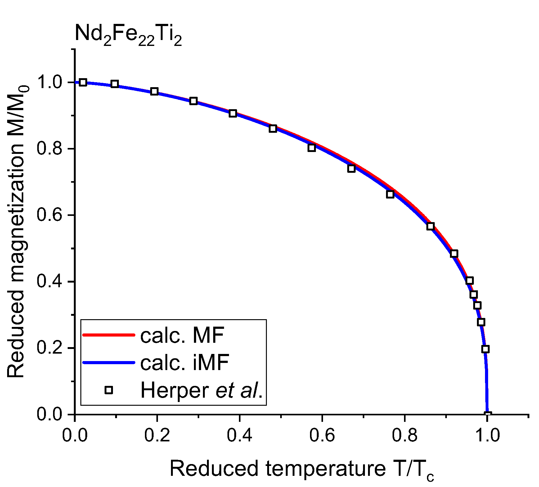
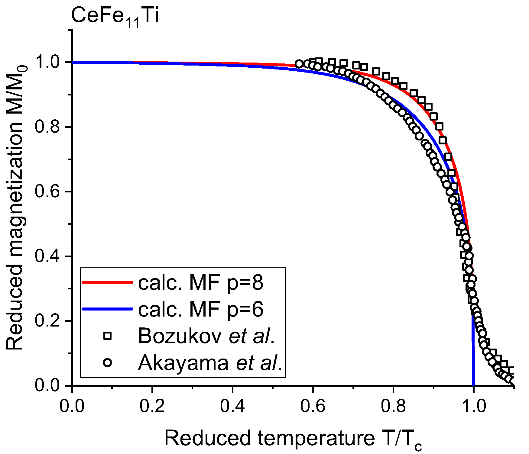
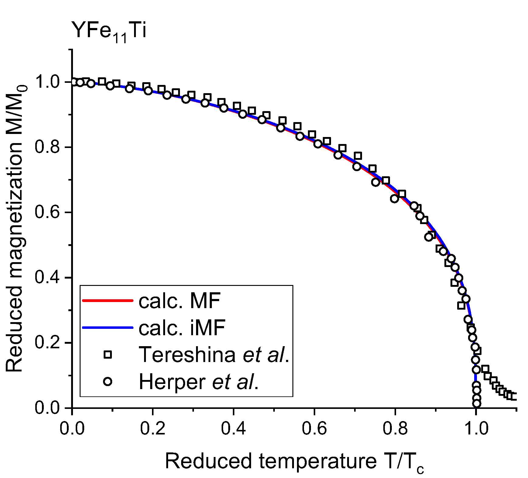
5.7 Magnetocrystalline Anisotropy
Magnetocrystalline anisotropy (MCA) is a critical magnetic property and must be addressed for a material once it has been tended to be used as a permanent magnet. Therefore, as the last intrinsic property, the magnetocrystalline anisotropy, which has a key importance for the performance of hard magnets is investigated. The MCA can be calculated by employing the magnetic force theorem [109] and by total energy differences. In this study, the latter one has been considered and magnetocrystalline anisotropy energy (MAE) is defined as
| (5.4) |
where and are the total energies of the considered supercells for the magnetization being oriented along the [110] and [001] directions, respectively.
For MAE calculations, the orientation of the magnetization along the crystallographic directions plays an important role. In Fig. 5.8, the resulting energy differences on basis of DFT and DFT+U calculations for changes from the easy magnetization axis [001] to the directions [110] and [010] are shown. DFT+U treatment leads to an increase of the energies of MJ/m3 for the clean and 0.1 to 0.2 MJ/m3 for the nitrogenated case. The influence of interstitial nitrogenation is depicted with the change from circles to squares with an energy increase of 0.4 MJ/m3. For the different direction changes from [001] to [110] and [001] and [010], shown in black and red, respectively, a significant energy difference of MJ/m3 is visible. Due to the higher energy difference, the change to [110] is mainly focused on in this work.


Based on the calculated magnetocrystalline anisotropy energy one can find the anisotropy constant and the anisotropy field . The anisotropy energy can be written as an expansion whose leading term is [10]
| (5.5) |
where is the angle between the magnetization direction and the easy axis. Further terms in the expansion reflect the crystal symmetry, but for many purposes, it is enough to consider only the leading term. A positive (negative) value corresponds to uniaxial (planar) anisotropy.
The anisotropy field is the upper limit for the coercivity and can be estimated from [10]
| (5.6) |
is an important property for permanent magnets, and a high value is needed for hard magnetic applications. Nevertheless, it must be noted that the calculated and values correspond to 0 K, therefore, the dependence of is excluded.
The calculated magnetocrystalline anisotropy constant and anisotropy field are given in Tab. 5.3 for the clean compounds. As listed, all the considered 1:12 phases have uniaxial anisotropy (>0). This linearity yields that higher-order anisotropy constants are negligible. We have examined our considered compounds and find that is almost 2 orders in magnitude smaller than the lowest order anisotropy constant, , which makes it sufficient to describe the MCA (for more details regarding the anisotropy constants see Ref. [91]).
| Alloy |
|
|
|
|
|
| ||||||||||||||||||||
| Y2Fe23Ti | 0.81 | 1.65 | 0.98 | 2.28 | ||||||||||||||||||||||
| Y2Fe22Ti2 | 0.92 | 1.73 |
|
1.22 | 2.76 |
| ||||||||||||||||||||
| Ce2Fe23Ti | 1.67 | 1.91 | 2.08 | 2.70 | ||||||||||||||||||||||
| Ce2Fe22Ti2 | 2.08 | 2.12 |
|
2.88 | 3.40 |
| ||||||||||||||||||||
| Nd2Fe23Ti |
|
1.32 |
|
2.12 | ||||||||||||||||||||||
| Nd2Fe22Ti2 |
|
1.41 |
|
|
2.57 |
| ||||||||||||||||||||
| NdYFe23Ti |
|
1.53 |
|
2.28 | ||||||||||||||||||||||
| NdYFe22Ti2 |
|
1.65 |
|
2.75 | ||||||||||||||||||||||
| NdCeFe23Ti |
|
1.43 |
|
2.13 | ||||||||||||||||||||||
| NdCeFe22Ti2 |
|
1.61 |
|
2.71 | ||||||||||||||||||||||
| Nd2Fe14B | 4.9j [11] | |||||||||||||||||||||||||
| Sm2Co17 | 4.2j [11] | |||||||||||||||||||||||||
| SmCo5 | 17.0j [11] | |||||||||||||||||||||||||
| Alnico 5 | 0.32j [11] |
- •
Theoretical references are represented by *
- •
a Mössbauer measurement at 300 K, b Mössbauer measurement at 77 K, c Mössbauer measurement at 4.2 K, d Single Crystal, Physical Property Measurement System (PPMS) measured at 10 K, e Derived from magnetization curve at 300 K, f Derived from magnetization curve at 4.2 K, g Determined by Kerr microscopy at 300 K, h X-ray diffraction measurement at 300 K, i X-ray diffraction measurement at 1.5 K, j Properties measured at 300 K.
As given in Tab. 5.3, an increasing Ti concentration also increases the anisotropy constant. Since periodic boundary conditions are used, the presence of Ti can be an artifact in an unevenly distributed small supercell. The missing real random distribution of Fe/Ti at 8i site also results in slightly non-equivalent basal directions [100] and [010].
In the case of YFe11Ti, the DFT (GGA) approximation yields the anisotropy constant as 0.92 MJ/m3. This is a clear underestimation of low temperature experimental values reported in the range of 1.89-2.1 MJ/m3 [114, 80, 95, 75]. In addition, a DFT based underestimated MCA is also reported by Ke et al. [85] and Herper et al. [75]. Therefore, the MCA is further examined by using LSDA. Significant improvement is achieved by using LSDA with 1.73 MJ/m3, which agrees better to experimental data.
The GGA results for CeFe11Ti already yield a very promising against experimental data. Known reported experimental values are ranging from 1.4 to 4.3 MJ/m3 [79, 81] based on the measurement technique and temperature. Nevertheless, the calculated with 2.08 MJ/m3 fits well to these experiments. The LSDA treatment for Ce-based compounds does not have a significant impact, and the is calculated to be 2.12 MJ/m3.
As mentioned earlier, 4f-electrons treatment in general DFT is not straightforward and based on the choice of the 4f localization MCA can yield different results. According to DFT (GGA) calculations in this study, where f-electrons are treated in core and no hybridization takes place between 4f and valence states, the anisotropy constant is calculated to be 0.54 MJ/m3 for the NdFe11Ti compound. Once we reduce the level of localization by applying the Hubbard U correction to the on-site Coulomb interactions is predicted to be 0.61 MJ/m3 for U=6 eV. In comparison to the experimental value of 1.78 MJ/m3 [75], both cases underestimates the MCA. As in the case of Y-based compounds, the LSDA treatment for NdFe11Ti yields better MCA results with respect to an experimental value of 1.41 MJ/m3.
According to the calculations in this work, both Y and Ce substitutions have improved the MCA compared to the NdFe11Ti case. In case of Y substituted 1:12 phase (Nd,Y)Fe11Ti, GGA (GGA+U) has a value of 0.74 (0.91) MJ/m3 and it is further improved for the Ce substituted case in (Nd,Ce)Fe11Ti with 1.27 (1.35) MJ/m3. Although, the GGA based calculations underestimate the MCA of NdFe11Ti with respect to measurements, it is known that experimentally reported YFe11Ti and CeFe11Ti values (1.89 [114] and 2 MJ/m3 [111]) are higher than the corresponding to NdFe11Ti (1.78 MJ/m3 [75]). Therefore, such a theoretical increase is accurately captured for both GGA (GGA+U) and LSDA calculations. In addition, for all considered compounds MCA is found to be uniaxial (>0) independently from the choice of exchange-correlation functionals, although GGA calculations for Y and Nd-based compounds strongly underestimate MCA. This is a good agreement with experimental data.
As given in Eq. 5.6, the anisotropy field can be calculated in a combination of the anisotropy constant and the saturation magnetization . In addition, as in the case of there is only available experimental data for the ternary compounds. In the case of the YFe11Ti compound the GGA calculations yield 1.22 T, which underestimates the low-temperature experimental values, reported to be in the range of 4.1 to 5.7 T [110, 94], and room temperature experimental values ranging from 2.2 to 4.8 T [94, 110]. The LSDA treatment leads to a significant improvement with a calculated value of 2.76 T, although there is still a deviation compared to low-temperature experimental data.
The anisotropy field of the CeFe11Ti compound is already well described by the GGA calculations with a value of 2.88 T. The experimental findings are reported in the range of 1.5 to 3.5 T [87, 112, 81] based on measurement technique and temperature. LSDA treatment yields a slightly higher value of 3.40 T, which also fits into the range of the reported experimental values and is near the value of 3.5 T measured by Pan et al. [87] with X-ray diffraction at 1.5 K. Therefore, the LSDA treatment does not have a significant impact as in the case of the Y and Nd-based ternaries.
In the NdFe11Ti calculations, the DFT (GGA) approach, with 4f-electrons treated as in core and no hybridization taking place, a value of 0.74 T is calculated. Applying the Hubbard U correction to the on-site Coulomb interactions the result increases to 0.96 T for U=6 eV. Comparing these results to the experimental findings of 1.9 T by Bouzidi et al. [113] and 2.0 T by Akayama et al. [81], a clear underestimation of our calculations is observed. Nevertheless, the LSDA treatment leads to an significant increase with 2.57 T, which better agrees with the reported experimental values.
In the case of quaternaries, the partial Nd substitution leads to an improvement for compared to NdFe11Ti ternary. For the Y substituted 1:12 compound NdYFe22Ti2 GGA (GGA+U), calculations result in a value of 1.0 (1.31) T. In the case of Ce substitution NdCeFe22Ti2, the increase is even larger with a value of 1.75 (2.00) T. As shown before, the LSDA treatment yields larger values for Y and Ce substituted quaternaries with 2.75 and 2.71 T, respectively. Since there are no experimental values to compare the theoretical findings of this work with for the considered quaternaries, it can only be deduced that the calculated values for the ternaries have a good agreement with experiments which is encouraging for the quaternary findings.

The calculated influence of interstitial nitrogenation on and for our GGA and GGA+U calculations is shown in Fig. 5.9. A general trend of an increase for and due to the addition of N is visible for all compounds. For instance, calculated via DFT for the Y-based ternary compound YFe11Ti is improved by 0.60 MJ/m3 to a value of 1.52 MJ/m3.
In case of the CeFe11Ti compound, the calculated value of 2.08 MJ/m3 for the clean case is raised by N doping to a result of 2.52 MJ/m3. The anisotropy field is consequently also increased due to nitrogenation to 3.36 T.
For NdFe11Ti the nitrogenated value is computed with DFT (DFT+U) to be 0.92 (1.0) MJ/m3. The according result for is calculated as 0.96 (1.47) T.
The impact of N on the quarternary compounds NdYFe22Ti2 NdCeFe22Ti2 is similar to the ternary ones. For , an increase from 0.74 (0.91) to 1.21 (1.27) MJ/m3 and 1.27 (1.35) to 1.72 (1.78) MJ/m3 for the respective compounds is observed. Since the calculation of the anisotropy field is based on the anisotropy constant, the increasement of leads to an improvement of the anisotropy field up to values of 1.56 (1.75) and 2.26 (2.52) T, respectively.
For all considered compounds, an average increase of MJ/m3 due to the additon of N atoms into the 2b site can be recorded. The biggest individual increase is seen for the above mentioned YFe11Ti compound with an improvement of 0.60 MJ/m3.
5.8 Hardness Factor
From the first-principles calculations, the magnetic hardness factor can be evaluated from the expression of saturation magnetisation and magnetocrystalline anisotropy constant by
| (5.7) |
This parameter indicates the potential for a material to be developed into a permanent magnet independently of the shape when >1. In addition, a material can be considered as a semi-hard (0.1 << 1) and soft magnet (<0.1) accordingly [11].
The calculated magnetic hardness factors are depicted in Fig. 5.10 for both GGA (GGA+U) and LSDA functionals. As mentioned above, for Y and Nd-based compounds, a better agreement with respect to experimental data by LSDA calculations was achieved. Therefore, LSDA based values are more reliable, and it is noticeable that for all considered compounds >1. Herper et al. [75] calculated the magnetic hardness factor for YFe11Ti for both GGA and LSDA and found =0.63 and 1.23, respectively. This agrees with the calculated values in this work, which are 0.71 (GGA) and 1.18 (LSDA), respectively.
For CeFe11.5Ti0.5 and CeFe11Ti Snarsky-Adamsky et al. [97] reported theoretical values, calculated using the full-potential local-orbital code from 2018 (FPLO18) with the PBE functional, of 0.52 and 0.79 respectively. While these values are slightly smaller than the GGA results of 0.90 and 1.12 in this study, the trend of an increasing hardness factor with an increase of Ti concentration is in good agreement.
In case of Y and Ce substituted Nd-based 1:12 phases, promising values for LSDA treatment are observed. For both NdYFe22Ti2 and NdCeFe22Ti2 cases the calculated value is =1.20. Note that the value for the commonly used Nd2Fe14B magnet is reported to be 1.54 [11]. In the considered benchmark system of this thesis, by considering 50% Nd-lean quaternaries, a very close magnetic hardness factor with respect to the market leading hard magnet was reached which is technologically encouraging.

Chapter 6 Conclusion and Outlook
In conclusion, based on the promising finite temperature phase stability findings for Nd-lean permanent magnets [35], systematic investigations on the intrinsic magnetic properties for (Nd,X)Fe12-yTiy compounds have been performed. As an alternative element to substitute critical Nd, abundant and inexpensive elements, X= Y and Ce, have been chosen. Since there is no experimental data for the considered quaternary compounds in the literature, only the theoretical results for ternary compounds could be compared and a promising agreement could be seen. This gives a strong confidence in the calculated magnetic properties of Nd-lean quaternaries.
An accurate description of RE 4f-electrons has critical importance for a successful prediction of intrinsic magnetic properties. Due to the strong hybridization of Ce-4f with TM-3d-electrons, in addition to previous works by Sözen et al. [7, 52, 53, 35], conventional DFT calculations are performed for Ce-based compounds and yield satisfactory results. However, Nd 4f-electrons are strongly localized and available DFT exchange-correlation functionals have difficulties to accurately capture this property. Therefore, as a correction scheme, the DFT+U approach with Hubbard U=6 eV has been used.
The methodology of this work perfectly predicts the total magnetization trend of the 1:12 phases, that NdFe11Ti has the highest magnetisation and is followed by YFe11Ti and CeFe11Ti. Experimentally reported saturation magnetisation for NdFe11Ti is deviating from 1.38 to 1.70 T [86, 89, 75, 81] based on the measurement temperature and method. Our DFT (DFT+U) calculations yield 1.47 (1.28) T, which is a good agreement. In the case of Y and Ce substitution is found to be 1.49 (1.39) T for NdYFe22Ti2 and 1.46 (1.35) T for NdCeFe22Ti2 based on DFT (DFT+U). In addition, for all considered compounds further improvement by 0.1 T is achieved after nitrogenation and it is found that the magnetovolume effect plays a major role rather than chemical effects. Based on the magnetisation calculations, very high |BH|max values for NdYFe22Ti2 and NdCeFe22Ti2 were achieved, which are 384 and 365 kJ/m3, and they are higher than the |BH|max of Sm2Co17B, 294 kJ/m3 [10]. Note that, lower Ti contained quaternaries, NdYFe23Ti (484 kJ/m3) and NdCeFe23Ti (466 kJ/m3), have close |BH|max values to the Nd2Fe14B magnet that exhibits 512 kJ/m3 [10]. In addition, a further increase of |BH|max values around 40 kJ/m3 is calculated with nitrogenation.
Curie temperatures are calculated by the mean-field approximation (MFA). Systematic overestimation of for ferromagnetic (FM) state calculations is observed. Nevertheless, quantitative agreement of decreasing for increasing Ti concentration and increasing after nitrogenation is captured with respect to experimental data. Miyake et al. [105] reported that local moment disorder (LMD) calculations yield better performance for the of REFe11Ti compounds. Our LMD calculations agree with this finding. In the case of YFe11Ti, CeFe11Ti and NdFe11Ti, the LMD-based calculations overestimate the experimental data by 9, 12 and 20 %, respectively. Note that, in the case of FM-based calculations, the margin of error is around 45% for these ternaries. The LMD calculations yield 595 and 593 K values for the Nd-lean quaternaries NdYFe22Ti2 and NdCeFe22Ti2, respectively. For both cases, theoretical is slightly higher than the experimental of Nd2Fe14B, which is 588 K.
In the case of the magnetocrystalline anisotropy constant , the generalized gradient approximation (GGA) based exchange-correlation functional failed for Y and Nd-based compounds. The shortcomings of GGA is also reported for such compounds by Herper et al. and Ke et al. [75, 85]. Therefore, the local spin density approximation (LSDA) was further considered and reached a better agreement with respect to the experiment. Knowing and allows to calculate the magnetic hardness factor , which relates to the potential of a material to be developed into a permanent magnet and >1 is desired. Our 50% Nd-lean quaternaries yield a 1.20 theoretical value which is close to the magnetic hardness factor of 1.54 for Nd2Fe14B.
As a conclusion to this thesis, it was shown that the substitution of critical RE elements, such as Nd, in compounds of the ThMn12 structure with more available elements like Ce or Y yields possible alternatives to the RE-TM type Nd-Fe-B magnets with comparable or only slightly smaller magnetic properties. These new quarternary (NdX)Fe24-yTiy (X=Y or Ce) compounds can consequently be considered as an achievable way to produce more affordable magnets with a smaller amount of critically labeled elements. As an outlook to this work, the further investigation of other elements, besides Ce and Y, with a combination of DFT and KKR calculations for the substitution with the Nd-atoms can be considered. Another possibility would be the expansion to other known magnetic structures such as the 2:14 or 2:17 phases and research the possible reduction of RE-elements in these compounds as well. Due to similar s the investigated quarternary compounds are very appealing in a technological perspective as they could be used in almost the same field of applications as the Nd-Fe-B magnets when slightly lower magnetic properties are still acceptable.
References
- [1] O. Gutfleisch, M. A. Willard, E. Brück, C. H. Chen, S. G. Sankar, and J. P. Liu, “Magnetic materials and devices for the 21st century: Stronger, lighter, and more energy efficient,” Advanced Materials, vol. 23, no. 7, pp. 821–842, 2011.
- [2] K. P. Skokov and O. Gutfleisch, “Heavy rare earth free, free rare earth and rare earth free magnets - Vision and reality,” Scripta Materialia, vol. 154, pp. 289–294, 2018.
- [3] I. Poenaru, A. Lixandru, S. Riegg, B. Fayyazi, A. Taubel, K. Güth, R. Gauß, and O. Gutfleisch, “Ce and La as substitutes for Nd in Nd2Fe14B-based melt-spun alloys and hot-deformed magnets: a comparison of structural and magnetic properties,” Journal of Magnetism and Magnetic Materials, vol. 478, pp. 198–205, 2019.
- [4] J. M. Coey, Magnetism and Magnetic Materials. Cambridge U.K.: Cambridge University Press, 2009.
- [5] P. M. Levy and E. W. Lee, Magnetism: An introductory survey. Pergamon Press, New York, 6 ed., 1973.
- [6] B. Cullity and C. Graham, Introduction to Magnetic Materials. Hoboken, New Jersey: Wiley, IEEE Press, 2 ed., 2009.
- [7] H. I. Sözen, Ab initio phase stabilities of Ce-based hard magnetic materials. Ph.d. thesis, Ruhr-Universität Bochum, 2019.
- [8] FZ-Jülich, “https://aiida-fleur.readthedocs.io/en/v1.1.1/user_guide/ workflows/ mae_conv_wc.html.”
- [9] H. S. Li and J. M. Coey, “Magnetic properties of ternary rare-earth transition-metal compounds,” Handbook of Magnetic Materials, vol. 28, pp. 87–196, 2019.
- [10] J. M. Coey, “Hard magnetic materials: A perspective,” IEEE Transactions on Magnetics, vol. 47, no. 12, pp. 4671–4681, 2011.
- [11] R. Skomski and J. M. Coey, “Magnetic anisotropy - How much is enough for a permanent magnet?,” Scripta Materialia, vol. 112, pp. 3–8, 2016.
- [12] S. M. Abdelbasir and A. E. Shalan, Intriguing Properties and Applications of Functional Magnetic Materials. IntechOpen, 2019.
- [13] W. C. Ellis and E. E. Schumacher, “A Survey of Magnetic Materials in Relation to Structure,” Bell System Technical Journal, vol. 14, no. 1, pp. 8–43, 1935.
- [14] R. A. McCurrie, “The structure and properties of alnico permanent magnet alloys,” Ferromagnetic Materials, vol. 3, pp. 107–109, 111–188, 1982.
- [15] É. Trémolet de Lacheisserie, D. Gignoux, and M. Schlenker, Magnetism: Materials and Applications. New-York: Springer-Verlag, 1 ed., 2005.
- [16] M. Sugimoto, “The Past, Present, and Future of Ferrites,” Journal of the American Ceramic Society, vol. 82, no. 2, pp. 269–280, 1999.
- [17] J. M. Coey, “Perspective and Prospects for Rare Earth Permanent Magnets,” Engineering, vol. 6, no. 2, pp. 119–131, 2020.
- [18] K. J. Strnat and K. D. Hoffer, “YCo5, A Promising New Permanent Magnetic Material,” tech. rep., Technical Report, Air Force Report AFML-TR-65-446, 1966.
- [19] M. Sagawa, S. Fujimura, and N. Togawa, “New material for permanent magnets on a base of Nd and Fe,” Journal of Applied Physics, vol. 55, p. 2083, 1984.
- [20] J. J. Croat, J. F. Herbst, R. W. Lee, and F. E. Pinkerton, “Pr-Fe and Nd-Fe-based materials: A new class of high-performance permanent magnets (invited),” Journal of Applied Physics, vol. 55, no. 6, pp. 2078–2082, 1984.
- [21] J. Cui, J. Ormerod, D. Parker, R. Ott, A. Palasyuk, S. Mccall, M. P. Paranthaman, M. S. Kesler, M. A. McGuire, I. C. Nlebedim, C. Pan, and T. Lograsso, “Manufacturing Processes for Permanent Magnets: Part I—Sintering and Casting,” Jom, vol. 74, no. 4, pp. 1279–1295, 2022.
- [22] S. Magnets, “https://www.stanfordmagnets.com/development-of-the-ndfeb-magnet-industry.html.”
- [23] D. J. Cordier, “Mineral Commodity Summaries,” tech. rep., U.S. Geological Survey (USGS), 2022.
- [24] D. Bauer, D. Diamond, J. Li, M. McKittrick, D. Sandalow, and P. Telleen, “Critical Materials Strategy for Clean Energy Technologies,” US Department of Energy Office of Policy and International Affairs (PI), pp. 1–170, 2011.
- [25] M. Pellegrini, “Report on Critical Raw Materials for the EU,” tech. rep., 2014.
- [26] H. Sepehri-Amin, Y. Une, T. Ohkubo, K. Hono, and M. Sagawa, “Microstructure of fine-grained Nd-Fe-B sintered magnets with high coercivity,” Scripta Materialia, vol. 65, no. 5, pp. 396–399, 2011.
- [27] K. Hono and H. Sepehri-Amin, “Strategy for high-coercivity Nd-Fe-B magnets,” Scripta Materialia, vol. 67, no. 6, pp. 530–535, 2012.
- [28] W. F. Li, T. Ohkubo, T. Akiya, H. Kato, and K. Hono, “The role of Cu addition in the coercivity enhancement of sintered Nd-Fe-B permanent magnets,” Journal of Materials Research, vol. 24, no. 2, pp. 413–420, 2009.
- [29] H. Sepehri-Amin, T. Ohkubo, S. Nagashima, M. Yano, T. Shoji, A. Kato, T. Schrefl, and K. Hono, “High-coercivity ultrafine-grained anisotropic Nd-Fe-B magnets processed by hot deformation and the Nd-Cu grain boundary diffusion process,” Acta Materialia, vol. 61, no. 17, pp. 6622–6634, 2013.
- [30] Z. B. Li, B. G. Shen, M. Zhang, F. X. Hu, and J. R. Sun, “Substitution of Ce for Nd in preparing R2Fe14B nanocrystalline magnets,” Journal of Alloys and Compounds, vol. 628, pp. 325–328, 2015.
- [31] J. Jin, G. Bai, Z. Zhang, and M. Yan, “Coercivity enhancement for Nd-La-Ce-Fe-B sintered magnets by tailoring La and Ce distributions,” Journal of Alloys and Compounds, vol. 763, pp. 854–860, 2018.
- [32] D. D. Mooij and K. Buschow, “Some Novel Ternary ThMn12-type Compounds,” Journal of the Less-Common Metals, vol. 136, no. 2, pp. 207–215, 1988.
- [33] K. H. Buschow, “Permanent magnet materials based on tetragonal rare earth compounds of the type RFe12-xMx,” Journal of Magnetism and Magnetic Materials, vol. 100, no. 1-3, pp. 79–89, 1991.
- [34] A. M. Gabay and G. C. Hadjipanayis, “Recent developments in RFe12-type compounds for permanent magnets,” Scripta Materialia, vol. 154, pp. 284–288, 2018.
- [35] H. I. Sözen and T. Klüner, “Ab initio phase stabilities of rare-earth lean Nd-based hard magnets,” Journal of Magnetism and Magnetic Materials, vol. 559, pp. 1–20, 2022.
- [36] Y. Hirayama, Y. K. Takahashi, S. Hirosawa, and K. Hono, “NdFe12Nx hard-magnetic compound with high magnetization and anisotropy field,” Scripta Materialia, vol. 95, no. 1, pp. 70–72, 2015.
- [37] H. Suzuki, “Metastable phase YFe12 fabricated by rapid quenching method,” AIP Advances, vol. 7, no. 5, pp. 0–7, 2017.
- [38] Y. Hirayama, Y. K. Takahashi, S. Hirosawa, and K. Hono, “Scripta Materialia Intrinsic hard magnetic properties of Sm (Fe1-x Co x )12 compound with the ThMn12 structure,” Scripta Materialia, vol. 138, pp. 62–65, 2017.
- [39] P. Hohenberg and W. Kohn, “Inhomogeneous Electron Gas,” Physical Review, vol. 136, no. 3B, pp. B864–B871, 1964.
- [40] R. G. Parr and W. Yang, Density-Functional Theory of Atoms and Molecules. Oxford: Oxford University Press, 1989.
- [41] W. Koch and M. C. Holthausen, Wolfram Koch , Max C . Holthausen A Chemist ’ s Guide to. Wiley-VCH, 2 ed., 2001.
- [42] W. Kohn and L. Sham, “Self-Consistent Equations Including Exchange and Correlation Effects,” Physical Review, vol. 140, no. 4A, pp. A1133–A1138, 1965.
- [43] A. D. Becke, “Perspective: Fifty years of density-functional theory in chemical physics,” Journal of Chemical Physics, vol. 140, no. 18, 2014.
- [44] M. Dumaz, R. Boucher, M. A. Marques, and A. H. Romero, “Authorship and citation cultural nature in Density Functional Theory from solid state computational packages,” Scientometrics, vol. 126, pp. 6681–6695, 2021.
- [45] M. Born and R. Oppenheimer, “Zur Quantentheorie der Molekeln,” Annalen der Physik, vol. 20, no. 84, pp. 457–484, 1927.
- [46] J. P. Perdew and K. Schmidt, “Jacob’s ladder of density functional approximations for the exchange-correlation energy,” AIP Conf. Proc., vol. 577, no. 1, pp. 1–20, 2001.
- [47] E. Awoonor-Williams, “Brief Overview on Density Functional Theory,” 2018.
- [48] S. H. Vosko, L. Wilk, and M. Nusair, “Accurate spin-dependent electron liquid correlation energies for local spin density calculations: a critical analysis,” Canadian Journal of Physics, vol. 58, no. 8, pp. 1200–1211, 1980.
- [49] J. P. Perdew, K. Burke, and M. Ernzerhof, “Generalized gradient approximation made simple,” Physical Review Letters, vol. 77, no. 18, pp. 3865–3868, 1996.
- [50] J. P. Perdew and Y. Wang, “Accurate and simple analytic representation of the electron-gas correlation energy,” Physical Review B, vol. 45, no. 23, pp. 244–249, 1992.
- [51] J. P. Perdew, J. A. Chevary, S. H. Vosko, K. A. Jackson, M. R. Pederson, D. J. Singh, and C. Fiolhais, “Atoms, molecules, solids, and surfaces: Applications of the generalized gradient approximation for exchange and correlation,” Physical Review B, vol. 46, no. 11, pp. 6671–6687, 1992.
- [52] H. I. Sözen, S. Ener, F. Maccari, K. P. Skokov, O. Gutfleisch, F. Körmann, J. Neugebauer, and T. Hickel, “Ab initio phase stabilities of Ce-based hard magnetic materials and comparison with experimental phase diagrams,” Physical Review Materials, vol. 3, no. 8, pp. 1–15, 2019.
- [53] H. I. Sözen, T. Hickel, and J. Neugebauer, “Impact of magnetism on the phase stability of rare-earth based hard magnetic materials,” Calphad: Computer Coupling of Phase Diagrams and Thermochemistry, vol. 68, no. December 2019, 2020.
- [54] P. E. Blöchl, “Projector augmented-wave method,” Physical Review B, vol. 50, no. 24, pp. 17953–17979, 1994.
- [55] G. Kresse and D. Joubert, “From ultrasoft pseudopotentials to the projector augmented-wave method,” Physical Review B - Condensed Matter and Materials Physics, vol. 59, no. 3, pp. 1758–1775, 1999.
- [56] D. Vanderbilt, “Soft self-consistent pseudopotentials in a generalized eigenvalue formalism,” Rapid Communications, vol. 41, no. 11, pp. 7892–7895, 1990.
- [57] K. W. Böer and U. W. Pohl, Semiconductor Physics. Cham: Springer, 2018.
- [58] U. Von Barth and L. Hedin, “A local exchange-correlation potential for the spin polarized case. I,” Journal of Physics C: Solid State Physics, vol. 5, no. 13, pp. 1629–1642, 1972.
- [59] G. Bihlmayer, “Density-functional Theory of Magnetism,” in Handbook of Magnetism and Advanced Magnetic Materials (H. Kronmüller and S. Parkin, eds.), Wiley, 2007.
- [60] A. I. Lichtenstein, V. Anisimov, and J. Zaanen, “Density-functional theory and strong interactions: Orbital ordering in Mott-Hubbard insulators,” Physical Review B, vol. 52, no. 8, pp. 5467–5471, 1995.
- [61] S. Dudarev and G. Botton, “Electron-energy-loss spectra and the structural stability of nickel oxide: An LSDA+U study,” Physical Review B - Condensed Matter and Materials Physics, vol. 57, no. 3, pp. 1505–1509, 1998.
- [62] A. Georges and G. Kotliar, “Hubbard model in infinite dimensions,” Physical Review B, vol. 45, no. 12, pp. 6479–6483, 1992.
- [63] A. Liechtenstein, M. Katsnelson, V. Antropov, and V. Gubanov, “Local Spin Density Functional Approach to the Theory of Exchange Interactions in Ferromagnetic Metals and Alloys,” Journal of Magnetism and Magnetic Materials, vol. 67, pp. 65–74, 1987.
- [64] G. Kresse and J. Furthmüller, “Efficiency of ab-initio total energy calculations for metals and semiconductors using a plane-wave basis set,” Computational Materials Science, vol. 6, no. 1, pp. 15–50, 1996.
- [65] G. Kresse and J. Furthmüller, “Efficient iterative schemes for ab initio total-energy calculations using a plane-wave basis set,” Physical Review B - Condensed Matter and Materials Physics, vol. 54, no. 16, pp. 11169–11186, 1996.
- [66] J. Korringa, “On the Calculation of the Energy of a Bloch Wave in a Metal,” Physica, no. 6, pp. 392–400, 1947.
- [67] W. Kohn and N. Rostoker, “Solution of the schrödinger equation in periodic lattices with an application to metallic lithium,” Physical Review, vol. 94, no. 5, pp. 1111–1120, 1954.
- [68] H. Akai, “http://kkr.issp.u-tokyo.ac.jp.”
- [69] H. Shiba, “A Reformulation of the Coherent Potential Approximation and Its Applications,” Progress of Theoretical Physics, vol. 46, no. 1, pp. 77–94, 1971.
- [70] H. Akai, “Residual resistivity of Ni-Fe, Ni-Cr and other ferromagnetic alloys,” Physica B+C, vol. 86-88, no. 1, pp. 539–540, 1977.
- [71] A. W. V.L. Moruzzi, J.F. Janak, Calculated Properties of Metals. Pergamon Press, New York, 1978.
- [72] J. Jensen and A. R. Mackintosh, “Rare earth magnetism: structures and excitations,” Physics, p. 403, 1991.
- [73] M. Richter, “Band structure theory of magnetism in 3d-4f compounds,” Journal of Physics D: Applied Physics, vol. 31, no. 9, pp. 1017–1048, 1998.
- [74] J. K. Lang, P. A. Cox, and Y. Baer, “Study of the 4f and valence band density of states in rare-earth metals. I. Theory of the 4f states,” Journal of Physics F: Metal Physics, vol. 11, no. 1, pp. 113–119, 1981.
- [75] H. C. Herper, K. Skokov, S. Ener, P. Thunström, L. V. B. Diop, O. Gutfleisch, and O. Eriksson, “Magnetic Properties of NdFe11Ti and YFe11Ti, from Experiment and Theory,” SSRN Electronic Journal, 2022.
- [76] N. Drebov, A. Martinez-Limia, L. Kunz, A. Gola, T. Shigematsu, T. Eckl, P. Gumbsch, and C. Elsässer, “Ab initio screening methodology applied to the search for new permanent magnetic materials,” New Journal of Physics, vol. 15, 2013.
- [77] W. Körner, G. Krugel, and C. Elsässer, “Theoretical screening of intermetallic ThMn12 -type phases for new hard-magnetic compounds with low rare earth content,” Scientific Reports, vol. 6, no. February, pp. 1–9, 2016.
- [78] I. Dirba, Y. Harashima, H. Sepehri-Amin, T. Ohkubo, T. Miyake, S. Hirosawa, and K. Hono, “Thermal decomposition of ThMn12-type phase and its optimum stabilizing elements in SmFe12-based alloys,” Journal of Alloys and Compounds, vol. 813, p. 152224, 2020.
- [79] O. Isnard, S. Miraglia, M. Guillot, and D. Fruchart, “Hydrogen effects on the magnetic properties of RFe11Ti compounds,” Journal of Alloys and Compounds, vol. 275-277, pp. 637–641, 1998.
- [80] I. S. Tereshina, P. Gaczynski, V. S. Rusakov, H. Drulis, S. A. Nikitin, W. Suski, N. V. Tristan, and T. Palewski, “Magnetic anisotropy and Mössbauer effect studies of YFe11Ti and YFe11TiH,” Journal of Physics: Condensed Matter, vol. 13, p. 8161, 2001.
- [81] M. Akayama, H. Fujii, K. Yamamoto, and K. Tatami, “Physical properties of nitrogenated RFe11Ti intermetallic compounds (R=Ce, Pr and Nd) with ThMn12-type structure,” Journal of Magnetism and Magnetic Materials, vol. 130, no. 1-3, pp. 99–107, 1994.
- [82] K. Buschow, Electronic and Magnetic Properties of Metals and Ceramics, Part II, Materials Science and Technology Series. VCH, 3b ed., 1994.
- [83] O. Isnard, Role of interstitial elements on permanent magnet alloys based on rare earth elements and iron: Synthesis, structural study, spectroscopic analysis in relation to magnetic properties. Ph.d. thesis, University Grenoble, 1993.
- [84] Y. Wang, J. Shen, N. X. Chen, and J. L. Wang, “Theoretical investigation on site preference of foreign atoms in rare-earth intermetallics,” Journal of Alloys and Compounds, vol. 319, no. 1-2, pp. 62–73, 2001.
- [85] L. Ke and D. D. Johnson, “Intrinsic magnetic properties in R(Fe1-xCox)11TiZ (R= Yand Ce;Z= H,C,and N),” Physical Review B, vol. 94, no. 2, pp. 1–9, 2016.
- [86] Y. C. Yang, X. D. Zhang, S. L. Ge, Q. Pan, L. S. Kong, H. Li, J. L. Yang, B. S. Zhang, Y. F. Ding, and C. T. Ye, “Magnetic and crystallographic properties of novel Fe-rich rare-earth nitrides of the type RTiFe11N1-δ (invited),” Journal of Applied Physics, vol. 70, no. 10, pp. 6001–6005, 1991.
- [87] Q. Pan, Z.-x. Liu, and Y.-c. Yang, “Structural and magnetic properties of Ce (Fe ,M )Nx interstitial compounds, M=Ti, V, Cr, and Mo,” Journal of Applied Physics, vol. 76, pp. 6728–6730, 1994.
- [88] Y. Hirayama, T. Miyake, and K. Hono, “Rare-Earth Lean Hard Magnet Compound NdFe12N,” Jom, vol. 67, no. 6, pp. 1344–1349, 2015.
- [89] C. Piquer, F. Grandjean, O. Isnard, V. Pop, and G. J. Long, “A magnetic and Mössbauer spectral study of the spin reorientation in NdFe11Ti and NdFe11TiH,” Journal of Applied Physics, vol. 95, no. 11 I, pp. 6308–6316, 2004.
- [90] S. Suzuki, T. Kuno, K. Urushibata, K. Kobayashi, N. Sakuma, K. Washio, H. Kishimoto, A. Kato, and A. Manabe, “A (Nd, Zr)(Fe, Co)11.5Ti0.5Nx compound as a permanent magnet material,” AIP Advances, vol. 4, no. 11, pp. 7–12, 2014.
- [91] S. A. Nikitin, I. S. Tereshina, V. N. Verbetskiǐ, and A. A. Salamova, “Magnetic anisotropy of YFe11Ti and its hydride,” Physics of the Solid State, vol. 40, no. 2, pp. 258–262, 1998.
- [92] Y. chang Yang, X. dong Zhang, L. shu Kong, Q. Pan, and S. lin Ge, “New potential hard magnetic material - NdTiFe11Nx,” Solid State Communications, vol. 78, no. 4, pp. 317–320, 1991.
- [93] A. Vishina, O. Eriksson, O. Y. Vekilova, A. Bergman, and H. C. Herper, “Ab-initio study of the electronic structure and magnetic properties of Ce2Fe17,” Journal of Alloys and Compounds, vol. 888, p. 161521, 2021.
- [94] S. Obbade, D. Fruchart, M. Bououdina, S. Miraglia, J. L. Soubeyroux, and O. Isnard, “About hydrogen insertion in ThMn12 type alloys,” Journal of Alloys and Compounds, vol. 253-254, pp. 298–301, 1997.
- [95] Q. N. Qi, Y. P. Li, and J. M. Coey, “Gas-phase interstitially modified intermetallics R(Fe11Ti) Z1-delta: II. 3d magnetization of the compounds Y(Fe11Ti) Z1-delta (Z = N, C),” Journal of Physics: Condensed Matter, vol. 4, no. 42, pp. 8209–8220, 1992.
- [96] W. Mao, J. Yang, B. Cui, B. Cheng, Y. Yang, H. Du, B. Zhang, C. Ye, and J. Yang, “A study on the effect of hydrogen in the compounds with ThMn12-type structure,” Journal of Physics Condensed Matter, vol. 10, no. 12, pp. 2611–2616, 1998.
- [97] J. Snarski-Adamski and M. Werwiński, “Effect of transition metal doping on magnetic hardness of CeFe12-based compounds,” Journal of Magnetism and Magnetic Materials, vol. 554, no. July, 2022.
- [98] T. Fukazawa, H. Akai, Y. Harashima, and T. Miyake, “First-principles investigation of Nd(Fe,M)12 (M = K–Br) and Nd(Fe,Cr,Co,Ni,Ge,As)12: Possible enhancers of Curie temperature for NdFe12 magnetic compounds,” Acta Materialia, vol. 226, 2022.
- [99] Y. Harashima, K. Terakura, H. Kino, S. Ishibashi, and T. Miyake, “Nitrogen as the best interstitial dopant among X= B, C, N, O, and F for strong permanent magnet NdFe11TiX: First-principles study,” Physical Review B - Condensed Matter and Materials Physics, vol. 92, no. 18, pp. 1–13, 2015.
- [100] R. Skomski, Simple Models of Magnetism. Oxford University Press on Demand, 2008.
- [101] J. Fidler, T. Schrefl, S. Hoefinger, and M. Hajduga, “Recent developments in hard magnetic bulk materials,” Journal of Physics Condensed Matter, vol. 16, no. 5, 2004.
- [102] H. Akai and P. H. Dederichs, “Local moment disorder in ferromagnetic alloys,” Physical Review B, vol. 47, no. 14, pp. 8739–8747, 1993.
- [103] B. L. Gyorffy, A. J. Pindor, J. Staunton, G. M. Stocks, and H. Winter, “A first-principles theory of ferromagnetic phase transitions in metals,” Journal of Physics F: Metal Physics, vol. 15, no. 6, pp. 1337–1386, 1985.
- [104] F. Maccari, S. Ener, D. Koch, I. Dirba, K. P. Skokov, E. Bruder, L. Schäfer, and O. Gutfleisch, “Correlating changes of the unit cell parameters and microstructure with magnetic properties in the CeFe11Ti compound,” Journal of Alloys and Compounds, vol. 867, p. 158805, 2021.
- [105] T. Miyake, Y. Harashima, T. Fukazawa, and H. Akai, “Understanding and optimization of hard magnetic compounds from first principles,” Science and Technology of Advanced Materials, vol. 22, no. 1, pp. 543–556, 2021.
- [106] M. D. Kuz’min, “Shape of temperature dependence of spontaneous magnetization of ferromagnets: Quantitative analysis,” Physical Review Letters, vol. 94, no. 10, pp. 16–19, 2005.
- [107] F. Körmann, A. Dick, B. Grabowski, B. Hallstedt, T. Hickel, and J. Neugebauer, “Free energy of bcc iron: Integrated ab initio derivation of vibrational, electronic, and magnetic contributions,” Physical Review B - Condensed Matter and Materials Physics, vol. 78, no. 3, pp. 1–4, 2008.
- [108] L. Bozukov, A. Apostolov, and M. Stoytchev, “A change in magnetic and structural properties of the CeFe11Ti intermetallic compound upon hydrogen absorption,” Journal of Magnetism and Magnetic Materials, vol. 101, no. 1-3, pp. 355–356, 1991.
- [109] M. Springford and D. Shoenberg, Electrons at the Fermi Surface. Cambridge U.K.: Cambridge University Press, 1980.
- [110] J. L. Wang, N. Tang, B. Fuquan, W. H. Wang, W. Q. Wang, G. H. Wu, and F. M. Yang, “Study of the magnetocrystalline anisotropy of RFe11-xCoxTi compounds with R = Y and Er,” Journal of Physics Condensed Matter, vol. 13, no. 8, pp. 1617–1626, 2000.
- [111] D. Goll, R. Loeffler, R. Stein, U. Pflanz, S. Goeb, R. Karimi, and G. Schneider, “Temperature dependent magnetic properties and application potential of intermetallic Fe11-xCoxTiCe,” Physica Status Solidi - Rapid Research Letters, vol. 8, no. 10, pp. 862–865, 2014.
- [112] C. Zhou, F. E. Pinkerton, and J. F. Herbst, “Magnetic properties of CeFe 11-xCoxTi with ThMn12 structure,” Journal of Applied Physics, vol. 115, no. 17, p. 17C716, 2014.
- [113] W. Bouzidi, T. Bartoli, R. Sedek, A. Bouzidi, J. Moscovici, and L. Bessais, “Low-field magnetocaloric effect of NdFe11Ti and SmFe10V2 compounds,” Journal of Materials Science: Materials in Electronics, vol. 32, no. 8, pp. 10579–10586, 2021.
- [114] S. A. Nikitin, I. S. Tereshina, V. N. Verbetsky, and A. A. Salamova, “Magnetic anisotropy of YFe11Ti single crystal and its hydride,” International Journal of Hydrogen Energy, vol. 24, no. 2, pp. 217–219, 1999.
List of Abbreviations
-
RE - Rare-earth
-
TM - Transition metal
-
- Total magnetic moment
-
- Magnetic constant
-
- Bohr magneton
-
- Magnetic field
-
- Anisotropy field
-
- Coercivity field
-
- Internal magnetic field
-
- Magnetization
-
- Remanence magnetization
-
- Magnetization saturation
-
- Finite temperature magnetization
-
- Reduced magnetization
-
- Curie temperature
-
|BH|max - Maximum energy product
-
MCA - Magnetocrystalline anisotropy
-
MAE - Magnetocrystalline anisotropy energy
-
- Anisotropy energy
-
- Anisotropy constant 1 order
-
- Hardness factor
-
HF - Hartree-Fock
-
post-HF - post Hartree-Fock
-
DFT - Density functional theory
-
DFT+U - Density functional theory with applied Hubbard U correction
-
DMFT - Dynamical mean field theory
-
LDA - Local Density Approximation
-
LSDA - Local Spin Density Approximation
-
GGA - Generalized Gradient Approximation
-
PW91 - Functional by Perdew and Wang
-
PBE - Functional by Perdew, Burke and Ernzerhof
-
PAW - Projector Augmented Wave
-
USPP - Ultrasoft Pseudopotentials
-
VASP - Vienna ab initio Simulation Package
-
KKR - Korringa-Kohn-Rostoker
-
SCF - self-consistent field
-
FM - Ferromagnetic
-
LMD - Local Moment Disorder
-
DLM - Disorder local moment
-
MFA - Mean-field approximation
-
ASA - Atomic sphere approximation
-
CPA - Coherent potential approximation
-
MJW - Moruzzi, Janak and Williams
-
TB-LMTO-ASA - Tight-binding linear-muffin-tin-orbital atomic-sphere-approximation
-
FPLO18 - Full potential local orbital code released in 2018
-
DOS - Density of states
-
XRD - X-Ray diffraction
-
ESM - Extraction sample magnetometer
-
PPMS - Physical property measurement system
-
VSM - Vibrating sample magnetometer
-
bcc - Body centered cubic
Erklärung
Hiermit versichere ich an Eides statt, dass ich diese Arbeit selbstständig verfasst und keine anderen als die angegebenen Quellen und Hilfsmittel benutzt habe. Außerdem versichere ich, dass ich die allgemeinen Prinzipien wissenschaftlicher Arbeit und Veröffentlichungen, wie sie in den Leitlinien guter wissenschaftlicher Praxis der Carl von Ossietzky Universität Oldenburg festgehalten sind, befolgt habe.
——————————–
Stephan Erdmann