STAR-RIS-Enabled Simultaneous Indoor and Outdoor 3D Localization: Theoretical Analysis and Algorithmic Design Thanks: J. He, A. Fakhreddine, and G. C. Alexandropoulos are with the Technology Innovation Institute, 9639 Masdar City, Abu Dhabi, United Arab Emirates. G. C. Alexandropoulos is also with the Department of Informatics and Telecommunications, National and Kapodistrian University of Athens, 15784 Athens, Greece. (e-mails: {jiguang.he, aymen.fakhreddine}@tii.ae, alexandg@di.uoa.gr).
Abstract
Recent research and development interests deal with metasurfaces for wireless systems beyond their consideration as intelligent tunable reflectors. Among the latest proposals is the simultaneously transmitting (a.k.a. refracting) and reflecting reconfigurable intelligent surface (STAR-RIS) which intends to enable bidirectional indoor-to-outdoor, and vice versa, communications thanks to its additional refraction capability. This double functionality provides increased flexibility in concurrently satisfying the quality-of-service requirements of users located at both sides of the metasurfaces, for example, the achievable data rate and localization accuracy. In this paper, we focus on STAR-RIS-empowered simultaneous indoor and outdoor three-dimensional (3D) localization, and study the fundamental performance limits via Fisher information analyses and Cramér Rao lower bounds (CRLBs). We also devise an efficient localization algorithm based on an off-grid compressive sensing (CS) technique relying on atomic norm minimization (ANM). The impact of the training overhead, the power splitting at the STAR-RIS, the power allocation between the users, the STAR-RIS size, the imperfections of the STAR-RIS-to-BS channel, as well as the role of the multi-path components on the positioning performance are assessed via extensive computer simulations. It is theoretically showcased that high-accuracy, up to centimeter level, 3D localization can be simultaneously achieved for indoor and outdoor users, which is also accomplished via the proposed ANM-based estimation algorithm.
I Introduction
Besides contributing to communications for improved energy efficiency (EE) and spectrum efficiency (SE) [1, 2, 3, 4, 5], reconfigurable intelligent surfaces (RISs) also play a critical role in radio localization as well as environment mapping, termed as simultaneous localization and mapping (SLAM), in current and upcoming future cellular networks [6, 7, 8, 9, 10, 11]. In these radio localization literature, the RIS behaves in various manners, e.g., a programmable reflector in [6, 7, 8], a cost-efficient receiver in [9], and a simultaneous reflector and refractor in [10]. In principle, localization performance can be significantly boosted by deploying one or multiple RISs thanks to the subsequent reasons: i) The number of reference nodes, including base stations (BSs), can be further increased with the introduction of RISs; Namely, the RIS can be considered as an additional anchor upon its deployment; Its exact location can be shared with the surrounding BSs. ii) RIS creates a virtual line-of-sight (LoS) link in the millimeter wave (e.g., 5G frequency range 2 (FR2)) network when direct LoS link is temporally unavailable; This happens frequently for millimeter wave communications, known as blockage; iii) Provided that large-sized RISs are exploited, one can obtain high resolution on angular parameters, e.g., angles of departure (AoDs) or angles of arrival (AoAs), associated with RISs for the purpose of user localization; iv) Tremendous RIS beamforming gain leads to enhanced received signal strength, which in turn boosts the localization performance.
Among different types of RIS in [6, 7, 8, 9, 12, 10, 13], simultaneously transmitting (a.k.a. refracting) and reflecting RIS (STAR-RIS) stands out as it provides full-dimensional coverage (i.e., coverage). The application of STAR-RIS for multiple-input multiple-output (MIMO) communications can be referred to [14] for a general overview, [15] for channel estimation, and [16] for non-orthogonal multiple access (NOMA) transmissions. The STAR-RIS inherently offers two operation functionalities, i.e., reflection and refraction, controlled by two separate series of phase shifters. Such an extraordinary property can also be leveraged for radio localization. For instance, an outdoor BS can simultaneously localize indoor and outdoor mobile stations (MSs) with the aid of the STAR-RIS [10]. In this example, the STAR-RIS serves as a tunable reflector for the outdoor MS and meanwhile a tunable refractor for the indoor MS. With the introduced flexibility on power/energy splitting and duplex mode between the two functionalities, the quality-of-service (QoS) requirements in terms of localization accuracy can be met concurrently for both indoor and outdoor MSs.
To the best of the authors’ knowledge, this is the first paper introducing STAR-RIS for simultaneous indoor and outdoor three-dimensional (3D) localization and analyzing the structure’s theoretical performance limits [10]. However, practical localization algorithms are left undeveloped and several practical issues are left uninvestigated. Thus, in this paper, we continue to focus on the STAR-RIS-enabled simultaneous indoor and outdoor 3D localization system, which comprises one indoor MS and one outdoor MS. The localization of the two users is performed at the BS by considering the received sounding reference signals (SRSs) transmitted over the uplink from the two MSs simultaneously, i.e., in a NOMA manner. We summarize the fundamental performance limits captured by Fisher information analyses and Cramér Rao lower bounds (CRLBs), develop effective localization algorithms based on co-channel interference mitigation and off-grid compressive sensing (CS) technique, named atomic norm minimization (ANM), and examine the impact brought by the practical issues, i.e., training overhead, power splitting at STAR-RIS and power allocation between the two users, sup-optimal/optimal STAR-RIS design, imperfectness of STAR-RIS-to-BS channel, and multi-path components (MPCs), on the 3D localization performance of the two MSs.
The rest of the paper is organized as follows. Section II introduces the system model, including channel and signal models. Section III summarizes the CRLB analyses on the positioning errors and optimizes the STAR-RIS design. In Section IV, we provide the practical localization algorithm based on ANM, followed by numerical study and evaluation of different practical factors in Section V. Finally, we provide the concluding remarks and point out several future research directions in Section VI.
Notations: A bold lowercase letter denotes a vector, and a bold capital letter denotes a matrix. , , and denote the matrix or vector transpose, conjugate, and Hermitian transpose, respectively. denotes inverse of a matrix, denotes the trace operator, denotes a square diagonal matrix with the entries of on its diagonal, and denote the Kronecker and Khatri-Rao products of and , respectively, and are the expectation and variance operators, is the all-one vector, denotes the all-zero vector or matrix, denotes the identity matrix, , denotes the Frobenius norm of a matrix, and denotes the Euclidean norm of a vector. , , and denote the th element of , the th element of , and the submatrix of formed by rows and columns . Finally, returns the absolute value of a complex number.
II System Model
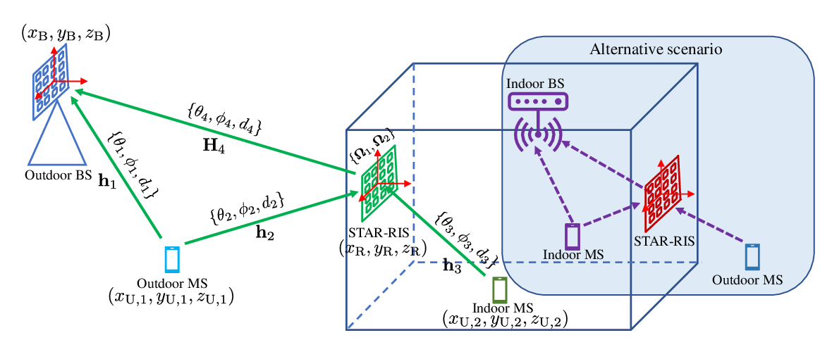
The STAR-RIS-aided 3D localization system, comprising one multi-antenna BS, one multi-element STAR-RIS, one single-antenna indoor MS, and one single-antenna outdoor MS, is depicted in the unshaded area in Fig. 1. By post-processing the pilot signals received over the uplink, the outdoor BS is capable of localizing the two MSs simultaneously, termed as simultaneous indoor and outdoor localization. Note that the coverage of the proposed system depends on the BS capabilities and the area of influence of the STAR-RIS [17]. Alternatively, an indoor BS can also localize one indoor MS and one outdoor MS with the assistance of one STAR-RIS, as depicted in the shaded region in Fig. 1. In this paper, we focus on the former scenario and leave the latter for future investigations.
In the studied 3D localization system, the BS and STAR-RIS are assumed to be equipped with antennas and passive scattering elements, respectively. Without loss of generality, we further assume that both the BS and STAR-RIS employ the uniform planar array (UPA) structure parallel to the plane. They can also be placed parallel to the plane. In this sense, the corresponding array response vectors discussed in Section II-A need to be modified accordingly. Recall that STAR-RIS has two operation functionalities, i.e., reflection and refraction, which can be realized simultaneously via two separate series of phase shifters. Therefore, the operation of STAR-RIS can be represented by two independent control matrices, one for controlling reflection and the other for controlling refraction.
II-A Channel Model
The system adopts millimeter wave frequency band for its operation thanks to the availability of substantial spectrum. Thus, we consider the Saleh-Valenzuela parametric channel model to construct all the four individual channels, marked by the solid arrows in Fig. 1. The direct line-of-sight (LoS) channel between the outdoor MS and the -antenna outdoor BS is denoted as and is mathematically expressed as follows:
| (1) |
where (in meters) and (for the sake of simplicity, we assume that ) are the distance and path loss between the outdoor MS and the outdoor BS, respectively, is the wavelength of the carrier frequency, and and are the azimuth and elevation AoAs associated with , respectively. In the literature, we can also consider the free-space path loss, modeled as , where (in KHz) is the carrier frequency, defined as with being the speed of light. In addition, the standard 3GPP urban micro (UMi) path loss model can be considered, according to which holds: , where needs to be included in GHz [18].
As the BS’s antenna array is parallel to plane, the array response vectors and can be written as [19]:
| (2) | ||||
| (3) |
where with and being the number of horizontal and vertical BS antennas, respectively, and and denote their inter-element spacing in the horizontal and vertical axes, which are set as half-wavelength without loss of generality. Similarly, the other two channels linking the two MSs and the STAR-RIS, e.g., and , can be presented in the same manner, as:
| (4) |
for and , where is the number of STAR-RIS elements with and denoting the numbers in the horizontal and vertical axes, respectively. Note that the array response vectors and in (4) possess the same format compared to those in (1) but may differ in dimension if and . Finally, and follow the same assumption as that made for .
The channel between the STAR-RIS and BS, i.e., , is expressed as follows:
| (5) |
provided that the BS and the STAR-RIS are deployed in parallel without any biased orientation in terms of their antenna (element) arrays. As seen from Fig. 1, there does not exist a direct LoS path between the outdoor BS and the indoor MS due to the blockage incurred by the wall in between them. The only path connecting them is the refraction route via the STAR-RIS. Unlike the indoor MS, there exist one direct LoS path and one reflection path via the STAR-RIS between the outdoor MS and the outdoor BS.
In the channel model, we consider only LoS paths for all the individual channels; the extension for the multipath scenario are only examined in the numerical study in Section V by adding random errors. We ignore the possible orientations between the two UPAs (one for BS and the other for STAR-RIS), since they can be known in priori and compensated when implementing practical estimation algorithms for the angular parameters, i.e., azimuth and elevation AoAs.
II-B Geometric Relationship
Given a pair of nodes, the geometric relationship is built between their Cartesian coordinates and the latent channel parameters, e.g., , , and in (1). The Cartesian coordinates of the BS and STAR-RIS as well as the outdoor and indoor MSs are , , , and , respectively. The relationship between the distances and a pair of Cartesian coordinates are listed below:
| (6) | ||||
| (7) | ||||
| (8) |
By introducing the three-element vector for , the geometric relationship between the angular parameters and the Cartesian coordinates of the nodes can be expressed as
| (9) | ||||
| (10) | ||||
| (11) |
II-C Signal Model
It is known that the STAR-RIS has two operation functionalities, i.e., reflection and refraction, which are realized by two separate series of phase shifters. We introduce two phase control matrices, i.e., for controlling refraction and for controlling reflection, which are diagonal matrices with each diagonal element satisfying the unit-modulus constraints, e.g., , . However, non-ideal reflection and refraction bring attenuation loss, results in reduced modulus, i.e., and [20]. We consider the 3D localization via the uplink transmission, where the two users send their SRSs towards the BS in a NOMA manner. The received signal during the th time slot, for , can be mathematically expressed as
| (12) |
where is the SRS from the outdoor MS, is the SRS from the indoor MS, and coefficients (for refraction) and (for reflection) are used to control the power splitting for the two different operational modes of the STAR-RIS, normalized as . The received signal at the BS is further corrupted by the white Gaussian noise , and each element of follows complex Gaussian distribution with zero mean and variance. During the th time slot, the refraction matrix and the reflection matrix are considered at the STAR-RIS. In order to ensure good estimates of the channel parameters and the locations of the MSs, and vary from one time slot to another, i.e., and . The design of the refractive/reflective beam sweeping will be optimized in Section III-C and verified through our numerical results in Section V.
The received signal vector in (12) can be further expressed as
| (13) |
where and , . By stacking all ’s column by column, we get the expression:
| (14) |
where denotes the -element all-one vector, , , , and with . Without loss of generality, we assume that the sum transmit power constraint is applied for each time slot, i.e., , , and introduce coefficients and for characterizing the power allocation between the two MSs, satisfying , , and . Based on the received signals across time slots, the BS estimates the Cartesian coordinates of both the indoor and outdoor users, enabling 3D localization.
Applying vectorization to in (II-C), we get the following expression:
| (15) |
where and . The expression in (II-C) can be re-written as:
| (16) |
by introducing the following three new notations:
| (17) | ||||
| (18) | ||||
| (19) |
As we can see from (17) to (19), is independent of the STAR-RIS design, while and are functions of and , respectively.
Upon the STAR-RIS deployment, we assume that the BS knows the exact/precise location of the STAR-RIS. Thus, we assume that the BS has exact information on in terms of the parameters , , and . Thus, , , and in (16) are known measurement matrices to the BS (the BS also knows the refractive/reflective phase configurations due to its interaction with the STAR-RIS controller) in the theoretical performance limit analyses in Section III and localization algorithm development in Section IV. However, this assumption will be relaxed and its effect will be examined in Section V since perfect information on is usually infeasible in practice.
III Cramér Rao Lower Bound Analyses
In this section, we summarize the CRLBs on the estimation of the intermediate channel parameters from [10], followed by the 3D Cartesian coordinates’ estimation. This two-step approach can be commonly seen in the literature [7, 8, 21]. We also present the refraction/reflection optimization of the STAR-RIS for the 3D localization objective, where the case is considered and its optimal solution is found. 11 1 In general, a reasonable training overhead is required in order to achieve satisfactory localization performance for both users. Thus, in this work, we only focus on the scenario with slightly larger than , which fits well with the aforementioned statement. As said, we can find the optimal STAR-RIS design for such a case, detailed in Section III-C.
III-A Estimation of Channel Parameters
The unknown channel parameters to be estimated are those included in , , and , i.e., the nine-tuple . Since the additive noise follows complex Gaussian distributed, by introducing from (16), the Fisher information matrix for is obtained as:
| (20) |
The information on the partial derivatives in (20) related to parameters in , , and can be referred to [10] for more details.
For any unbiased estimator (denoted by ) for the channel parameters, we can calculate the CRLB on the error covariance matrix as follows:
| (21) |
where the notation for square matrices and means for any valid vector . The expression (21) indicates that the estimation error variance for each individual channel parameter in is lower bounded by the corresponding diagonal element in , which indicates the best performance any unbiased estimator can reach in theory.
III-B Estimation of 3D Cartesian Coordinates
Our ultimate goal is to estimate the 3D Cartesian coordinates of the indoor and outdoor MSs. Therefore, after estimating the channel parameters, we need to map them to 3D Cartesian coordinates, e.g., , based on the geometrical relationship among the BS, the STAR-RIS, and the two MSs, discussed in Section II-B. For the CRLB evaluation of , we resort to the Jacobian matrix , which links the connection between the channel parameters and the 3D Cartesian coordinates of the two MSs . Each th element of is expressed as:
| (22) |
Again, we omit the details on the calculation of each individual derivative in (22), which can be found in [10].
In addition, it can be easily seen that only the channel parameters are related to the coordinates of the outdoor MS, and only the parameters are related to the coordinates of the indoor MS, as concluded from (10) and (11). Therefore, the Jacobian matrix has the following form:
| (23) |
where the submatrix consists of the partial derivatives related to the outdoor MS, and the submatrix consists of the partial derivatives related to the indoor MS.
The Fisher information of can be then expressed as [8]
| (24) |
Similar to (21), we have the inequality for the CLRB:
| (25) |
The performance lower bounds on the root mean square error (RMSE) of the position estimation of the outdoor and indoor MSs are:
| (26) | ||||
| (27) |
where and are the unbiased estimates of and , respectively.
III-C Localization-Optimal Design for the STAR-RIS
In this subsection, we consider the optimization of STAR-RIS during the pilot transmission, aiming at maximizing the overall 3D localization performance of the two MSs. The scenario with is considered, where we aim at optimizing the STAR-RIS based on the inverse matrix of the Fisher information matrix. By introducing , , , and , the expression of in (21) can be expressed as [22, 23]
| (28) |
where is the orthogonal projection onto the column space of for and .
In order to simplify the diagonal terms in (28), we rewrite and as and , where , , and contain the remaining terms of (excluding , , and ), respectively. Our goal is to optimize in and in in order to obtain the best theoretical localization performance. By further dividing into two submatrices, i.e., as , we can derive the expressions and . For the sake of tractability for the STAR-RIS optimization (i.e., and ), we maximize the principal angle (within ) between the subspaces of and by following [22], which is equivalent to minimizing , i.e.,
| (29) |
We focus on in the first term and in the second term of (29), which are detailed as
| (30) | ||||
| (31) |
by using the following properties: , , , and for matrices , , , and meeting the dimension requirements.
When training overhead , we can easily find the optimal solution for and that minimize the Frobenius norm in (29), e.g., and with being the transpose of a discrete Fourier transform (DFT) matrix or Hadamard matrix (only for certain integer values). By following this, we have in (30) and in (31), which in turn yields (i.e., we get the largest principal angle between the subspaces of and , which is [24]).
IV Localization Algorithm Development
By aligning with the theoretical analyses studied in Section III, we develop a two-step localization algorithm to estimate the location of the two MSs. In the first step, based on (16) one estimates the channel parameters in , , and . In the second step, by following the geometric relationship in Section II-B, we map the estimates of channel parameters to the coordinates of the MSs. Special attention needs to be paid to the first step for the co-channel interference mitigation/cancellation, i.e., null the other two when estimating one channel. Also, for the channel parameter estimation, we resort to off-grid CS ANM for recovering the sparsity-one channel vectors and root multiple signal classification (root-MUSIC) for extracting the corresponding angular channel parameters, followed by distance estimates using the least squares (LS) principle [25]. For the location mapping of the outdoor MS, we adopt a weighted sum criterion based on the two distance estimates associated with and .
IV-A Co-Channel Interference Cancellation
As an essential process for channel parameter estimation, we need to null the interference for each MS in (16). By multiplying the interference nulling matrix to , for , we get the following
| (32) |
where , , and . We rely on (32) in the next subsection for channel parameter estimation. The co-channel interference can be completely cancelled in (32) in certain situations depending on the relationship among the vector spaces spanned by the column vectors of , , and , respectively [26]. Otherwise, we merge the residual interference to the additive noise term . One way to design is to perform singular value decomposition (SVD) on the combined matrix and take the left singular vectors corresponding to zero singular values [26]. A similar approach can be applied for constructing and .
IV-B Channel Parameter Estimation
All the channel vectors in (16) are in the form of Kronecker product of two array response vectors. It can be seen as sparsity-one signal (i.e., a linear combination of one atom having the same structure as the channel component in the form of Kronecker product of two array response vectors), which is an extreme case under the framework of CS. Therefore, we follow the off-grid CS techniques, i.e., ANM, for recovering the sparsity-one channel vector. This technique has been used in the literature [27, 25] for channel estimation and localization purposes. We first introduce the atomic set [28, 29, 27], as
| (33) |
where each atom possesses the same structure with the linear term in , for . For any vector of the form with each being a coefficient, , and , its atomic norm with respect to the atomic set is written as follows:
| (34) |
where set with being a -way tensor and is a -level block Toeplitz matrix, which results from the Vandermonde decomposition lemma for positive semidefinite Toeplitz matrices [29]. The value for depends on the dimension of , i.e., for , and , for .
The ANM based channel estimation can be formulated as a regularized optimization problem:
| (35) |
where is the regularization term of the atomic norm penalty, and is the estimate of . This problem can be efficiently solved using the Matlab CVX toolbox.
Based on the , the elevation and azimuth AoAs can be extracted by following root-MUSIC algorithm [25] and the distance can be estimated by following LS principle, as
| (36) |
where is the estimate of .
IV-C Location Mapping
Based on the estimate of in (IV-B), we can further resort to root-MUSIC for extracting the angular parameters, denoted by and [25]. Together with the estimate of in (36), the location of the MSs can be calculated by following the geometric relationship in Section II-B.
Specifically, for the location estimate of the outdoor MS, since both and contribute to it, we apply weighted sum principle, as
| (37) |
where the weight is set in a heuristic way by following that the weight is reversely proportional to the path loss.
V Numerical Results
In this section’s numerical investigation, we set the system parameters as follows: , , , and . The numbers of BS antennas, STAR-RIS elements, and SRSs from each MS are set as , , and . The signal-to-noise ratio (SNR) is defined as . The parameter setup is summarized in Table I.
| Parameter | Value | Parameter | Value |
|---|---|---|---|
V-A Effect of Training Overhead
As shown in Section III-C, we find the optimal design of the STAR-RIS for the training overhead . We pick up two values meeting this requirement and compare their impact on the localization performance. The simulation results, including both theoretical and practical, are shown in Fig. 2 for the training overhead , where . In the legend, “ANM” denotes the proposed ANM based 3D localization scheme while “Theo” stands for the theoretical performance limit analyses. From the theoretical ones characterized by CRLBs, we know that higher training overhead can bring better localization performance, up to centimeter level for both MSs. Moreover, the indoor MS can achieve better performance than the outdoor MS in such a unbalanced setup on and since the STAR-RIS power splitting coefficient is large (Namely, more percent of energy is refracted towards the BS via the STAR-RIS). The practical results from ANM are consistent with the theoretical studies. The performance gain brought by increasing the training overhead from to is not so obvious from the practical results, especially in the low SNR regime. However, a constant gain (roughly dB) is observed from the theoretical CRLB results across all the SNR values for both users.

V-B Effect of Power Splitting and Allocation
The performance of 3D localization is not only affected by the training overhead but also the two parameters, i.e., for controlling power splitting at STAR-RIS and for controlling power allocation between the two users. For the training overhead , the simulation results with different setups on and are shown in Fig. 3. As we can see that when a balanced setup is adopted, i.e., , the performance gap between the two MSs’ position estimation is small. However, in the other setup, i.e., , the gap is obvious. By carefully choosing the values for the two parameters, we can simultaneously achieve the QoS requirements for both users.

V-C Effect of STAR-RIS Design
In this subsection, we evaluate the effect of the STAR-RIS design (under the condition of training overhead ) by considering two different cases: i) and are designed according Section III-C; ii) the phases of and are randomly generated. The simulation results are shown in Fig. 4. As expected, the first case outperforms the second one, since according to Section III-C it is optimal. The performance gain between the two cases is obvious with different setups for and . For instance, when and , more than dB gain in terms of SNR can be obtained for the indoor MS by following the optimal STAR-RIS design compared to the random phase design.

V-D Effect of Imperfect STAR-RIS-to-BS Channel
In this section, we examine the effect of imperfectness of the STAR-RIS-to-BS channel on the 3D localization performance. Different from the previous subsections, here, we assume that the STAR-RIS-to-BS channel matrix is available but in the form of imperfectness during the localization process. We introduce individual random variation to each of the channel parameters in the STAR-RIS-to-BS channel, e.g., , , . Such variations can be introduced by practical algorithms for estimating them. We further assume that the variations follow uniform distribution, i.e., , . The values of and jointly determine the level of imperfectness of the STAR-RIS-to-BS channel. In this experiment, we evaluate two cases: i) in meter and in radian, ii) in meter and in radian, under training overhead . The simulation results are provided in Fig. 5, where and . As expected, the localization performance degrades when and increases, especially in the high SNR regime.

V-E Effect of MPCs
The proposed localization algorithm purely relies channel parameters associated with the LoS path. Therefore, the strength of the non-line-of-sight (NLoS) path will negatively affect the localization performance. In principle, the stronger the strength, the worse the localization performance. In this subsection, we pick up different setups on the average sum power of the NLoS paths (revealed by the distance) and evaluate accordingly their negative effect on the localization performance. We introduce two MPCs to , , and while keeping perfect LoS condition for . The introduced MPCs for , for , comprise the following channel parameters: case i) and and case ii) and . The simulation results are shown in Fig. 6, where we observe that the stronger the MPCs, the worse the localization performance. Even though there are works on leveraging NLoS paths for enhancing localization performance [30, 31], we will leave such an extension for our future investigation.

VI Conclusion and Future Work
In this paper, we studied the fundamental 3D localization performance limits of STAR-RIS-empowered millimeter wave MIMO systems for simultaneously serving one indoor and one outdoor MSs. We presented a practical localization algorithm based on ANM, which approaches the theoretical performance limits characterized by our derived CRLBs. In addition, we thoroughly investigated the effect of training overhead, energy splitting at the STAR-RIS, the power allocation between the two MSs, the STAR-RIS design, the imperfectness of STAR-RIS-to-BS channel, as well as the role of the presence of MPCs on the localization performance of the two MSs, offering some useful insights for future practical implementations. In future works, we will extend the theoretical CRLB analyses to general multipath scenarios and exploit the availability of MPCs for further enhancing the localization performance of the two MSs in the design of practical localization algorithms.
References
- [1] C. Huang, A. Zappone, G. C. Alexandropoulos, M. Debbah, and C. Yuen, “Reconfigurable intelligent surfaces for energy efficiency in wireless communication,” IEEE Trans. Wireless Commun., vol. 18, no. 8, pp. 4157–4170, Aug. 2019.
- [2] M. Di Renzo et al., “Smart radio environments empowered by reconfigurable AI meta-surfaces: an idea whose time has come,” EURASIP J. Wireless Comm. and Networking, vol. 2019, p. 129, 2019.
- [3] G. C. Alexandropoulos, G. Lerosey, M. Debbah, and M. Fink, “Reconfigurable intelligent surfaces and metamaterials: The potential of wave propagation control for 6G wireless communications,” IEEE ComSoc TCCN Newslett., vol. 6, no. 1, pp. 25–37, Jun. 2020.
- [4] Q. Wu, S. Zhang, B. Zheng, C. You, and R. Zhang, “Intelligent reflecting surface aided wireless communications: A tutorial,” IEEE Trans. Commun., vol. 69, no. 5, pp. 3313–3351, May 2021.
- [5] E. Calvanese Strinati, G. C. Alexandropoulos, H. Wymeersch, B. Denis, V. Sciancalepore, R. D’Errico, A. Clemente, D.-T. Phan-Huy, E. D. Carvalho, and P. Popovski, “Reconfigurable, intelligent, and sustainable wireless environments for 6G smart connectivity,” IEEE Commun. Mag., vol. 59, no. 10, pp. 99–105, Oct. 2021.
- [6] H. Wymeersch, J. He, B. Denis, A. Clemente, and M. Juntti, “Radio localization and mapping with reconfigurable intelligent surfaces: Challenges, opportunities, and research directions,” IEEE Veh. Technol. Mag., vol. 15, no. 4, pp. 52–61, Dec. 2020.
- [7] J. He, H. Wymeersch, L. Kong, O. Silvén, and M. Juntti, “Large intelligent surface for positioning in millimeter wave MIMO systems,” in Proc. IEEE VTC-Spring, 2020, pp. 1–5.
- [8] A. Elzanaty, A. Guerra, F. Guidi, and M.-S. Alouini, “Reconfigurable intelligent surfaces for localization: Position and orientation error bounds,” IEEE Trans. Signal Process., vol. 69, Aug. 2021.
- [9] G. C. Alexandropoulos, I. Vinieratou, and H. Wymeersch, “Localization via multiple reconfigurable intelligent surfaces equipped with single receive RF chains,” IEEE Wireless Commun. Lett., vol. 11, no. 5, pp. 1072–1076, 2022.
- [10] J. He, A. Fakhreddine, and G. C. Alexandropoulos, “Simultaneous indoor and outdoor 3D localization with STAR-RIS-assisted millimeter wave systems,” in proc. IEEE Vehicular Technology Conference (Fall), September, 2022, pp. 1–6.
- [11] M. Jian, G. C. Alexandropoulos, E. Basar, C. Huang, R. Liu, Y. Liu, and C. Yuen, “Reconfigurable intelligent surfaces for wireless communications: Overview of hardware designs, channel models, and estimation techniques,” Int. Conv. Netw., vol. 3, no. 1, pp. 1–32, Mar. 2022.
- [12] G. C. Alexandropoulos, N. Shlezinger, and P. del Hougne, “Reconfigurable intelligent surfaces for rich scattering wireless communications: Recent experiments, challenges, and opportunities,” IEEE Commun. Mag., vol. 59, no. 6, pp. 28–34, Jun. 2021.
- [13] G. C. Alexandropoulos, N. Shlezinger, I. Alamzadeh, M. F. Imani, H. Zhang, and Y. C. Eldar, “Hybrid reconfigurable intelligent metasurfaces: Enabling simultaneous tunable reflections and sensing for 6G wireless communications,” 2021. [Online]. Available: https://arxiv.org/pdf/2104.04690
- [14] Y. Liu, X. Mu, J. Xu, R. Schober, Y. Hao, H. V. Poor, and L. Hanzo, “STAR: Simultaneous transmission and reflection for 360∘ coverage by intelligent surfaces,” IEEE Wireless Commun., vol. 28, no. 6, pp. 102–109, Dec. 2021.
- [15] C. Wu, C. You, Y. Liu, X. Gu, and Y. Cai, “Channel estimation for star-ris-aided wireless communication,” IEEE Commun. Lett., vol. 26, no. 3, pp. 652–656, 2022.
- [16] X. Yue, J. Xie, Y. Liu, Z. Han, R. Liu, and Z. Ding, “Simultaneously transmitting and reflecting reconfigurable intelligent surface assisted noma networks,” IEEE Trans. Wireless Commun., pp. 1–1, 2022.
- [17] G. C. Alexandropoulos, M. Crozzoli, D.-T. Phan-Huy, K. D. Katsanos, H. Wymeersch, P. Popovski, P. Ratajczak, Y. Bénédic, M.-H. Hamon, S. Herraiz Gonzalez, R. D’Errico, and E. Calvanese Strinati, “Smart wireless environments enabled by riss: Deployment scenarios and two key challenges,” in Proc. Joint European Conference on Networks and Communications & 6G Summit, Grenoble, France, Jun. 2022, pp. 1–6.
- [18] M. R. Akdeniz, Y. Liu, M. K. Samimi, S. Sun, S. Rangan, T. S. Rappaport, and E. Erkip, “Millimeter wave channel modeling and cellular capacity evaluation,” IEEE J. Sel. Areas Commun., vol. 32, no. 6, pp. 1164–1179, Jun. 2014.
- [19] Y. Tsai, L. Zheng, and X. Wang, “Millimeter-wave beamformed full-dimensional MIMO channel estimation based on atomic norm minimization,” IEEE Trans. Commun., vol. 66, no. 12, pp. 6150–6163, Dec. 2018.
- [20] Q. Wu and R. Zhang, “Beamforming optimization for wireless network aided by intelligent reflecting surface with discrete phase shifts,” IEEE Trans. Commun., pp. 1–1, 2019.
- [21] A. Shahmansoori, G. E. Garcia, G. Destino, G. Seco-Granados, and H. Wymeersch, “Position and orientation estimation through millimeter-wave MIMO in 5G systems,” IEEE Trans. Wireless Commun., vol. 17, no. 3, pp. 1822–1835, 2018.
- [22] L. L. Scharf and L. T. McWhorter, “Geometry of the Cramer-Rao bound,” Signal Process., vol. 31, no. 3, pp. 301–311, Apr. 1993.
- [23] P. Pakrooh, A. Pezeshki, L. L. Scharf, D. Cochran, and S. D. Howard, “Analysis of Fisher information and the Cramér–Rao bound for nonlinear parameter estimation after random compression,” IEEE Trans. Signal Process., vol. 63, no. 23, pp. 6423–6428, Dec. 2015.
- [24] G. H. Golub and C. F. Van Loan, Matrix computations. JHU press, 2013.
- [25] J. He, A. Fakhreddine, C. Vanwynsberghe, H. Wymeersch, and G. C. Alexandropoulos, “3D localization with a single partially-connected receiving RIS: Positioning error analysis and algorithmic design,” arXiv preprint arXiv:2212.02088, 2022.
- [26] H. Sung, S.-H. Park, K.-J. Lee, and I. Lee, “Linear precoder designs for k-user interference channels,” IEEE Trans. Wireless Commun., vol. 9, no. 1, pp. 291–301, 2010.
- [27] J. He, H. Wymeersch, and M. Juntti, “Channel estimation for RIS-aided mmWave MIMO systems via atomic norm minimization,” IEEE Trans. Wireless Commun., pp. 1–1, 2021.
- [28] Z. Yang and L. Xie, “Exact joint sparse frequency recovery via optimization methods,” IEEE Trans. Signal Process., vol. 64, no. 19, pp. 5145–5157, Oct 2016.
- [29] G. Tang, B. N. Bhaskar, P. Shah, and B. Recht, “Compressed sensing off the grid,” IEEE Trans. Inf. Theory, vol. 59, no. 11, pp. 7465–7490, 2013.
- [30] K. Witrisal, P. Meissner, E. Leitinger, Y. Shen, C. Gustafson, F. Tufvesson, K. Haneda, D. Dardari, A. F. Molisch, A. Conti, and M. Z. Win, “High-accuracy localization for assisted living: 5G systems will turn multipath channels from foe to friend,” IEEE Signal Process. Mag., vol. 33, no. 2, pp. 59–70, 2016.
- [31] R. Mendrzik, H. Wymeersch, G. Bauch, and Z. Abu-Shaban, “Harnessing NLOS components for position and orientation estimation in 5G millimeter wave MIMO,” IEEE Trans. Wireless Commun., vol. 18, no. 1, pp. 93–107, 2019.