PAMI: partition input and aggregate outputs for model interpretation

Wei Shi Affiliation: Sun Yat-sen University Email: shiw58@mail2.sysu.edu.cn Wentao Zhang Affiliation: Sun Yat-sen University Email: zhangwt65@mail2.sysu.edu.cn Weishi Zheng Affiliation: Sun Yat-sen University Email: wszheng@ieee.org Ruixuan Wang Affiliation: Sun Yat-sen University Email: wangruix5@mail.sysu.edu.cn

Abstract

There is an increasing demand for interpretation of model predictions especially in high-risk applications. Various visualization approaches have been proposed to estimate the part of input which is relevant to a specific model prediction. However, most approaches require model structure and parameter details in order to obtain the visualization results, and in general much effort is required to adapt each approach to multiple types of tasks particularly when model backbone and input format change over tasks. In this study, a simple yet effective visualization framework called PAMI is proposed based on the observation that deep learning models often aggregate features from local regions for model predictions. The basic idea is to mask majority of the input and use the corresponding model output as the relative contribution of the preserved input part to the original model prediction. For each input, since only a set of model outputs are collected and aggregated, PAMI does not require any model details and can be applied to various prediction tasks with different model backbones and input formats. Extensive experiments on multiple tasks confirm the proposed method performs better than existing visualization approaches in more precisely finding class-specific input regions, and when applied to different model backbones and input formats. The source code will be released publicly.

1 Introduction

Deep learning models have shown human-level performance in various machine learning tasks and started to be applied in real scenarios, such as face identification he2018wasserstein; yan2019vargfacenet; kim2020groupface, medical image analysis chen2019med3d; li2021medical; sanderson2022fcn, and language translation wu2021r; xu2021bert; takase2021rethinking. However, current deep learning models often lack interpretations for their decision making, which hinders the massive deployment of intelligent systems particularly in high-risk applications like medical diagnosis and autonomous driving.

To improve interpretation of model predictions, multiple visualization approaches have been proposed to localize input regions or components which are more relevant to the model prediction given any specific input to the model. For image classification task as an example, the class activation map (CAM) and its variants utilize the output (i.e., feature maps) of certain convolutional layer in the convolutional neural networks (CNNs) and their contribution weights to find the image regions which are responsible for the specific model prediction given any input image zhou2016learning; selvaraju2017grad; chattopadhay2018grad; wang2020score; liu2022partial, and the back-propagation approaches propagate the CNN output layer-by-layer to the input image space either based on gradient information (or its modified versions) at each layer springenberg2015striving; selvaraju2017grad; chattopadhay2018grad; srinivas2019full; sundararajan2017axiomatic or based on the relevance between input elements and output at each layer binder2016layer; bach2015pixel; montavon2017explaining; iwana2019explaining. While the CAM-like approaches can only roughly localize relevant regions due to the lower resolution of feature maps, the back-propagation approaches often just find sparse and incomplete object regions relevant to the model prediction. Moreover, both types of approaches need either part of or the whole model structure and parameter details, which may be unavailable in some applications due to privacy or security concerns. When the model details are not available, the occlusion method may be utilized to roughly localize image regions relevant to the model prediction by occluding each local patch and checking the change in model output zeiler2014visualizing; petsiuk2018rise. However, the occlusion method often only localizes the most discriminative object part and misses the other parts which actually also contribute to the model prediction. LIME ribeiro2016should is another method without requiring model details for model interpretation by locally approximating the model decision surface for any specific input, but it can often estimate the contributions of a subset of input parts and require an optimization process for interpretation of a specific model prediction. Furthermore, most existing visualization approaches for interpretation of model predictions are developed for specific type of tasks (e.g., just for image classification), model backbone (e.g., for CNNs), and input format (e.g., just for image data). Substantial efforts are often required to adapt one visualization approach to various tasks (e.g., image caption) with different model backbones (e.g., Transformer backbone) or input formats (e.g., sequence of items).

Different from existing visualization approaches, a simple yet effective visualization framework for interpretation of model predictions is proposed in this study. The proposed framework, called PAMI (‘Partition input and Aggregate outputs for Model Interpretation’), is inspired by the observation that both humans and popular deep learning models extract and aggregate features of local regions for image understanding and decision making. Suppose a well-trained image classifier predicts an input image as a specific class. To find the relevant image regions and their contributions to the model prediction, the proposed framework first partitions the input into multiple parts, and then feeds only one part (with the remaining regions masked) to the model to obtain the corresponding output probability of the specific class. Aggregating the output probabilities over all the individual parts would result in an importance map representing the contribution of each input part to the original model prediction. In contrast to existing visualization approaches, the proposed PAMI framework does not require model structure and parameter details, can more likely find all possible input parts which are relevant to the model prediction, more precisely localize relevant parts, and work for various model backbones with different input formats. Such merits of the proposed PAMI framework has been confirmed by extensive experiments on multiple tasks with different model backbones and input formats.

2 Related Work

In computer vision, post-hoc interpretation of deep learning models focuses on either understanding of model neurons (e.g., convlutional kernels, output elements) which is independent of input information erhan2009visualizing; mahendran2015understanding; jason2015understanding; kim2018interpretability; bau2020understanding, or understanding of a specific model prediction given an input image lim2021building; petsiuk2018rise; elliott2021explaining; selvaraju2017grad; chattopadhay2018grad. This study belongs to the latter one, i.e., trying to understand what information in the input causes the specific model prediction.

Multiple approaches have been proposed for understanding of model predictions, including the activation map approach chattopadhay2018grad; selvaraju2017grad; zhou2016learning; jiang2021layercam, the back-propagation approach iwana2019explaining; zeiler2014visualizing; gu2018understanding; zeiler2014visualizing, the perturbation approach petsiuk2018rise; fong2017interpretable, the local approximation approach ribeiro2016should; zhou2015object and the optimization-based approach lim2021building; elliott2021explaining. The activation map approach often obtains a class-specific activation map with the weighted sum of all feature maps often at the last convolutional layer, and considers the regions with stronger activation relevant to the specific model output chattopadhay2018grad; selvaraju2017grad; wang2020score; zhou2016learning. Since the activation map is often much smaller than the input image, only approximate image regions corresponding to the stronger activation regions can be localized for interpretation of the specific model prediction. Different from the activation approach which often works at higher layer of the deep learning model, the back-propagation approach tries to estimate the importance of each input pixel by propagating the specific model output layer-by-layer back to the input space. This can be obtained by calculating the gradient of the specific model output with respect to input elements at each layer springenberg2015striving; selvaraju2017grad; chattopadhay2018grad; srinivas2019full; sundararajan2017axiomatic, the input-relevant contribution of each kernel at each layer kindermans2018learning, or the relevance between output and each input element at each layer binder2016layer; bach2015pixel; montavon2017explaining; iwana2019explaining. The back-propagation approach considers each input pixel as an independent component and often only a subset of disconnected pixels in the relevant regions are estimated to be relevant to the model prediction.

To find local image regions rather than disconnected pixels relevant to the model prediction, the perturbation approach has been proposed by perturbing local image regions somehow and checking the change in model output of the predicted class fong2017interpretable; zeiler2014visualizing. If certain perturbed local region causes large drop in the output, the local region in the input image is considered crucial to the original model prediction. Perturbation can be in the form of simply masking a local region by a constant pixel intensity zeiler2014visualizing, by neighboring image patches zintgraf2017visualizing, or by blurring the original region information with a constant value or smoothing operator petsiuk2018rise; fong2017interpretable. This approach often can find only the most discriminative part of the relevant regions which are responsible for the model prediction, because perturbing less-discriminative part of the relevant regions often does not cause much drop in model output. Besides the perturbation approach, the local approximation approach provides another way to estimate the contribution of each meaningful image region (e.g., object parts, background region) to the model prediction ribeiro2016should; wang2020score; fong2017interpretable. This approach assumes that the model decision surface is locally linear in the region-based feature space for any specific input, and therefore can be approximated with a linear model in the feature space. The weight parameters in the linear model can directly indicate the contribution of each meaningful image region to the original model output, thus obtaining image regions most relevant to the model prediction.

While most of these visualization approaches to interpretation of model predictions were originally developed for image classification models, they have been extended or modified for other tasks danilevsky2020survey; wallace2020interpreting or other deep learning models chefer2021transformer; li2019graph. Besides these approaches, prototype-based nauta2021neural; rymarczyk2021protopshare and and attention-based obeso2022visual approaches have also been proposed for model interpretation. Note that except the local approximation approach and part of the perturbation approach (e.g., the occlusion method fong2017interpretable, most approaches require at least part of the model structure and parameter details in order to find input parts which are relevant to the model prediction.

Refer to caption — Figure 1: The proposed PAMI framework with the sliding window based (left half) or the pre-segmentation based (right half) input partition strategy. Each time only one local part of the input is preserved and the remaining parts are masked (blurred here).

3 Method

In this study, we aim to provide interpretation for model prediction given any specific input to a well-trained and fixed deep learning model. The interpretation is demonstrated by estimating relative contribution of each input part to the specific model prediction and correspondingly localizing input regions or elements which are relevant to the model prediction. It is worth noting that no model structure and parameter details are assumed to be known during the model interpretation process.

3.1 Motivation

Although humans can often instantly recognize objects in images, certain attention mechanism in human brain is likely involved in the process of object recognition itti2001computational; petersen2012attention. In other words, humans often need to implicitly or explicitly attend to local regions for image understanding and object recognition. While the detailed human attention mechanism is yet to be further explored, initial studies desimone1995neural suggest that most local parts of an object in an image help humans recognize the object, and appearance of only an individual object part could help humans recall the corresponding class of the object. Consistent with the visual attention studies, recent exploration of convolutional neural networks (CNNs) shows that convolutional kernels even at higher convolutional layers (i.e., closer to the CNN output) often have smaller receptive fields than expected luo2016understanding. Considering that a global pooling is performed at the last convolutional layer in most CNN classifier models, it is widely accepted that CNN models largely depend on the collection of local image region features for image classification. For the other type of deep learning model backbone Transformer and its variants (e.g., ViT dosovitskiy2020image, Swin Transformer liu2021swin), since most items in the input sequence at each model layer correspond to components (e.g., words for a sentence input, image patches for an image input) of the original input, the final model prediction also largely depends on the collection of local features of the original input. With the above observation, we hypothesize that the model output response to each single component of the original input may directly imply the importance of the single input component for the specific model prediction.

3.2 The proposed PAMI framework

The proposed interpretation framework is demonstrated in Figure 1. For image classification task as an example, given a well-trained classifier model $f(\cdot)$ and any input image $\mathbf{x}$ , denote by $f_{c}(\mathbf{x})$ the output prediction probability of the input image belonging to the $c$ -th class. Suppose the model predicts the input as the $k$ -th class, i.e., $f_{k}(\mathbf{x})$ is the maximum over all the output probabilities. To interpret the classifier’s prediction, the proposed framework first partitions the input into multiple either overlapped or non-overlapped parts (see the following subsections), and then with the $j$ -th individual part preserved and all the remaining image regions masked, the output probability $f_{k}(\mathbf{x}_{j})$ of the $k$ -th class for the majority-masked input $\mathbf{x}_{j}$ is used to estimate the relative contribution of the preserved $j$ -th image part to the original model prediction $f_{k}(\mathbf{x})$ . By collecting and aggregating the output responses $f_{k}(\mathbf{x}_{j})$ ’s over all the partitioned image parts, an importance map with the same spatial size as that of the input image $\mathbf{x}$ can be generated to represent the contribution of each input element (i.e., pixel here). Local image regions with correspondingly higher response values in the importance map are supposed to contribute more to the model prediction $f_{k}(\mathbf{x})$ , thus providing visual evidence for the model prediction. It is worth noting that the interpretation framework can be applied to different tasks (e.g., image caption and sentiment analysis) with various input formats.

3.2.1 Input partition strategy I: sliding window

One simple way to partition input is to apply the sliding window strategy with a pre-defined window size and sliding step size, where the window is in certain regular shape (e.g., circular or rectangular). In this way, the original input can be easily partitioned into multiple parts, and each part can be more or less overlapped by its neighboring parts determined by window size and sliding step size. For each partitioned part, all the remaining image regions will be masked somehow (e.g., by black pixels or blurred version of the original regions), and the output probability of the originally predicted class can be directly obtained with the majority-masked image as input. Since each input element (e.g., pixel of an input image) could be covered by multiple partitioned parts, the contribution of each input element in the final importance map can be obtained by averaging the output probabilities of the originally predicted class over all the partitioned parts covering the input element.

Note that the window size would affect the resolution level of the final importance map. Although smaller window would result in desired higher resolution, an image part with much smaller size (i.e., too small window) could contain little semantic information such that it becomes challenging for the framework to estimate the contribution of the smaller image part to a specific model prediction. In practice, users can choose one appropriate window size for interpretation of model prediction, or multiple window sizes for interpretation at multiple scales of image parts.

3.2.2 Input partition strategy II: pre-segmentation

Another way to partition input is to pre-segment the input into multiple parts with certain segmentation strategy. When the input is an image, various unsupervised segmentation algorithms can be adopted for pre-segmentation of the input. In this study, super-pixel segmentation algorithms are used for input image partition felzenszwalb2004efficient; ren2003learning; meyer1992color; bergh2012seeds. With a particular super-pixel segmentation method, an input image can be partitioned into multiple non-overlapped parts (i.e., super-pixels), with each part often having irregular form of region boundary and likely containing homogeneous visual information. As introduced above, the contribution of each super-pixel to the model prediction can be obtained by preserving the single super-pixel and masking the other super-pixels as the input and collecting the model output response of the predicted class to the majority-masked input.

In practice, due to the imperfect performance of any single super-pixel segmentation method, some super-pixels may contain parts of both object region and background region, resulting in the importance map where part of background regions also have relatively higher responses. To alleviate such an issue, multiple super-pixel segmentation methods are employed, and multiple importance maps based on these segmentation methods are then averaged to estimate the contribution of each input element (e.g., pixels) to the original model prediction. The average importance map may be further improved by running the above process once more (i.e., second run), in which the super-pixel segmentation methods are performed on the average importance map rather than the original input image. In addition, when generating each majority-masked input, the highly smoothed version of the original input image is used to fill the corresponding masked regions.

Compared to the sliding window strategy, the partitioned parts by the pre-segmentation strategy have more precise and reasonable region boundaries particularly for image data. This in turn often leads to the final importance map with clear boundaries between object regions and background regions, thus more precisely locating the image regions which contribute to the model prediction. Note that both input partition strategies also work when input is a sequence of items. For example, when input is a sentence as in the sentiment analysis task, any input can be partitioned into words or phrases with either the sliding window strategy or appropriate pre-segmentation strategy.

3.3 Comparison with relevant studies

The proposed PAMI framework can provide interpretation of model prediction without requiring to know model structure and parameter information. In contrast, most existing interpretation methods requires either part of or the whole model details. For example, CAM and its variants need the feature maps from certain convolutional layers and part of model parameters in order to obtain the final class activation map zhou2016learning; selvaraju2017grad; chattopadhay2018grad; wang2020score; liu2022partial, and the gradient-based methods need all the model details to calculate gradient information over model layers springenberg2015striving; selvaraju2017grad; chattopadhay2018grad; srinivas2019full; sundararajan2017axiomatic. One exception is the occlusion method zeiler2014visualizing; petsiuk2018rise which does not require model details as the proposed PAMI framework. PAMI can be considered as an opposite version of the occlusion method, i.e., only preserving an input part versus only removing or occluding an input part for estimating the contribution of the input part to the model prediction. In image classification, occluding part of the foreground object in the image may not significantly affect the model prediction because the model can use the other object parts in the image for confident prediction. As a result, occlusion method may neglect contribution of certain object parts to the original model prediction, and often performs worse than the proposed PAMI.

Because the proposed PAMI framework can consider the well-trained model as a black-box, it can potentially work for various backbone structures (e.g., both CNN and Transformer backbones). In contrast, the majority of interpretation methods were proposed for the CNN backbone, and specific modifications are often required when applying existing interpretation methods (e.g., CAM or Grad-CAM) to other backbones like Transformer chefer2021transformer; li2022transcam and graph neural networks pope2019explainability; barcelo2020logical; dehmamy2019understanding. Another merit of the proposed PAMI framework is its potential usage in multiple tasks with different input formats. While this study mainly use the image classification task for evaluation of the PAMI framework, PAMI in principle can be applied to various model prediction tasks, such as image caption and sentiment analysis, where the input data can be in the format of sentence or image. In contrast, most existing interpretation methods do not work across tasks without further modifications or extensions.

The most relevant interpretation methods are RISE petsiuk2018rise and ScoreCAM wang2020score which also estimate the importance map based on linear combination of input masks with weights from model outputs. However, RISE is based on a large set of randomly generated masks and ScoreCAM is based on the feature maps at last convolutional layer of the (CNN) model, both leading to low-resolution and often inappropriate importance maps.

4 Experiments

4.1 Experimental setup

In this study, three image classification datasets ImageNet-2012 ILSVRC15, Pascal VOC 2007 pascal-voc-2007, and COCO 2014 lin2014microsoft were mainly used for evaluation of the proposed PAMI method. In addition, an image caption dataset COCO lin2014microsoft and sentiment analysis dataset Sentiment140 Sentiment140 were also employed to show the wide applications of the proposed method. All the models were from the publicly released resources and evaluated on the corresponding validation or test set (see Table 1 for more details).

Table 1: Models and datasets used in experiments.

Task

Model source

Dataset

Cassification

VGG19bn from PyTorch Paszke_PyTorch_An_Imperative_2019

50000 images of ImageNet-2012 ILSVRC15

validation set with 1000 classes

VGG16 from TorchRay torchray

Ffirst 1000 images of Pascal VOC 2007 pascal-voc-2007

test set with 20 classes

VGG16 from TorchRay torchray

First 1000 images of COCO 2014 lin2014microsoft

instances validation set with 80 classes

Image caption

ClipCap mokady2021clipcap

COCO 2014 lin2014microsoft

Sentiment analysis

Transfomers libary Wolf_Transformers_State-of-the-Art_Natural_2020

Sentiment140 Sentiment140

By default, for the sliding window strategy of the proposed PAMI, circular window with radius 40 pixels and step size 6 pixels was used to generate local image regions. For the pre-segmentation strategy, four super-pixel segmentation algorithms, i.e., felzenszwalb felzenszwalb2004efficient, SLIC ren2003learning, watershed meyer1992color from scikit-image library scikit-image, and SEEDS bergh2012seeds from the OpenCV library opencv_library were utilized respectively for pre-segmentation of each image into multiple regions. Considering region of interest (i.e., relevant region to the model prediction) could vary a lot over images, each segmentation algorithm was run multiple times with different hyper-parameter settings to generate sets of local regions at different scales (see the supplementary A for detailed settings). The importance maps over all hyper-parameter settings and all the four pre-segmentation algorithms were averaged as the estimated importance map. A Gaussian kernel with size $49\times 49$ pixels and standard deviation 100 was used to generate the smoothed (blurred) image for region masking.

The proposed PAMI was compared with widely used visualization methods for interpretation of model predictions, including Gradient simonyan2014deep, GradCAM selvaraju2017grad, ScoreCAM wang2020score, RISE petsiuk2018rise, FullGrad srinivas2019full, MASK fong2017interpretable, Occlusion zeiler2014visualizing, GuidedBP springenberg2015striving, SmoothGrad smilkov2017smoothgrad and LRP montavon2017explaining. The default hyper-parameter setting for each method was adopted (see supplementary B for details). Besides qualitative evaluation, quantitative evaluation was also performed using the pointing game zhang2018top and the insertion metric petsiuk2018rise. In the pointing game, it measures whether the pixel with the highest activation in the importance map is successfully within the image region of the object corresponding to the interpreted class, with ‘hit’ for success and ‘miss’ for failure. The average hit rate over all classes is used to measure performance of each method. For the insertion metric, it gradually restores the original pixels in the blurred version of the original image, with pixels having higher activation in the importance map restored earlier. Higher insertion score would indicate a better performance of interpretation.

4.2 Qualitative evaluation

The efficacy of the proposed PAMI method was extensively evaluated on the ImageNet-2012 data. Figure 2 demonstrates the visualization results on multiple representative images with the VGG19bn model. The visualization results were generated with respect to the model output of the ground-truth class for each image. It can be observed that, the proposed PAMI with the pre-segmentation strategy for input partition (last column) can often precisely and largely completely localize the object regions which are actually relevant to the specific model prediction, while existing methods roughly localize either object regions at low resolution, sparse part of object regions, disconnected pixels within object regions, or even irrelevant background regions. Multiple colors within relevant region in the importance map from the proposed PAMI method suggests that different object regions may have different degrees of contributions to the model prediction. On the other hand, the proposed PAMI simply with the sliding window strategy can often obtain similar performance as GradCAM but without requiring model structure and parameter details.

Another observation is that the proposed PAMI method can work more stably than existing methods under challenging conditions. In particular, the PAMI method can well localize small-scale objects (rows 3 & 4) and relatively large-scale objects (row 7) in images, and also can precisely localize the regions of multiple object instances of the same class (rows 1 & 2). In comparison, most existing methods often perform worse under at least some of these challenging conditions. Similar observations were also obtained on the PASCAL-VOC dataset and the COCO dataset (see supplementary C), consistently supporting that the proposed PAMI method is effective in providing visual evidence for interpretation of model predictions.

4.3 Quantitative evaluation

Although the non-existence of ground-truth or ideal interpretation for any specific model prediction makes it challenging to quantitatively evaluate any interpretation method, the pointing game zhang2018top and the insertion metric petsiuk2018rise have been proposed to roughly evaluate the performance on correctly localizing regions relevant to model predictions. With the pointing game, Table 2 (columns 2, 4, and 6) shows that the proposed PAMI method with the pre-segmentation partition strategy (last row) has similar hitting rate on the ImageNet and COCO datasets compared with the best baseline GradCAM and higher hitting rate than all the baselines on the VOC dataset, suggesting that the local region which is considered most relevant to the model prediction by PAMI is often actually part of the object region. Similarly with the insertion metric (Table 2, columns 3, 5, and 7), PAMI has the best performance on ImageNet and VOC datasets, and is close to the best baseline RISE on COCO dataset, again supporting that PAMI can well localize image regions belonging to the interpreted class. More experimental details for quantitative evaluation can be found in the supplementary D.

Table 2: Quantitative evaluation of the proposed PAMI method on the three image datasets. ‘Random’: randomly generating a heatmap for each input image. ‘Center’: taking the fixed image center position as the highest activation point for each input image.

Method	ImageNet		VOC		COCO
Method	Pointing	Insertion	Pointing	Insertion	Pointing	Insertion
Random	47.89	-	33.39	-	11.27	-
Center	81.96	-	70.79	-	25.97	-
Gradient simonyan2014deep	83.14	0.1928	72.61	0.3321	34.65	0.1585
GuidedBP springenberg2015striving	83.95	0.2632	71.14	0.4737	32.83	0.1935
Occlusion zeiler2014visualizing	84.53	0.5741	84.49	0.6753	54.83	0.3229
MASK fong2017interpretable	84.49	0.4867	76.30	0.5616	49.78	0.2664
RISE petsiuk2018rise	91.58	0.5460	82.43	0.6885	56.95	0.3305
SmoothGrad smilkov2017smoothgrad	86.51	0.2494	75.38	0.3824	39.45	0.1753
GradCAM selvaraju2017grad	93.22	0.5154	87.45	0.5720	57.95	0.2660
ScoreCAM wang2020score	92.01	0.5191	86.51	0.6030	55.01	0.2656
FullGrad srinivas2019full	87.01	0.5045	77.58	0.5049	44.52	0.2362
Ours (Strategy I)	89.17	0.5566	74.95	0.6133	48.19	0.2688
Ours (Strategy II)	92.32	0.5965	87.87	0.7213	56.85	0.3291

4.4 Generality of the proposed PAMI method

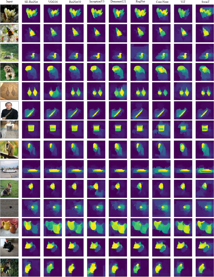
To evaluate the generality of the proposed method, well-trained deep learning classifiers with multiple different backbones were employed, including VGG16 simonyan2014very, ResNet50 he2016deep, SE-ResNet hu2018squeeze, InceptionV3 szegedy2016rethinking, DenseNet121 huang2017densely, RegNet-X-16GF radosavovic2020designing, ConvNext-Tiny liu2022convnet, ViT-L-16 dosovitskiy2020image and SwinT-Tiny liu2021swin. From Figure 3, we can see that the proposed PAMI method can robustly and precisely localize the object regions which are relevant to the model prediction for each input image, regardless of the classifier backbones. In contrast, for each representative baseline method, the importance maps often change over model backbones and even may not work for the Transformer backbone ViT and SwinT. This confirms that the proposed PAMI method is more stable and can be applied to interpretation of model predictions with various model backbones. Please see more results with consistent observations from the supplementary E.

4.5 Sensitivity and ablation study

In the proposed method, masking majority of the input is one necessary step to estimate the contribution of each single region or part of the input. There are multiple choices for the masking operator. When input is an image, the to-be-masked region could be replaced by constant intensity value such as 0 (i.e., becoming black) or 255 (i.e., becoming white), or by the blurred version of the input image. Figure 4 demonstrates exemplar results with different masking operators, which shows that masking by blurred region (‘Blurred’) results in better separation between the background regions and the object regions of interest at the first run, in turn leading to better importance maps with clearer boundaries between background and object regions at the second (i.e., final) run. When the majority of the input is replaced with extreme black or white pixels, the modified input image becomes further from the original class distribution in the feature space compared to the modified image with blurred region, which makes the model prediction unstable and therefore may not faithfully represent the importance of the preserved local region.

In addition, the average of multiple importance maps from multiple pre-segmentation algorithms often results in better visualization than that of using a single pre-segmentation algorithm, as demonstrated in Figure 5 (columns 2-5 vs. column 6). Figure 5 also shows that the second run (last column) can often refine the importance map from the first run (column 6). This is probably because sometimes the adopted pre-segmentation algorithms cannot well separate background regions from object regions at the first run, but the initially estimated importance map from the first run provides alternative information for pre-segmentation algorithms to well separate background regions from object regions. Note that the proposed PAMI is independent of the adopted pre-segmentation algorithms, and better pre-segmentation algorithms can be adopted to replace the current ones in the future. Please see more ablation study results with consistent observations from the supplementary F.

4.6 Extensive applications of the proposed PAMI

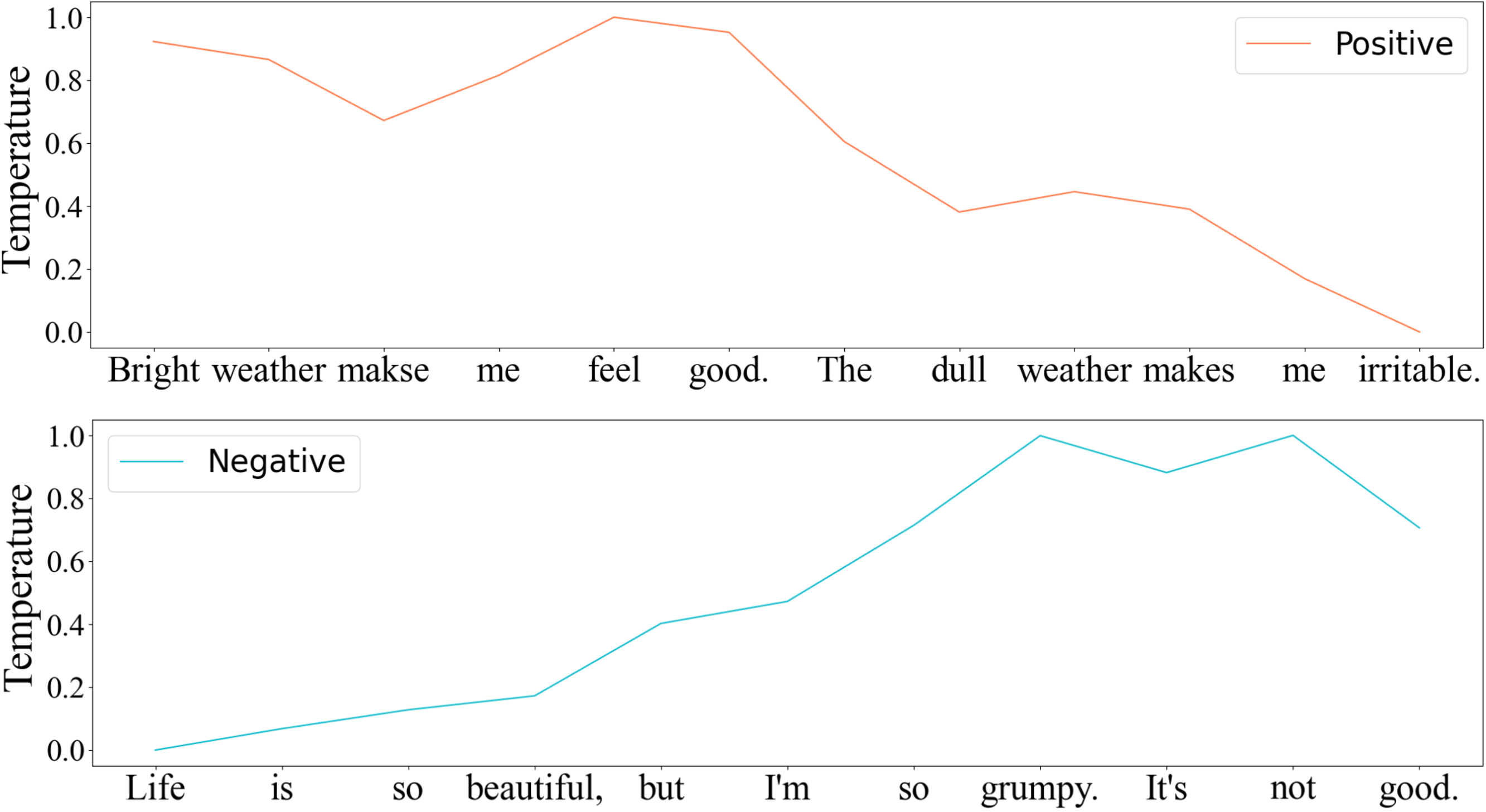
The proposed PAMI method is expected to work for multiple types of prediction tasks. For example, based on a well-trained image caption model mokady2021clipcap, the PAMI method can well localize the image regions relevant to the predicted words (e.g., ‘dog’, ‘laying’, ‘sidewalk’, ‘bicycle’) which refer to any object or behaviour in the image (Figure 6, rows 1, 3), while the representative baseline method RISE often cannot precisely localize relevant regions (Figure 6, rows 2, 4). Another example is for the sentiment analysis task, where the model tries to evaluate whether the viewpoint in an input sentence is positive or negative. With an input partition strategy (see supplementary G)) similar to the pre-segmentation for images, the proposed PAMI method can directly and correctly estimate the contribution of each word to the final model prediction (Figure 7). These results (also see more results in the supplementary G) confirm that the proposed PAMI method can work for various tasks with different input modalities.

5 Conclusion

In this study, we propose a novel visualization method PAMI for interpretation of model predictions. PAMI does not requires any model parameter details and works stably across model backbones and input formats. Compared to existing visualization approaches, PAMI can more likely and precisely find the possible local input regions which contribute to the specific model prediction to some degree. It can be used as a plug-in component and applied to multiple types of prediction tasks, which has been partly confirmed by image classification, image caption, and sentiment analysis tasks. Its utility in more tasks including various natural language processing tasks will be evaluated in future work.

References

(1) Visual explanation methods for pytorch. https://github.com/vlue-c/Visual-Explanation-Methods-PyTorch, 2020.
(2) Sebastian Bach, Alexander Binder, Grégoire Montavon, Frederick Klauschen, Klaus-Robert Müller, and Wojciech Samek. On Pixel-Wise Explanations for Non-Linear Classifier Decisions by Layer-Wise Relevance Propagation. PLoS ONE, 10(7):e0130140, 2015.
(3) Pablo Barceló, Egor V Kostylev, Mikael Monet, Jorge Pérez, Juan Reutter, and Juan-Pablo Silva. The Logical Expressiveness of Graph Neural Networks. In International Conference on Learning Representations, 2020.
(4) David Bau, Jun-Yan Zhu, Hendrik Strobelt, Agata Lapedriza, Bolei Zhou, and Antonio Torralba. Understanding the role of individual units in a deep neural network. Proceedings of the National Academy of Sciences, 117(48):30071–30078, 2020.
(5) Michael Van den Bergh, Xavier Boix, Gemma Roig, Benjamin de Capitani, and Luc Van Gool. Seeds: Superpixels extracted via energy-driven sampling. In European conference on computer vision, pages 13–26, 2012.
(6) Alexander Binder, Grégoire Montavon, Sebastian Lapuschkin, Klaus-Robert Müller, and Wojciech Samek. Layer-wise Relevance Propagation for Neural Networks with Local Renormalization Layers. In International Conference on Artificial Neural Networks, pages 63–71, 2016.
(7) G. Bradski. The OpenCV Library. Dr. Dobb’s Journal of Software Tools, 2000.
(8) Aditya Chattopadhay, Anirban Sarkar, Prantik Howlader, and Vineeth N Balasubramanian. Grad-CAM++: Generalized Gradient-Based Visual Explanations for Deep Convolutional Networks. In IEEE Winter conference on Applications of Computer Vision, pages 839–847, 2018.
(9) Hila Chefer, Shir Gur, and Lior Wolf. Transformer Interpretability Beyond Attention Visualization. In Proceedings of the IEEE Conference on Computer Vision and Pattern Recognition, pages 782–791, 2021.
(10) Sihong Chen, Kai Ma, and Yefeng Zheng. Med3D: Transfer Learning for 3D Medical Image Analysis. arXiv preprint arXiv:1904.00625, 2019.
(11) Marina Danilevsky, Kun Qian, Ranit Aharonov, Yannis Katsis, Ban Kawas, and Prithviraj Sen. A Survey of the State of Explainable AI for Natural Language Processing. In Proceedings of the 1st Conference of the Asia-Pacific Chapter of the Association for Computational Linguistics and the 10th International Joint Conference on Natural Language Processing, pages 447–459, 2020.
(12) Nima Dehmamy, Albert-László Barabási, and Rose Yu. Understanding the Representation Power of Graph Neural Networks in Learning Graph Topology. Advances in Neural Information Processing Systems, 32, 2019.
(13) Robert Desimone, John Duncan, et al. Neural mechanisms of selective visual attention. Annual Review of Neuroscience, 18(1):193–222, 1995.
(14) Alexey Dosovitskiy, Lucas Beyer, Alexander Kolesnikov, Dirk Weissenborn, Xiaohua Zhai, Thomas Unterthiner, Mostafa Dehghani, Matthias Minderer, Georg Heigold, Sylvain Gelly, et al. An Image is Worth 16x16 Words: Transformers for Image Recognition at Scale. In International Conference on Learning Representations, 2020.
(15) Andrew Elliott, Stephen Law, and Chris Russell. Explaining Classifiers using Adversarial Perturbations on the Perceptual Ball. In Proceedings of the IEEE Conference on Computer Vision and Pattern Recognition, pages 10693–10702, 2021.
(16) Dumitru Erhan, Yoshua Bengio, Aaron Courville, and Pascal Vincent. Visualizing Higher-Layer Features of a Deep Network. University of Montreal, 1341(3):1–13, 2009.
(17) Mark Everingham. The PASCAL Visual Object Classes Challenge 2007. http://www.pascal-network.org/challenges/VOC/voc2007/workshop/index.html.
(18) M. Everingham, L. Van Gool, C. K. I. Williams, J. Winn, and A. Zisserman. The PASCAL Visual Object Classes Challenge 2007 Results. http://www.pascal-network.org/challenges/VOC/voc2007/workshop/index.html.
(19) Pedro F Felzenszwalb and Daniel P Huttenlocher. Efficient Graph-Based Image Segmentation. International Journal of Computer Vision, 59(2):167–181, 2004.
(20) François-Guillaume Fernandez. Torchcam: class activation explorer. https://github.com/frgfm/torch-cam, March 2020.
(21) Ruth Fong, Mandela Patrick, and Andrea Vedaldi. Torchray. https://github.com/facebookresearch/TorchRay, 2019.
(22) Ruth C Fong and Andrea Vedaldi. Interpretable Explanations of Black Boxes by Meaningful Perturbation. In Proceedings of the IEEE International Conference on Computer Vision, pages 3429–3437, 2017.
(23) Alec Go, Richa Bhayani, and Lei Huang. Twitter sentiment classification using distant supervision. http://help.sentiment140.com/home, 2009.
(24) Jindong Gu, Yinchong Yang, and Volker Tresp. Understanding Individual Decisions of CNNs via Contrastive Backpropagation. In Asian Conference on Computer Vision, pages 119–134, 2018.
(25) Kaiming He, Xiangyu Zhang, Shaoqing Ren, and Jian Sun. Deep Residual Learning for Image Recognition. In Proceedings of the IEEE Conference on Computer Vision and Pattern Recognition, pages 770–778, 2016.
(26) Ran He, Xiang Wu, Zhenan Sun, and Tieniu Tan. Wasserstein CNN: Learning Invariant Features for NIR-VIS Face Recognition. IEEE Transactions on Pattern Analysis and Machine intelligence, 41(7):1761–1773, 2018.
(27) Jie Hu, Li Shen, and Gang Sun. Squeeze-and-Excitation Networks. In Proceedings of the IEEE Conference on Computer Vision and Pattern Recognition, pages 7132–7141, 2018.
(28) Gao Huang, Zhuang Liu, Laurens Van Der Maaten, and Kilian Q Weinberger. Densely Connected Convolutional Networks. In Proceedings of the IEEE Conference on Computer Vision and Pattern Recognition, pages 4700–4708, 2017.
(29) Laurent Itti and Christof Koch. Computational modelling of visual attention. Nature Reviews Neuroscience, 2(3):194–203, 2001.
(30) Brian Kenji Iwana, Ryohei Kuroki, and Seiichi Uchida. Explaining Convolutional Neural Networks using Softmax Gradient Layer-wise Relevance Propagation. In Proceedings of the IEEE International Conference on Computer Vision Workshop, pages 4176–4185, 2019.
(31) Peng-Tao Jiang, Chang-Bin Zhang, Qibin Hou, Ming-Ming Cheng, and Yunchao Wei. LayerCAM: Exploring Hierarchical Class Activation Maps for Localization. IEEE Transactions on Image Processing, 30:5875–5888, 2021.
(32) Been Kim, Martin Wattenberg, Justin Gilmer, Carrie Cai, James Wexler, Fernanda Viegas, et al. Interpretability Beyond Feature Attribution: Quantitative Testing with Concept Activation Vectors (TCAV). In International Conference on Machine Learning, pages 2668–2677, 2018.
(33) Yonghyun Kim, Wonpyo Park, Myung-Cheol Roh, and Jongju Shin. GroupFace: Learning Latent Groups and Constructing Group-based Representations for Face Recognition. In Proceedings of the IEEE Conference on Computer Vision and Pattern Recognition, pages 5621–5630, 2020.
(34) Pieter-Jan Kindermans, Kristof T Schütt, Maximilian Alber, Klaus-Robert Müller, Dumitru Erhan, Been Kim, and Sven Dähne. Learning how to explain neural networks: PatternNet and PatternAttribution. In International Conference on Learning Representations, 2018.
(35) Narine Kokhlikyan, Vivek Miglani, Miguel Martin, Edward Wang, Bilal Alsallakh, Jonathan Reynolds, Alexander Melnikov, Natalia Kliushkina, Carlos Araya, Siqi Yan, et al. Captum: A unified and generic model interpretability library for pytorch. arXiv preprint arXiv:2009.07896, 2020.
(36) Ruiwen Li, Zheda Mai, Chiheb Trabelsi, Zhibo Zhang, Jongseong Jang, and Scott Sanner. TransCAM: Transformer Attention-based CAM Refinement for Weakly Supervised Semantic Segmentation. arXiv preprint arXiv:2203.07239, 2022.
(37) Shaohua Li, Xiuchao Sui, Xiangde Luo, Xinxing Xu, Yong Liu, and Rick Siow Mong Goh. Medical Image Segmentation using Squeeze-and-Expansion Transformers. In International Joint Conferences on Artificial Intelligence, 2021.
(38) Xiaoxiao Li, Nicha C Dvornek, Yuan Zhou, Juntang Zhuang, Pamela Ventola, and James S Duncan. Graph Neural Network for Interpreting Task-fMRI Biomarkers. In International Conference on Medical Image Computing and Computer-Assisted Intervention, pages 485–493, 2019.
(39) Dohun Lim, Hyeonseok Lee, and Sungchan Kim. Building Reliable Explanations of Unreliable Neural Networks: Locally Smoothing Perspective of Model Interpretation. In Proceedings of the IEEE Conference on Computer Vision and Pattern Recognition, pages 6468–6477, 2021.
(40) Tsung-Yi Lin, Michael Maire, Serge Belongie, James Hays, Pietro Perona, Deva Ramanan, Piotr Dollár, and C Lawrence Zitnick. Microsoft COCO: Common Objects in Context. In European Conference on Computer Vision, pages 740–755, 2014.
(41) Sun-Ao Liu, Hongtao Xie, Hai Xu, Yongdong Zhang, and Qi Tian. Partial Class Activation Attention for Semantic Segmentation. In Proceedings of the IEEE Conference on Computer Vision and Pattern Recognition, pages 16836–16845, 2022.
(42) Ze Liu, Yutong Lin, Yue Cao, Han Hu, Yixuan Wei, Zheng Zhang, Stephen Lin, and Baining Guo. Swin Transformer: Hierarchical Vision Transformer using Shifted Windows. In Proceedings of the IEEE International Conference on Computer Vision, pages 10012–10022, 2021.
(43) Zhuang Liu, Hanzi Mao, Chao-Yuan Wu, Christoph Feichtenhofer, Trevor Darrell, and Saining Xie. A ConvNet for the 2020s. In Proceedings of the IEEE Conference on Computer Vision and Pattern Recognition, pages 11976–11986, 2022.
(44) Wenjie Luo, Yujia Li, Raquel Urtasun, and Richard Zemel. Understanding the Effective Receptive Field in Deep Convolutional Neural Networks. Advances in Neural Information Processing Systems, 29, 2016.
(45) Aravindh Mahendran and Andrea Vedaldi. Understanding Deep Image Representations by Inverting Them. In Proceedings of the IEEE Conference on Computer Vision and Pattern Recognition, pages 5188–5196, 2015.
(46) Fernand Meyer. Color Image Segmentation. In International Conference on Image Processing and its Applications, pages 303–306, 1992.
(47) Ron Mokady, Amir Hertz, and Amit H Bermano. ClipCap: CLIP Prefix for Image Captioning. arXiv preprint arXiv:2111.09734, 2021.
(48) Grégoire Montavon, Sebastian Lapuschkin, Alexander Binder, Wojciech Samek, and Klaus-Robert Müller. Explaining nonlinear classification decisions with deep Taylor decomposition. Pattern Recognition, 65:211–222, 2017.
(49) Meike Nauta, Ron van Bree, and Christin Seifert. Neural Prototype Trees for Interpretable Fine-grained Image Recognition. In Proceedings of the IEEE Conference on Computer Vision and Pattern Recognition, pages 14933–14943, 2021.
(50) Abraham Montoya Obeso, Jenny Benois-Pineau, Mireya Saraí García Vázquez, and Alejandro Álvaro Ramírez Acosta. Visual vs internal attention mechanisms in deep neural networks for image classification and object detection. Pattern Recognition, 123:108411, 2022.
(51) Utku Ozbulak. Pytorch cnn visualizations. https://github.com/utkuozbulak/pytorch-cnn-visualizations, 2019.
(52) Adam Paszke, Sam Gross, Francisco Massa, Adam Lerer, James Bradbury, Gregory Chanan, Trevor Killeen, Zeming Lin, Natalia Gimelshein, Luca Antiga, Alban Desmaison, Andreas Kopf, Edward Yang, Zachary DeVito, Martin Raison, Alykhan Tejani, Sasank Chilamkurthy, Benoit Steiner, Lu Fang, Junjie Bai, and Soumith Chintala. PyTorch: An Imperative Style, High-Performance Deep Learning Library. In Advances in Neural Information Processing Systems, pages 8024–8035, 2019.
(53) Steven E Petersen and Michael I Posner. The Attention System of the Human Brain: 20 Years After. Annual Review of Neuroscience, 35:73, 2012.
(54) Vitali Petsiuk, Abir Das, and Kate Saenko. RISE: Randomized Input Sampling for Explanation of Black-box Models. In Proceedings of the British Machine Vision Conference, 2018.
(55) Phillip E Pope, Soheil Kolouri, Mohammad Rostami, Charles E Martin, and Heiko Hoffmann. Explainability Methods for Graph Convolutional Neural Networks. In Proceedings of the IEEE Conference on Computer Vision and Pattern Recognition, pages 10772–10781, 2019.
(56) Ilija Radosavovic, Raj Prateek Kosaraju, Ross Girshick, Kaiming He, and Piotr Dollár. Designing Network Design Spaces. In Proceedings of the IEEE Conference on Computer Vision and Pattern Recognition, pages 10428–10436, 2020.
(57) Xiaofeng Ren and Jitendra Malik. Learning a Classification Model for Segmentation. In Proceedings of the IEEE International Conference on Computer Vision, pages 10–10, 2003.
(58) Marco Tulio Ribeiro, Sameer Singh, and Carlos Guestrin. “Why Should I Trust You?”: Explaining the Predictions of Any Classifier. In Proceedings of the ACM SIGKDD International Conference on Knowledge Discovery and Data Mining, pages 1135–1144, 2016.
(59) Olga Russakovsky, Jia Deng, Hao Su, Jonathan Krause, Sanjeev Satheesh, Sean Ma, Zhiheng Huang, Andrej Karpathy, Aditya Khosla, Michael Bernstein, Alexander C. Berg, and Li Fei-Fei. ImageNet Large Scale Visual Recognition Challenge. International Journal of Computer Vision, 115(3):211–252, 2015.
(60) Dawid Rymarczyk, Łukasz Struski, Jacek Tabor, and Bartosz Zieliński. ProtoPShare: Prototypical Parts Sharing for Similarity Discovery in Interpretable Image Classification. In Proceedings of the ACM SIGKDD International Conference on Knowledge Discovery and Data Mining, pages 1420–1430, 2021.
(61) Edward Sanderson and Bogdan J Matuszewski. FCN-Transformer Feature Fusion for Polyp Segmentation. In Annual Conference on Medical Image Understanding and Analysis, pages 892–907, 2022.
(62) Ramprasaath R Selvaraju, Michael Cogswell, Abhishek Das, Ramakrishna Vedantam, Devi Parikh, and Dhruv Batra. Grad-CAM: Visual Explanations from Deep Networks via Gradient-based Localization. In Proceedings of the IEEE International Conference on Computer Vision, pages 618–626, 2017.
(63) K Simonyan, A Vedaldi, and A Zisserman. Deep inside convolutional networks: visualising image classification models and saliency maps. In International Conference on Learning Representations, 2014.
(64) Karen Simonyan and Andrew Zisserman. Very Deep Convolutional Networks for Large-Scale Image Recognition. In International Conference on Learning Representations, 2015.
(65) Daniel Smilkov, Nikhil Thorat, Been Kim, Fernanda Viégas, and Martin Wattenberg. SmoothGrad: removing noise by adding noise. arXiv preprint arXiv:1706.03825, 2017.
(66) J Springenberg, Alexey Dosovitskiy, Thomas Brox, and M Riedmiller. Striving for Simplicity: The All Convolutional Net. In International Conference on Learning Representations Workshop, 2015.
(67) Suraj Srinivas and François Fleuret. Full-Gradient Representation for Neural Network Visualization. Advances in Neural Information Processing Systems, 32, 2019.
(68) Mukund Sundararajan, Ankur Taly, and Qiqi Yan. Axiomatic Attribution for Deep Networks. In International Conference on Machine Learning, pages 3319–3328, 2017.
(69) Christian Szegedy, Vincent Vanhoucke, Sergey Ioffe, Jon Shlens, and Zbigniew Wojna. Rethinking the Inception Architecture for Computer Vision. In Proceedings of the IEEE Conference on Computer Vision and Pattern Recognition, pages 2818–2826, 2016.
(70) Sho Takase and Shun Kiyono. Rethinking Perturbations in Encoder-Decoders for Fast Training. In Conference of the North American Chapter of the Association for Computational Linguistics, pages 5767–5780, 2021.
(71) Stéfan van der Walt, Johannes L. Schönberger, Juan Nunez-Iglesias, François Boulogne, Joshua D. Warner, Neil Yager, Emmanuelle Gouillart, Tony Yu, and the scikit-image contributors. scikit-image: image processing in Python. PeerJ, 2:e453, 6 2014.
(72) Eric Wallace, Matt Gardner, and Sameer Singh. Interpreting Predictions of NLP models. In Proceedings of the Conference on Empirical Methods in Natural Language Processing: Tutorial Abstracts, pages 20–23, 2020.
(73) Haofan Wang, Zifan Wang, Mengnan Du, Fan Yang, Zijian Zhang, Sirui Ding, Piotr Mardziel, and Xia Hu. Score-CAM: Score-Weighted Visual Explanations for Convolutional Neural Networks. In Proceedings of the IEEE Conference on Computer Vision and Pattern Recognition Workshop, pages 24–25, 2020.
(74) Thomas Wolf, Lysandre Debut, Victor Sanh, Julien Chaumond, Clement Delangue, Anthony Moi, Pierric Cistac, Tim Rault, Rémi Louf, Morgan Funtowicz, et al. Transformers: State-of-the-Art Natural Language Processing. In Proceedings of the Conference on Empirical Methods in Natural Language Processing: system demonstrations, pages 38–45, 2020.
(75) Lijun Wu, Juntao Li, Yue Wang, Qi Meng, Tao Qin, Wei Chen, Min Zhang, Tie-Yan Liu, et al. R-Drop: Regularized Dropout for Neural Networks. Advances in Neural Information Processing Systems, 34:10890–10905, 2021.
(76) Haoran Xu, Benjamin Van Durme, and Kenton Murray. BERT, mBERT, or BiBERT? A Study on Contextualized Embeddings for Neural Machine Translation. In Proceedings of the Conference on Empirical Methods in Natural Language Processing, pages 6663–6675, 2021.
(77) Mengjia Yan, Mengao Zhao, Zining Xu, Qian Zhang, Guoli Wang, and Zhizhong Su. VarGFaceNet: An Efficient Variable Group Convolutional Neural Network for Lightweight Face Recognition. In International Conference on Computer Vision Workshop, 2019.
(78) Jason Yosinski, Jeff Clune, Anh Nguyen, Thomas Fuchs, and Hod Lipson. Understanding Neural Networks Through Deep Visualization. In International Conference on Machine Learning Workshop, 2015.
(79) Matthew D Zeiler and Rob Fergus. Visualizing and Understanding Convolutional Networks. In European Conference on Computer Vision, pages 818–833, 2014.
(80) Jianming Zhang, Sarah Adel Bargal, Zhe Lin, Jonathan Brandt, Xiaohui Shen, and Stan Sclaroff. Top-Down Neural Attention by Excitation Backprop. International Journal of Computer Vision, 126(10):1084–1102, 2018.
(81) Bolei Zhou, Aditya Khosla, Àgata Lapedriza, Aude Oliva, and Antonio Torralba. Object Detectors Emerge in Deep Scene CNNs. In International Conference on Learning Representations, 2015.
(82) Bolei Zhou, Aditya Khosla, Agata Lapedriza, Aude Oliva, and Antonio Torralba. Learning Deep Features for Discriminative Localization. In Proceedings of the IEEE Conference on Computer Vision and Pattern Recognition, pages 2921–2929, 2016.
(83) Luisa M Zintgraf, Taco S Cohen, Tameem Adel, and Max Welling. Visualizing Deep Neural Network Decisions: Prediction Difference Analysis. In International Conference on Learning Representations, 2017.

Appendix A Hyper-parameters for pre-segmentation

The hyper-parameters of the four pre-segmentation algorithms used in both the first and the second run are summarized in table 3. The hyper-parameter names used in the methods correspond to those in the skimage and cv2 packages.

Table 3: Hyper-parameter configuration for each segmentation algorithm.

Method	Hyper-parameter
felzenszwalb felzenszwalb2004efficient	scale=250, 200, 150, 100, 70, 50 sigma=0.8 min_size=784
SLIC ren2003learning	n_segments=10, 20, 30, 40, 50, 60, 70, 80 compactness=20
SEEDS bergh2012seeds	num_superpixels=10, 20,30 num_levels=5 n_iter=10
watershed meyer1992color	markers=10, 20, 30 compactness=0.0001

Appendix B Hyper-parameters in baseline methods

Details of each baseline method and reference source code were provided in Table 4. For gradient-based methods, following the related work simonyan2014deep, the maximum importance value among the three channels at each spatial position was used as the final importance value for the spatial position in the importance map. For LRP montavon2017explaining,the values from three channels were averaged as the final result for each spatial position.

Table 4: Hyper-parameter configuration for each baseline method.

Method	Hyper-parameter	Code Source
GradCAM felzenszwalb2004efficient	The last layer of feature extractor	PyTorch CNN Visualizationsuozbulak_pytorch_vis_2022
ScoreCAM wang2020score	The last layer of feature extractor	TorchCamtorcham2020
Occlusion zeiler2014visualizing	strides=6, shapes=(3, 40, 40)	Captum kokhlikyan2020captum
RISE petsiuk2018rise	num_mask=4000, cell_size=7 probability=0.5	TorchVex torchvex
MASK fong2017interpretable	TV_beta=3, lr=0.1, max_iterations=500 l1_coeff=0.01, tv_coeff=0.2	TorchVex torchvex
FullGrad bergh2012seeds	-	original implementationsrinivas2019full

Appendix C More qualitative evaluation

C.1 More results on ImageNet-2012

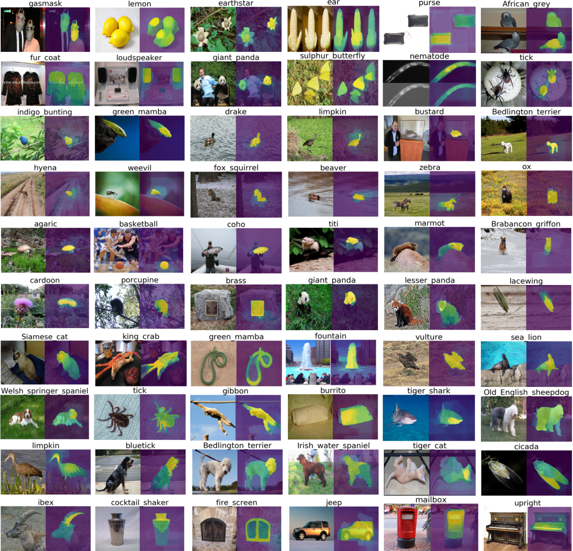
More qualitative evaluation of the proposed PAMI method on the ImageNet-2012 dataset ILSVRC15 can be seen in Figure 8, supporting the effectiveness of the method.

C.2 More results on Pascal VOC 2007

The effectiveness of the proposed PAMI method was also validated on the Pascal VOC 2007 dataset everingham2009pascal, as shown in Figure 9.

C.3 More results on COCO 2014

The effectiveness of the proposed PAMI method was also validated on the COCO 2014 dataset lin2014microsoft, as shown in Figure 10.

Appendix D Details of quantitative evaluation

For the pointing game, the process provided by TorchRay torchray was followed. On the Pascal VOC and the COCO datasets, the evaluation code provided by TorchRay was directly used, and on the ImageNet dataset, the same process was performed by marking points that fall within the bounding box of the object as hits and the rest as misses. For the insertion metric, a Gaussian kernel with size $49\times 49$ pixels and standard deviation $100$ was used to generate the blurred image where we gradually restore the original pixels from. The importance map for quantitative evaluation were generated with respect to the model output of the ground-truth class for each image. Two exemplar results were shown in Figure 11.

Appendix E Generality of the PAMI

More results with different model backbones were shown in Figure 12, supporting the generality of the proposed method.

Appendix F More ablation study results

F.1 Effect of different masking operators

More visualization results based on different masking operators were provided in Figure 13, which shows that the blurred version results in better results especially when image background is complex.

F.2 Effect of multiple pre-segmentation algorithms

More results in Figure 14 shows that using multiple pre-segmentations and two runs result in better visualizations.

Appendix G Extensive applications of PAMI

G.1 Image caption task

More experimental results for the image caption task on the COCO dataset can be seen in Figure 15.

G.2 Sentiment analysis task

More test sentences in Sentiment140 Sentiment140 were randomly selected for effectiveness evaluation of the proposed method in sentiment analysis tasks. The experimental results can be seen in Figure 16.